Inverse streamflow routing

www.hydrol-earth-syst-sci.net/17/4577/2013/ doi:10.5194/hess-17-4577-2013

© Author(s) 2013. CC Attribution 3.0 License.

Hydrology and

Earth System

Sciences

Inverse streamflow routing

M. Pan and E. F. Wood

Department of Civil and Environmental Engineering, Princeton University, Princeton, NJ, USA Correspondence to: M. Pan ([email protected])

Received: 14 May 2013 – Published in Hydrol. Earth Syst. Sci. Discuss.: 3 June 2013 Revised: 27 September 2013 – Accepted: 17 October 2013 – Published: 19 November 2013

Abstract. The process whereby the spatially distributed

runoff (generated through saturation/infiltration excesses, subsurface flow, etc.) travels over the hillslope and river net-work and becomes streamflow is generally referred to as “routing”. In short, routing is a runoff-to-streamflow process, and the streamflow in rivers is the response to runoff inte-grated in both time and space. Here we develop a method-ology to invert the routing process, i.e., to derive the spa-tially distributed runoff from streamflow (e.g., measured at gauge stations) by inverting an arbitrary linear routing model using fixed interval smoothing. We refer to this streamflow-to-runoff process as “inverse routing”. Inversion experiments are performed using both synthetically generated and real streamflow measurements over the Ohio River basin. Re-sults show that inverse routing can effectively reproduce the spatial field of runoff and its temporal dynamics from suf-ficiently dense gauge measurements, and the inversion per-formance can also be strongly affected by low gauge density and poor data quality.

The runoff field is the only component in the terrestrial water budget that cannot be directly measured, and all pre-vious studies used streamflow measurements in its place. Consequently, such studies are limited to scales where the spatial and temporal difference between the two can be ig-nored. Inverse routing provides a more sophisticated tool than traditional methods to bridge this gap and infer fine-scale (in both time and space) details of runoff from aggre-gated measurements. Improved handling of this final gap in terrestrial water budget analysis may potentially help us to use space-borne altimetry-based surface water measurements for cross-validating, cross-correcting, and assimilation with other space-borne water cycle observations.

1 Introduction

Runoff is a very important component in the terrestrial water budget (precipitation, evapotranspiration, runoff, and soil/snow water storage) in terms of both its magnitude and temporal variability (Hagemann and Dumenil, 1998; Pan et al., 2012). And runoff is also the only component in the ter-restrial water budget that cannot be measured directly at the time and location it occurs. When precipitation is measured by rain gauges, radars, or satellite sensors, the measured value is validated at the same time and location it rains or snows, and so is evapotranspiration by towers/satellites and soil moisture by probes/microwave sensors. But so far there seems to be no way of measuring the spatial field of runoff as it occurs. Therefore, previous studies used the stream-flow measurements in place of runoff (Sahoo et al., 2011; Sheffield et al., 2009). However, as streamflow can be mea-sured at river gauges and will be meamea-sured at large scales by space-borne altimetry sensors through Manning’s equation (Alsdorf and Lettenmaier, 2003), for example, the planned Surface Water and Ocean Topography (SWOT) mission (Als-dorf et al., 2011), it is not fully equivalent to runoff. So all such studies are limited to the situations/scales where the temporal and spatial difference between the two can be ei-ther ignored or somehow accounted for. For example, the river travel time may be ignored at long-term timescales. Hy-drologically, streamflow differs from runoff by one process called “routing”.

the streamflow is the response to the runoff field integrated in both time and space. Routing essentially provides a runoff-to-streamflow conversion, and it is a quite well studied pro-cess in hydrology. Routing models have been developed to parameterize this runoff-to-streamflow process and predict the streamflow at desired gauging locations given rainfall or runoff inputs (Brutsaert, 1994; Lohmann et al., 1998).

Now the question for our study is how to bridge the gap between streamflow and runoff in both time and space, i.e. to derive the spatial fields of runoff from streamflow measure-ments at gauging points, such that our water budget analysis or any related studies are no longer limited by the gap be-tween the two. Obviously, this requires us to invert the rout-ing process and invent a way to realize the streamflow-to-runoff conversion. We refer to such a streamflow-to-streamflow-to-runoff process as “inverse routing”. Note that solving inverse prob-lems is nothing new in hydrology. For example, inverse problems are frequently studied in groundwater hydrology for parameter estimation purposes (McLaughlin and Town-ley, 1996). While the general methods for solving inverse problems are no different from any other optimal estima-tion problems like data assimilaestima-tion (McLaughlin, 2002; Re-ichle, 2008), different problems may require very differ-ent methodological considerations. For example, parameter-estimation-related inverse problems usually solve for static (time-invariant) unknowns. Thus complicated and computa-tionally intensive methods may be used to invert subtly be-haved nonlinear models with non-Gaussian errors. The in-verse routing problem needs to solve for dynamic fields of runoff repeatedly in time, and thus it requires a higher com-putational efficiency. Also, the streamflow values are always correlated in time as a result of the time integration nature of the routing process, and that implies the unknown runoff fields across multiple time steps need to be solved together, which dramatically increases the size of the estimation prob-lem (number of simultaneous unknowns).

For these above reasons, we look for a linear routing model to invert such that the most efficient methods for linear sys-tems like Kalman filters/smoothers (Anderson and Moore, 1979; Kalman, 1960) can be applied. Also, inverse routing is not the only way to estimate runoff – hydrological models infer it from rainfall and other inputs, and the basin-specific discharge has always been calculated from gauge measure-ments and water balance relationship between gauge basins and their contributing sub-basins (though the fine-scale vari-ability below sub-basins is ignored). So the potential contri-bution from inverse routing should also be evaluated in terms of its “added value” to the traditional methods.

In Sect. 2, we will first introduce the routing model to use and show how to invert it using a special type of data as-similation technique called fixed interval smoothing. Then in Sect. 3 an inverse routing experiment will be performed using synthetically generated runoff/streamflow data where the inversion errors and related performance issues can be investigated against the synthetic truth. Later in Sect. 3 an

inverse routing experiment will be performed using real river gauge measurements from the United States Geological Sur-vey (USGS) to evaluate the inversion performance in real world applications. And finally the various limitations of in-verse routing will be studied in Sect. 4.

2 Methodology

2.1 A linear routing model

Here we choose the University of Washington (UW) routing model (Lohmann et al., 1996, 1998), which is a relatively simple linear routing model developed for coupling with land surface models (LSMs), and it has been calibrated, imple-mented and validated in many large-scale streamflow studies (Mitchell et al., 2004; Nijssen et al., 1997). The inputs to the UW routing model are runoff fields defined on a rectangular computing grid – the format used by most LSMs. The UW model routes the runoff water in two stages: first the runoff water drains from within the grid pixel (over the hillslope) to a conceptual “outlet” of the pixel following a known unit hy-drograph function (UHF)u(t ), and the pixel outflowo(t )is the convolution between the UHFu(t )and pixel runoffr(t ):

o(t )=

t

Z

0

r(t−τ )u(τ )dτ . (1)

Then the water travels in channels between pixels following the 1-D diffusive wave equation:

∂q

∂t =D

∂2q

∂x2−C

∂q

∂x. (2)

Hereq=q(x, t )is the streamflow generated by the pixel

out-flowo(t )at distancex downstream from the pixel.CandD

are referred to as channel wave velocity and diffusivity pa-rameters following our upstream literature (Lohmann et al., 1996, 1998). Note that a more precise name forC is in fact the wave celerity (Beven, 1979), which better distinguishes it from the fluid velocity measured in river channels. The 1-D diffusive wave equation is a standard advection–diffusion equation for transport, and it is always linear as long as nei-therCnorDis a function ofq. In other words, the wave ve-locityC and diffusivityDcan change in both time (t) (e.g., from summer to winter) and space (x) (e.g., from flat areas to mountains) as long as the values can be prescribed and are independent ofq. Retention effects (e.g., lakes and reser-voirs) are not considered. The equation is solved analytically using the convolution between the impulse response function (IRF) and pixel outflow:

q(x, t )= t

Z

0

i(x, t )= x

2t √

π t Dexp

−(Ct−x) 2

4Dt

, (4)

where i(x, t ) is called the IRF. Note that mathematically UHF is identical to IRF in their functional roles, and the two convolutions can be combined because the convolution oper-ations here are associative. Define a combined IRFh(x, t )as the convolution betweenu(t )andi(x, t ):

h(x, t )= t

Z

0

u(t−τ )i(x, τ )dτ . (5)

The combined IRFh(x, t )is the “overall” hydrograph func-tion in response to a unit runoff input from one pixel. And the two-stage routing is solved at once usingh(x, t ):

q(x, t )= t

Z

0

r(t−τ )h(x, τ )dτ . (6)

At a given gauge location g, we calculate the streamflow valueQ(g, t )by integrating (summing up) the contributions from all upstream pixels (i.e., the entire sub-basin that drains tog, noted as basin(g)):

Q(g, t )= X

basin(g)

q(x, t )= X

basin(g) t

Z

0

r(t−τ )h(x, τ )dτ . (7)

Equation (7) fully defines the integration of runoff field in space and time into the streamflow at a gauge location. As the routing model always runs in discretized time steps, the integration Eq. (7) is implemented as summations:

Q(g, t )= X

basin(g)

q(x, t )= X

basin(g) t

X

τ=0

r(t−τ )h(x, τ ). (8)

The UW routing model is fully contained in Eq. (8), and, in short, the streamflow at a gauge point is nothing but the sum of runoff from all contributing pixels in all possible lag times weighted by the overall IRF. This routing model is linear and simple, though the number of runoff inputs for streamflow calculation is very large, making the inverse problem chal-lenging.

2.2 Inversion through fixed interval smoothing

In dynamic system analysis and related estimation theories, the prediction model is mostly written in a “state space” form: the observations are written as a function of input states in a vector/matrix form with some model error termεlike y=Hx+ε. Now we rewrite Eq. (8) in this form. Say we havemgauge locations andnrunoff computing pixels in the study area, and we define the streamflow observation vector y_tand runoff state vectorxt as the collection of allmgauge

measurementsQ1, Q2, . . . , Qmand runoff states in alln

pix-elsr1,r2, . . . , rnat timet:

y_t=

     Q1 Q2 .. . Qm      t

andxt=

     r1 r2 .. . rn      t . (9)

As a result of the time integration in Eq. (8), the calcula-tion ofy_t requires not onlyxt but also runoff fields at

pre-vious time stepsxt−1,xt−2, . . . ,xt−k. Physically, all the lag

times within the longest travel time to the gauges should be included (i.e., until the last bit of runoff from the farthest pixel in the basin passes the most downstream gauge). Say the maximum travel time isk+1 time steps, and the observa-tion equaobserva-tion is

y_t=H0xt+H1xt−1+ · · · +Hkxt−k+εt. (10) H0, H1, . . ., Hk are the measurement operator matrices for

different lag times and each has the sizem×n. The entries in the operator reflect how much of the runoff from one specific pixel contributes to one specific gauge at a specific lag time. All of them are calculated from the combined IRFh(x, t )

according to the downstream travel distance and lag time. Again, because of the time integration, direct inversion of Eq. (10) is impossible and incomplete because streamflow at future time steps also contains information about the runoff at current time step, and the time series of streamflow are highly correlated. This means the inverse estimation must be done for multiple time steps at once, and observation and state vectors need to be “augmented” to include multiple time steps. Writing Eq. (10) for alls+1 time steps in the time interval[t−s, t], we have

y_t=H0xt+H1xt−1+ · · · + Hkxt−k +εt yt−1= H0xt−1+H1xt−2+ · · · + Hkxt−k−1 +εt−1

..

. . .. . .. . .. ...

yt−s= H0xt−s+H1xt−s−1+ · · · +Hkxt−s−k+εt−s

(11) And define the time-augmented streamflow/runoff/error vec-tors as

y0_t=

     y_t y_t−1

.. .

y_t−s



   

, x0_t=

     xt

xt−1

.. .

xt−s



   

,andε0_t=

     εt

εt−1

.. .

εt−s

     , (12)

wherey0

t has the sizem(s+1)andx0t has the sizen(s+1).

In the above, the augmented observation operator matrix H0

is

H0=



      

H0 · · ·Hk . ._. . ._.

H0 · · ·Hk . ._. .._. H0



      

. (14)

H0 is mostly empty except the upper diagonal belt is filled with H0,H1, . . . ,Hk, and it has the sizem(s+1)×n(s+1).

The augmented observation equation has one extra term compared to the un-augmented one:x0_t−k multiplied by L0, which is

L0=



       0

. ._. Hk

.. .. .. H1 · · ·Hk



      

. (15)

L0has the same size as H0:m(s+1)×n(s+1). It is empty for the firstm(s+1−k)rows andn(s+1−k)columns, and the remainingmk×nk block at the lower right corner is filled with H1, H2, . . . ,Hk in the lower diagonal. The extra term L0_x0

t−kprovides the routing model the initial conditions – the

water stored in river channels contributed by runoff in thek

time steps prior to timet−s(i.e., interval[t−s−k, t−s−1]). The time interval of augmentation needs to be larger than the maximum travel time (i.e.,s+1> k+1). This is because the streamflow measured at the outlet of the basink+1 time steps later still contains information about the runoff gener-ated at the most upstream pixel of the basin at the current time step. To enable the inversion to use all possible stream-flow information from all gauges to update the most upstream pixel, there must bes+1> k+1.

Now we can apply the Kalman-type methods for the in-version. Since we always have a fewer number of gauges than runoff pixels (i.e.,m < n), the inverse problem is under-constrained. Therefore, an initial guess of runoff fields, noted asxˆ0_t, is usually needed to represent the prior information we have on this variable. This initial guess could just be a uni-form field of long-term mean runoff (or simply zeros), which is referred to as the “null” initial guess, or LSM estimates forced with some baseline rainfall (better choice) if possi-ble. Note that the “null” initial guess is equivalent to having no initial guess at all. Given the initial guessxˆ0_t and stream-flow measurementsy0_t, the Kalman filter equation gives an updated estimatexˆ00_t as

ˆ

x00_t = ˆx0_t+Kt(y0t−H

0_xˆ0

t−L

0_xˆ0

t−k). (16)

And the Kalman gain Kt is calculated as Kt =PtH0T

H0PtH0T +Rt

−1

. (17)

Kt has the sizen(s+1)×m(s+1), and Pt is the error

co-variance matrix of the initial guess of runoff and has the size

n(s+1)×n(s+1). Pt can simply be a diagonal matrix of

the long-term mean runoff error variance, or with diagonal entries proportional to the squared runoff if the initial guess is not uniform. Rtis the error covariance matrix of the gauge

measurements and has the sizem(s+1)×m(s+1). Rt can

be looked up from river gauge documentations or empirically estimated from instrumentation type, flow rate, channel mor-phology, etc. However, here we want to force the updated runoff field to reproduce the streamflow observed at all the gauges exactly, i.e., to make the updated runoff fieldxˆ00_t to satisfy Eq. (13) with no errors:

y0_t=H0xˆ00_t +L0x0_t−k. (18) This exact match is achieved by treating the gauge measure-ments as error-free (i.e., Rt≡0), and Eq. (16) will push all

the streamflow errors in the initial guessy0_t−H0xˆ_t0−L0xˆ0_t−k

back to the runoff guess and effectively force Eq. (18) to be exactly satisfied. Caution is needed here that treating the gauge measurements as perfect does not mean we believe there are no errors in them. There are definitely errors, and such treatment is merely a way to force the exact reproduc-tion of streamflow, and all of the gauge errors will be carried into the inverted runoff. Also, such a setting maximizes the correction Eq. (16) can impose onto the initial runoff guess (Pan and Wood, 2010). This is a same measure as taken by the constrained data assimilation procedures (Pan and Wood, 2006; Pan et al., 2012). Now the Kalman gain becomes

Kt=PtH0T

H0PtH0T

−1

. (19)

Note that the above update procedures are no different than a regular data assimilation when Rt is not particularly chosen.

And in fact, many studies have been devoted to the assimi-lation of streamflow or water altimetry measurements (An-dreadis et al., 2007; Biancamaria et al., 2011; Durand et al., 2008). We would like to call the runoff estimation with the particular setting of Rt≡0 as “inverse routing”, in order to

differentiate it from the general practice of streamflow assim-ilation. Also, since the inversion involves multiple time steps, the procedure is no longer a filtering operation but a smooth-ing operation or, more precisely, as+1 step fixed interval smoothing.

During the Kalman gain calculation in Eq. (19), the ma-trix H0_P

tH0T to invert has the sizem(s+1)×m(s+1). As

matrix inversion has its computational complexity grow cu-bically against matrix size, the interval sizes+1 and num-ber of gaugesmto use cannot be too large. Per discussion on the time augmentation,s+1 has to be larger thank+1. Note that even withs+1> k+1, updating the runoff in the lastk+1 time steps in the[t−s, t]smoothing interval (i.e.,

[t−k, t]) still requires streamflow information beyond time

-80 -80

-85 -85

40 40

35 35

Ohio River

Tennesse

e River USGS GaugeDrainage Area (km2 )

< 3000 3000 - 10000 10000 - 30000 30000 - 100000 > 100000

Fig. 1. The Ohio River basin (shaded area) and 75 USGS river

gauges in use.

not receive all possible streamflow information. To elimi-nate such an “edge effect” of fixed interval smoothing, the smoothing will be done interval by interval sequentially, and consecutive intervals will overlap by k+1 steps. In other words, only the firsts−k steps in thes+1 smoothing in-terval are usable, and the lastk+1 steps will be re-updated in the next smoothing interval.

3 Inverse routing experiments

3.1 Study area and general setups

We choose the Ohio River basin in United States for the inversion experiments. Figure 1 shows the definition of the Ohio River basin, which also includes the Tennessee River in the south and covers an area of 490 600 km2. Rivers in the area are very well monitored by the United States Geologi-cal Survey (USGS), and we select 75 USGS river gauge sta-tions out of all available ones (i.e.,m=75). Gauge stations that are too close to each other were selectively removed to reduce redundancy. The computing grid for the UW rout-ing model is set up at 0.125◦and the flow network on this grid is derived from 30 arcsec digital elevation model (DEM) data, as shown in Fig. 2. The computing grid consists of 3681 0.125◦pixels (i.e.,n=3681). All routing model parameters are identical to those used in the National Land Data Assim-ilation (NLDAS) project (Lohmann et al., 2004, Mitchell et al., 2004) over the same area, where the same routing model has been calibrated and validated against USGS-observed streamflow. The channel wave velocity C=1.4 m s−1 and diffusivityD=0 m2s−1are constant all over the basin. The time step of the routing model is 1 day, and because the 0.125◦pixel is small enough for any runoff to flow out of the pixel within 1 day, the outflow UHFu(t )=1 whent=1 and

u(t )=0 whent >1. The resulted runoff water travel time to

Travel Time (days)

0 5 10 15

Fig. 2. Flow paths over the 0.125◦grid and runoff travel time to the basin outlet.

the basin outlet can be found in Fig. 2, and the maximum travel time is 16 days (i.e.,k+1=16). The study period is the entire year (365 days) of 2009.

Two types of inversion experiments will be performed where the streamflow (y0_t in Eq. 16) to be inverted is gen-erated differently:

1. Inversion experiment with synthetically generated streamflow, or in short synthetic experiment.

In this experiment, we assume the “true” values of runoff and streamflow are known, and the synthetically “true” streamflow values will be inverted (i.e., be assimilated into the initial guess of runoff) (xˆ0_t in Eq. 16). Then errors in the inverted runoff (xˆ00_t in Eq. 16), and initial guess as well, will be calculated against the synthetically “true” runoff. To do this, the synthetically “true” runoff fields will first be cre-ated by running the variable infiltration capacity (VIC) LSM (Liang et al., 1994, 1996) forced with the 0.125◦NLDAS me-teorological data set (Cosgrove et al., 2003). NLDAS rainfall combines hourly WSR-88D radar analyses and daily gauge reports (∼13 000 per day) and is considered the best avail-able surface forcing over United States. Given the NLDAS-derived “true” runoff, the synthetically “true” streamflow is created using the UW routing model. Then with an initial guess of runoff, the inversion is performed, and the errors are calculated against the NLDAS-derived synthetic truth. The benefit of a synthetic experiment is that the performance of the inversion method can be well evaluated using the syn-thetic truth. Also, as the model-derived streamflow is assim-ilated, the complications caused by errors/biases in the rout-ing model are avoided.

2. Inversion experiment with real streamflow measure-ments, or in short real experiment.

50 100 150 200 250 300 350 0

5000 10000

a) USGS 03216600, 160511 km2 USGS Measurements

Synthetic TruthQ(NLDAS-derived)

50 100 150 200 250 300 350

0 2000 4000

b) USGS 03086000, 50483 km2

Streamflow (m

3/s)

50 100 150 200 250 300 350

0 1000 2000

c) USGS 03290500, 15999 km2

50 100 150 200 250 300 350

0 200 400 600

d) USGS 03379500, 2928 km2

Day in 2009

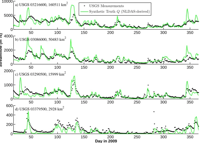
Fig. 3. Streamflow predictions from the routing model using the synthetically “true” NLDAS rainfall (green line) versus USGS measurements

(black dots) over four gauge stations. The USGS gauge station number and drainage area are noted in the panel title.

and actual measurements from USGS at four gauge stations with drainage area ranging from 160 511 km2 (Fig. 3a) to 2928 km2(Fig. 3d). As the routing model reasonably repro-duces the gauge measurements, both timing and magnitude errors can be seen, especially for larger sub-basins. Such er-rors will corrupt the performance of inverse routing, and the performance assessment from the synthetic experiment will be discounted when real gauge measurements are used. The purpose of the real experiment is to find out how much the performance degradation is and how that affects the useful-ness of inverse routing. Besides routing model errors, LSM and its parameters/input data also have errors, and that makes the NLDAS-derived runoff not really a “truth”. In the real experiment, errors will still be calculated against NLDAS-derived runoff, even though the latter is no longer a “truth”.

In both the synthetic and real experiments, the smoothing interval for the inversion is 70 days (i.e., s+1=70). The routing model spins up during the first 16 days of 2009 to provide initial conditions for later routing, and the inversion starts on day 17 of 2009.

3.2 Experiment with synthetically generated

streamflow

Here we further consider two different ways of creating the initial guess of runoff (xˆ0_t in Eq. 16). The first is the “null” initial guess mentioned in the methodology section. This is to assume we have no alternative source of runoff informa-tion at all, and the initial guess is simply a uniform field of constant value for all the time steps. Here we set it to a long-term mean value of 1.474 mm day−1. Figure 4 presents the

inversion results for day 75 of 2009 using the null initial guess of runoff. The inverted runoff field shown in Fig. 4c shows a very similar spatial pattern to the NLDAS-derived synthetic truth in Fig. 4b. The two rainfall/runoff belts in the synthetic truth, one of which goes through the north-eastern and northwestern tips of the basin and the other in the southern half (mostly over Tennessee River), have been well recovered in the inverted runoff. Note that the initial guess has no spatial variability at all (Fig. 4a). The empty area between the two belts is also fairly well cleared in the inverted runoff. The inversion increment (Fig. 4d), i.e., the difference between the inverted and the initial guess or

ˆ

x00_t− ˆx0_t=Kt(y0t−H0xˆ

0

t−L0xˆ

0

t−k)as in Eq. (16), shows where

a) Initial Guess (Null, 1.474 mm/day) b) Synthetic Truth (NLDAS−derived)

mm/day 0 0.5 1 1.5 2 2.5

c) Inverted d) Inversion Increment

mm/day −2 −1 0 1 2

Fig. 4. Runoff estimates for day 75 of 2009 from the synthetic

experiment using the null initial guess of runoff (constant field of

1.474 mm day−1): (a) initial guess, (b) synthetic truth, (c) inverted

fields, and (d) the difference between the inverted and initial guess (i.e., inversion increment during the smoothing update).

than others (e.g., day 177). In other words, the inversion also recovers a reasonable timing of the runoff. Figure 5 (bot-tom row) also shows the 7-day mean antecedent precipita-tion for those 4 days, and most of the spatial patterns in the antecedent precipitation are reasonably reflected in the in-verted runoff fields. The inversion problem from streamflow to runoff is extremely under-constrained here (m=75 ver-susn=3681), and such results suggest the inversion method has a very strong capability. The ability to work under null initial guess (i.e., no initial guess at all) has a critical mean-ing for our study. This is because in this case the streamflow measurements are the only input to the estimation problem and that means the runoff fields derived from the observed streamflow are also a purely “observationally based” quan-tity with no influence from an LSM.

Another way to create the initial guess is to use the LSM to calculate runoff from some baseline rainfall inputs that are considered always available for all locations and all times. This is supposedly a better initial guess than the null guess. It should provide a better assessment of the inverse routing than the null initial guess experiment since it is not real-istic that we know nothing about the rainfall all the time. Here we force VIC LSM with the satellite rainfall product TRMM Multi-satellite Precipitation Analysis (TMPA) ver-sion 3B42RT (Huffman et al., 2007) to obtain an initial guess of runoff. TMPA is available globally between 60◦S and 60◦N every 3 h at 0.25◦ resolution. Though much less ac-curate than the ground-based NLDAS, it relies only on satel-lites and thus is available almost everywhere. The 0.25◦data are interpolated to 0.125◦in order to force VIC simulations at 0.125◦(Pan et al., 2010). Figure 6 shows the inversion re-sults using the TMPA-derived initial guess of runoff for the

Synthetic Truth

Day 37

Inverted

Precipitation

Day 107 Day 177 Day 317

mm/day0 1 2 3

mm/day0 2 4 6 8

Fig. 5. Synthetic truth (NLDAS-derived) runoff, inverted runoff,

and 7-day antecedent precipitation (NLDAS) for another 4 days (day 37, 107, 177, and 317 of 2009) from synthetic experi-ment using the null initial guess of runoff (constant field of

1.474 mm day−1).

a) Initial Guess (TMPA−derived) b) Synthetic Truth (NLDAS−derived)

mm/day 0 0.5 1 1.5 2 2.5

c) Inverted d) Inversion Increment

mm/day −2 −1 0 1 2

Fig. 6. The same runoff plots as Fig. 4 from the synthetic experiment

using the TMPA-derived runoff field as initial guess.

same day 75 of 2009 as in Fig. 4. The inverted runoff here is similar to the null guess case in Fig. 4 but with a slightly better definition of the rainfall/runoff plumes. The transition from wet to dry areas is also smoother (i.e., less gauge basin-shaped patchiness). This suggests a good initial guess that can reasonably represent the spatial and temporal dynam-ics of rainfall will help improve the quality of the inverted runoff.

50 100 150 200 250 300 350 −5

0 5

Bias (mm/day)

a) Basin Mean Bias

Time Average (Absolute Bias) = 0.553 mm/day (Initial Guess) and 0.145 mm/day (Inverted)

Initial Guess (TMPA-derived)r

Invertedr

50 100 150 200 250 300 350

0 5 10 15 20

Day in 2009

RMSE (mm/day)

b) Basin Root Mean Squared Errors

Time Average = 1.962 mm/day (Initial Guess) and 1.283 mm/day (Inverted)

Fig. 7. Time series of basin mean bias (a) and root mean squared errors (b) from the synthetic experiment using TMPA-derived runoff

as initial guess. Blue lines are for the initial guess of runoff (TMPA-derived) and red lines for the inverted runoff. All error measures are calculated against NLDAS-derived synthetic truth runoff.

50 100 150 200 250 300 350

0 5000 10000 15000

a) USGS 03216600, 160511 km2 Synthetic TruthQ(NLDAS-derived)

Initial GuessQ(TMPA-derived)

QReconstructed from Invertedr

50 100 150 200 250 300 350

0 1000 2000 3000

b) USGS 03086000, 50483 km2

Streamflow (m

3/s)

50 100 150 200 250 300 350

0 2000 4000

c) USGS 03290500, 15999 km2

50 100 150 200 250 300 350

0 500 1000

d) USGS 03379500, 2928 km2

Day in 2009

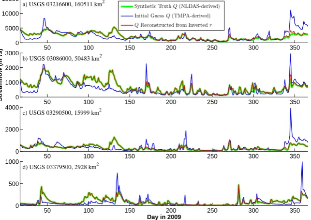
Fig. 8. Time series of streamflow estimates from the inversion experiment using TMPA-derived runoff as initial guess at four USGS gauge

stations. Thick green lines are for the synthetic truth (NLDAS-derived), blue for the initial guess (TMPA-derived), and red for the streamflow reconstructed from the inverted runoff.

0.145 mm day−1for the inverted runoff and 0.553 mm day−1 for the initial guess, and the relative bias reduction is about 74 %. However, smaller bias in the basin mean does not nec-essarily imply small errors in the pixel-to-pixel comparisons since positive and negative errors on the same map can aver-age out. Figure 7b shows the time series of basin mean root mean squared errors (RMSEs), and the inverted runoff still has a consistently lower RMSE than the initial guess but to a lesser degree. The time average of RMSE is 1.283 mm day−1 for the inverted runoff and 1.962 mm day−1 for the initial guess (about 35 % RMSE reduction).

Synthetic Truth

Day 37

Inverted

Day 107 Day 177 Day 317

mm/day0 1 2 3

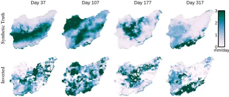
Fig. 9. Synthetic truth (NLDAS-derived) and inverted runoff fields

for 4 days (day 37, 107, 177, and 317 of 2009, same as Fig. 5) from the real experiment using TMPA-derived runoff field as initial guess and real USGS gauge measurements.

inverted runoff. Note that the streamflow time series recon-structed from the inverted runoff (red line) lies exactly on top of the synthetic truth (thick green line) nearly all the time. This verifies the fact that our setting of Rt ≡0 will force

the inverted runoff to reproduce the input streamflow exactly (Eq. 18). Perfect reproduction of input streamflow is an im-portant purpose of our inversion design, and it distinguishes the “inversion” from the streamflow data assimilation in a general sense. There are a few occasions, for example, during the few days before day 350 of 2009 at USGS gauge sta-tion 03216600 (Fig. 8a), where the inverted runoff leads to a slightly higher streamflow than the synthetic truth. This is be-cause the inversion update may, under some rare occasions, produce negative runoff values, and such negative values are reset to zero.

3.3 Experiment with real streamflow measurements

The real experiment using USGS gauge measurements is carried out only with the TMPA-derived runoff as the ini-tial guess. Some of 75 USGS gauge stations used here have missing data, but a vast majority (67 stations) of them are fairly complete for the year 2009 (available more than 95 % of the time). Figure 9 shows the inverted runoff fields ver-sus the NLDAS-derived synthetic truth (no longer treated as a “truth” here though) for the same 4 days as in Fig. 5. Here the inverted runoff fields have larger discrepancies against the NLDAS-derived values than those in the synthetic exper-iment (Fig. 5). The inverted runoff can capture some large spatial features in the NLDAS-derived map, but a lot of de-tailed spatial features differ from the NLDAS-driven syn-thetic truth. Figure 10 plots the same time series of basin mean bias and RMSE as Fig. 7. In Fig. 10a, the inverted runoff (red line) still shows a consistently lower basin mean bias than the initial guess (blue line), though not as signif-icant as in Fig. 7. The time average of the absolute bias is reduced from the 0.553 mm day−1 for the initial guess to 0.392 mm day−1 for the inverted runoff. The relative bias reduction is 29 % (compared to 74 % in the synthetic ex-periment in Fig. 7). The basin mean RMSE (Fig. 10b) for

the inverted runoff (red line) has lower peaks than the ini-tial guess (red line) but is often higher than the iniini-tial guess elsewhere. The time average of RMSE is 1.970 mm day−1, and this is even slightly higher than the TMPA-derived initial guess (1.962 mm day−1). This suggests it is more difficult to make significant improvement to the initial guess using real gauge measurements, especially when the initial guess is al-ready very reasonable. Large biases can be easily corrected, but small spatial details are much more difficult to recover.

Many factors contribute to this degraded inversion per-formance in the real experiment. Generally speaking, it is because of the routing model errors (Fig. 3). For example, model assumptions like runoff water flows in 0.125◦ digi-tized stream channels can be a reason, and model parameters (constant wave velocity/diffusivity everywhere) are far from perfect as well. Another very important reason is that many water regulation structures (dams, reservoirs, etc.) operate in this area, and the USGS-measured streamflow is not the nat-ural flow. Moreover, while the inversion treats the streamflow inputs as perfect observations, the USGS measurements are never perfect, and errors exist in both the instruments and the stage-flow regressions. Such errors are entirely carried into the inverted runoff because of this treatment. Figure 3 also shows that the NLDAS-derived streamflow compares better to the USGS measurements at gauges of smaller drainage basins (Fig. 3c, d) than large ones (Fig. 3a, b). A possible reason is that smaller basins are less affected by flow regu-lations. Unfortunately, dam/reservoir operations are mostly nonlinear (i.e., to cut flood peak or retain water for dry sea-son release), and the best way to reduce their impact is to perform streamflow naturalization (Wurbs, 2006) separately before the inversion or to avoid using gauges of heavily regu-lated large basins. Finally, NLDAS and VIC LSM have errors too, and the synthetic truth being compared is not an exact truth.

4 Limitations of inverse streamflow routing

50 100 150 200 250 300 350 −5

0 5

Bias (mm/day)

a) Basin Mean Bias

Time Average (Absolute Bias) = 0.553 mm/day (Initial Guess) and 0.392 mm/day (Inverted)

Initial Guess (TMPA-derived)r Invertedr

50 100 150 200 250 300 350

0 5 10 15 20

Day in 2009

RMSE (mm/day)

b) Basin Root Mean Squared Errors

Time Average = 1.962 mm/day (Initial Guess) and 1.970 mm/day (Inverted)

Fig. 10. Time series of basin mean bias (a) and root mean squared errors (b) from the real experiment using TMPA-derived runoff field as

initial guess and real USGS gauge measurements. All lines are plotted the same way as in Fig. 7.

0 25 50 75 0 0.2 0.4 0.6

Abs Bias (mm/day) No Error/Missing

Initial Guess a)

0 25 50 75 1 1.5 2

RMSE (mm/day)

No Error/Missing Initial Guess e)

Number of Gauges

0 50 100 0

0.2 0.4 0.6 b)

0 50 100 1

1.5 2 f)

Missing Obs (%)

0 10 20 30 0

0.2 0.4 0.6 c)

0 10 20 30 1

1.5 2 g)

Obs Error (%)

0 1 2

0 0.2 0.4 0.6 d)

0 1 2

1 1.5 2 h)

Velocity Error (m/s)

Fig. 11. Degradation of inversion performance as measured by

growing time-averaged absolute bias (upper row) and RMSE (lower row) in the inverted runoff from the synthetic experiment using TMPA-derived runoff as initial guess. The degradation test is car-ried out with respect to four sensitivity factors: fewer gauges (first column), missing gauge observations (second column), gauge ob-servation errors (log standard deviation of lognormal errors, third column), and wave velocity errors in the routing model (standard deviation of normal errors, fourth column). The absolute bias and RMSE in the inverted runoff without errors/missing data and in the initial guess are shown as solid and dashed lines.

experiments in the previous section are conducted over a heavily gauged basin with good-quality data, and those find-ings may not apply to many other places.

Now we study how the performance of inverse routing will degrade by repeating the synthetic experiment using TMPA-derived runoff as initial guess (Figs. 6 and 7) and adding er-rors and missing data to various inputs. The same two perfor-mance metrics, the time-averaged absolute bias and RMSE in the inverted runoff, are evaluated, and the degradation is tested with respect to four factors: (1) number of gauges available (from full 75 down to 4); (2) amount of missing streamflow observations, as measured by the missing per-centage (0–100 %); (3) gauge observation errors, as

mea-sured by the log standard deviation of lognormal errors (0– 30 %); and (4) wave velocity errors in the routing model, as measured by the standard deviation of normal errors (0– 2 m s−1). All the errors added are uncorrelated in time or space. Figure 11 shows how the bias and RMSE grow as more errors and missing data are added. In the case of fewer gauges and missing observations (Fig. 11a, b, e, f), both the bias and RMSE grow slowly at first, then faster, and finally approach the level of initial guess (dashed lines in Fig. 11) as the availability is reduced to zero. Note that per-formance worse than the initial guess means that the inver-sion is completely useless. Errors (lognormal) in gauge ob-servations have a large impact on the runoff RMSE (Fig. 11g) – 20 % lognormal errors can consume all the potential RMSE improvement while the bias is less affected (Fig. 11c). The wave velocity errors in the routing model also matter but to a lesser extent (Fig. 11d, h), and this parameter can usu-ally be well estimated through careful calibrations. No joint sensitivity test is carried out although multiple factors will exacerbate the performance degradation. The above findings suggest that some reasonable gauge density (e.g., more than 10 gauges per 106km2) and data quality (e.g., lower than 25 % errors) are required for the inverse routing to provide improvements to TMPA-derived runoff fields. Such require-ments may be lowered at places where TMPA performs less well. For example, TMPA is much less well calibrated in Africa than in United States because the rain gauge data there are very sparse.

5 Conclusions

The synthetic experiment shows that the inversion method is able to reproduce reasonably the spatial and temporal dynamics of the synthetically true runoff fields from point measurements of streamflow without any meaningful initial guess provided that sufficient gauge data exist. Besides the routing model and its parameters, the only input required by the inversion is streamflow. So inverse routing is always possible as long as sufficiently dense streamflow data are available. If a reasonable initial guess of runoff exists (e.g., from LSM), such an initial guess can help improve the qual-ity of the inverted runoff.

The real experiment illustrates how the inversion perfor-mance will degrade when real river gauge measurements are used. The difference between the real and synthetic stream-flow data is basically caused by the routing model errors. Such errors could be due to imperfect model design or pa-rameters, but a large part is due to the human regulation of flow – an effect unaccounted for in the routing model. In short, the inverse routing can work well only if the (forward) routing model works well, and that requires efforts in routing model calibration, streamflow naturalization, etc.

The limitations of inverse routing arise primarily from two aspects – (1) the performance of the forward routing model and its failure to account for nonlinear flow behavior like retention, and (2) gauge data availability and quality. Low gauge density and poor data quality can strongly affect the usefulness of inverse routing.

Inverse routing may be performed to infer runoff at any fine scales where the routing model is parameterized, though the quality of fine-scale information so derived is determined by the density and quality of input gauge data. Historically, runoff has not been an observationally based variable, and streamflow measurements are used in its place and such stud-ies are limited to the occasions where the mismatch between the two in time and space can be ignored. Now inverse rout-ing provides a more sophisticated tool than traditional meth-ods to resolve the scale mismatch and infer fine-scale de-tails (in both time and space) of runoff from aggregated mea-surements. Improved handling of this final gap in terrestrial water budget analysis may potentially help us to use space-borne altimetry-based surface water measurements for cross-validating and cross-correcting other space-borne water cy-cle observations. For example, given the strong tie between the rainfall and runoff, as shown in Fig. 5, runoff fields in-verted from the future SWOT mission can be used to iden-tify and correct missing or overestimated precipitation es-timates from the Global Precipitation Measurement (GPM) mission (Tapiador et al., 2012) through the water balance relationship and with the help of a hydrological model to resolve the rainfall-to-runoff process. It also makes it more convenient to assimilate the surface water measurements into other water cycle observations without worries about scale mismatch. The inverse routing is also a good tool to disag-gregate streamflow information in time and space and pro-vide more continuous and better river information for water

resources management. Without satellite altimetry measure-ments, runoff fields derived from ground river gauges can help us study the long-term terrestrial water budget at a much higher spatial and temporal resolution.

Acknowledgements. This study has greatly benefited from Colby

K. Fisher’s work on the calculation of Kalman gain. The research is supported by National Aeronautic and Space Administration (NASA) grant NNX08AN40A “Developing Consistent Earth System Data Records for the Global Terrestrial Water Cycle”.

Edited by: M. Weiler

References

Alsdorf, D. E. and Lettenmaier, D. P.: Tracking fresh water from space, Science, 301, 1491–1494, 2003.

Alsdorf, D. E., Lettenmaier, D. P., and Mognard, N. M.: Re-mote Sensing of Surface Water and Recent Developments in the SWOT Mission, in: Fall Meeting of the AGU, Session H21J-06, San Francisco, CA, 2011.

Anderson, B. D. O. and Moore, J. B.: Optimal Filtering, Prentice Hall, New York, 1–348, 1979.

Andreadis, K. M., Clark, E. A., Lettenmaier, D. P., and Als-dorf, D. E.: Prospects for river discharge and depth esti-mation through assimilation of swath-altimetry into a raster-based hydrodynamics model, Geophys. Res. Lett., 34, L10403, doi:10.1029/2007GL029721, 2007.

Beven, K.: Generalized Kinematic Routing Method, Water Resour. Res., 15, 1238–1242, 1979.

Biancamaria, S., Durand, M., Andreadis, K. M., Bates, P. D., Boone, A., Mognard, N. M., Rodriguez, E., Alsdorf, D. E., Lettenmaier, D. P., and Clark, E. A.: Assimilation of virtual wide swath al-timetry to improve Arctic river modeling, Remote Sens. Envi-ron., 115, 373–381, 2011.

Brutsaert, W.: The Unit Response of Groundwater Outflow from a Hillslope, Water Resour. Res., 30, 2759–2763, 1994.

Cosgrove, B., Lohmann, D., Mitchell, K., Houser, P., Wood, E., Schaake, J., Robock, A., Marshall, C., Sheffield, J., Duan, Q., Luo, L., Higgins, R., Pinker, R., Tarpley, J., and Meng, J.: Real-time and retrospective forcing in the North American Land Data Assimilation System (NLDAS) project, J. Geophys. Res.-Atmos., 108, 8842, doi:10.1029/2002JD003118, 2003.

Durand, M., Andreadis, K. M., Alsdorf, D. E., Lettenmaier, D. P., Moller, D., and Wilson, M.: Estimation of bathymetric depth and slope from data assimilation of swath altimetry into a hydrodynamic model, Geophys. Res. Lett., 35, L20401, doi:10.1029/2008GL034150, 2008.

Hagemann, S. and Dumenil, L.: A parametrization of the lateral waterflow for the global scale, Clim. Dynam., 14, 17–31, 1998. Huffman, G. J., Adler, R. F., Bolvin, D. T., Gu, G., Nelkin, E.

J., Bowman, K. P., Hong, Y., Stocker, E. F., and Wolff, D. B.: The TRMM multisatellite precipitation analysis (TMPA): Quasi-global, multiyear, combined-sensor precipitation estimates at fine scales, J. Hydrometeorol., 8, 38–55, 2007.

Liang, X., Lettenmaier, D. P., Wood, E. F., and Burges, S. J.: A Sim-ple Hydrologically Based Model of Land-Surface Water and En-ergy Fluxes for General-Circulation Models, J. Geophys. Res.-Atmos., 99, 14415–14428, 1994.

Liang, X., Wood, E. F. and Lettenmaier, D. P.: Surface soil moisture parameterization of the VIC-2L model: Evaluation and modifi-cation, Global Planet. Change, 13, 195–206, 1996.

Lohmann, D., Nolte-Holube, R., and Raschke, E.: A large-scale hor-izontal routing model to be coupled to land surface parametriza-tion schemes, Tellus A – Dyn. Meteorol. Oceanogr., 48, 708– 721, 1996.

Lohmann, D., Raschke, E., Nijssen, B., and Lettenmaier, D.: Re-gional scale hydrology: I. Formulation of the VIC-2L model cou-pled to a routing model, Hydrol. Sci. J., 43, 131–141, 1998. Lohmann, D., Mitchell, K., Houser, P., Wood, E., Schaake, J.,

Robock, A., Cosgrove, B., Sheffield, J., Duan, Q., Luo, L., Hig-gins, R., Pinker, R., and Tarpley, J.: Streamflow and water bal-ance intercomparisons of four land surface models in the North American Land Data Assimilation System project, J. Geophys. Res.-Atmos., 109, D07S91, doi:10.1029/2009WR008290, 2004. McLaughlin, D. B.: An integrated approach to hydrologic data as-similation: interpolation, smoothing, and filtering, Adv. Water Resour., 25, 1275–1286, 2002.

McLaughlin, D. B. and Townley, L.: A reassessment of the ground-water inverse problem, Water Resour. Res., 32, 1131–1161, 1996.

Mitchell, K. E., Lohmann, D., Houser, P. R., Wood, E. F., Schaake, J. C., Robock, A., Cosgrove, B. A., Sheffield, J., Duan, Q. Y., Luo, L. F., Higgins, R. W., Pinker, R. T., Tarpley, J. D., Letten-maier, D. P., Marshall, C. H., Entin, J. K., Pan, M., Shi, W., Ko-ren, V., Meng, J., Ramsay, B. H., and Bailey, A. A.: The multi-institution North American Land Data Assimilation System (NL-DAS): Utilizing multiple GCIP products and partners in a con-tinental distributed hydrological modeling system, J. Geophys. Res.-Atmos., 109, D07S90, doi:10.1029/2003JD003517, 2004.

Nijssen, B., Lettenmaier, D., Liang, X., Wetzel, S., and Wood, E.: Streamflow simulation for continental-scale river basins, Water Resour. Res., 33, 711–724, 1997.

Pan, M. and Wood, E. F.: Data assimilation for estimating the ter-restrial water budget using a constrained ensemble Kalman filter, J. Hydrometeorol., 7, 534–547, 2006.

Pan, M. and Wood, E. F.: Impact of Accuracy, Spatial Availability, and Revisit Time of Satellite-Derived Surface Soil Moisture in a Multiscale Ensemble Data Assimilation System, IEEE J. Select. Top. Appl. Earth Obs. Remote Sens., 3, 49–56, 2010.

Pan, M., Li, H., and Wood, E.: Assessing the skill of satellite-based precipitation estimates in hydrologic applications, Water Resour. Res., 46, W09535, doi:10.1029/2009GL037338, 2010.

Pan, M., Sahoo, A. K., Troy, T. J., Vinukollu, R. K., Sheffield, J., and Wood, E. F.: Multisource Estimation of Long-Term Terrestrial Water Budget for Major Global River Basins, J. Clim., 25, 3191– 3206, 2012.

Reichle, R. H.: Data assimilation methods in the Earth sciences, Adv. Water Resour., 31, 1411–1418, 2008.

Sahoo, A. K., Pan, M., Troy, T. J., Vinukollu, R. K., Sheffield, J., and Wood, E. F.: Reconciling the global terrestrial water bud-get using satellite remote sensing, Remote Sens. Environ., 115, 1850–1865, 2011.

Sheffield, J., Ferguson, C. R., Troy, T. J., Wood, E. F., and McCabe, M. F.: Closing the terrestrial water budget from satellite remote sensing, Geophys. Res. Lett., 36, L07403, doi:10.1029/2003JD003823, 2009.

Tapiador, F. J., Turk, F. J., Petersen, W., Hou, A. Y., Garcia-Ortega, E., Machado, L. A. T., Angelis, C. F., Salio, P., Kidd, C., Huff-man, G. J. and de Castro, M.: Global precipitation measurement: Methods, datasets and applications, Atmos. Res., 104, 70–97, 2012.