H a s a n , A a n d M e zi a n e , F
h t t p :// dx. d oi.o r g / 1 0 . 1 0 1 6 /j.c o m p e l e c e n g . 2 0 1 6 . 0 3 . 0 0 8
T i t l e
Au t o m a t e d s c r e e n i n g of M RI b r a i n s c a n n i n g u si n g g r e y
l ev el s t a ti s ti c s
A u t h o r s
H a s a n , A a n d M e zi a n e , F
Typ e
Ar ticl e
U RL
T hi s v e r si o n is a v ail a bl e a t :
h t t p :// u sir. s alfo r d . a c . u k /i d/ e p ri n t/ 3 8 0 1 1 /
P u b l i s h e d D a t e
2 0 1 6
U S IR is a d i gi t al c oll e c ti o n of t h e r e s e a r c h o u t p u t of t h e U n iv e r si ty of S alfo r d .
W h e r e c o p y ri g h t p e r m i t s , f ull t e x t m a t e r i al h el d i n t h e r e p o si t o r y is m a d e
f r e ely a v ail a bl e o nli n e a n d c a n b e r e a d , d o w nl o a d e d a n d c o pi e d fo r n o
n-c o m m e r n-ci al p r iv a t e s t u d y o r r e s e a r n-c h p u r p o s e s . Pl e a s e n-c h e n-c k t h e m a n u s n-c ri p t
fo r a n y f u r t h e r c o p y ri g h t r e s t r i c ti o n s .
Abstract— This paper describes the development of an algorithm for detecting and classifying MRI brain slices into normal and
abnormal by relying on prior-knowledge, that the two hemispheres of a healthy brain have approximately a bilateral symmetry. We use the modified grey level co-occurrence matrix method to analyze and measure asymmetry between the two brain hemispheres. 21 co-occurrence statistics are used to discriminate the images. The experimental results demonstrate the efficacy of our proposed algorithm in detecting brain abnormality with high accuracy and low computational time. The dataset used in the experiment comprises 165 patients with 88 patients having different brain abnormalities whilst the remainder do not exhibit any detectable pathology. The algorithm was tested using a ten-fold cross-validation technique with 100 repetitions to avoid the result depending on the sample order. The maximum accuracy achieved for the brain tumors detection was 97.8% using a Multi-Layer Perceptron Neural Network.
Index Terms—Magnetic resonance imaging, Modified Grey Level Co-occurrence Matrix, Principle component analysis, Multi-layer Perceptron Neural Network, Support Vector Machine, Linear Discriminant Analysis.
1.
Introduction
Medical image processing has expanded over the last decade attracting researchers with expertise from different fields such as mathematics, computer sciences, engineering, biology and medicine. The medical image processing field has become very important and its applications in clinical practice and biomedical imaging help to examine and diagnose human patients.
Brain tumours and stroke lesions are considered to be crucial cases in medical imaging as their accurate detection and segmentation have a significant influence on clinical diagnosis, predicting prognosis and treatment in addition to being beneficial for the general modelling of the brain’s pathologies and its anatomical construction [1]. The detailed information collected from these images can also be used to index large databases of the archived images of brain tumors for various studies and purposes. Historical data can then help clinicians and radiologists to diagnose and treat new patients by determining the effectiveness of various medicine and procedures on previous patients with similar tumor volume and tumor area [2].
In current clinical routine, clinicians spend an increasing part of their time diagnosing and interpreting medical images. They need to have a high level of experience to carry out manual and accurate dilineation and classification of these images if they are to be used in the final diagnosis. However, due to the large number of slices which are produced by medical scanners, the manual detecion of the tumors is considered a very cumbersome time consuming task and prone to human errors. They are evaluated either based on qualitative criteria by observing hyperintense tissue appearance or by depending on primitive quantitative measures such as the largest diameter visible from axial viewing [3, 4].
The Iraqi Ministry of Health reported that the average annual number of registered cancerous brain tumor cases has increased significantly since 1990 due to decades of wars, sanctions and occupation [5]. This study was conducted in collaboration with the MRI Unit of the Al-Kadhimiya Teaching Hospital in Iraq which faced many problems in diagnosing and issuing diagnostic reports for the large number of inpatient and outpatient cases. Indeed, the average number of patients received daily by the MRI unit is over 110 patients for a six working days week totalling about 2640 patients scanned monthly. Therefore, developing an automated system for brain tumor detection is beneficial and desirable to reduce both human errors and workload in the MRI units in Iraq.
Typical medical imaging techniques include ultrasonography, computed tomography (CT) and magnetic resonance imaging (MRI). Among these technologies, MRI is an excellent medical imaging technique for studying the brain and it is widely used due to its ability to differentiate soft tissues with a significant spatial resolution that reached a 1×1×1 mm voxel size. It is more sensitive to local changes in tissue water since these changes reflect the physiologic alternation that can be detected and visualized by MRI. Furthermore, it is a non-invasive technology and is different from other technologies because of its ability to generate multiple images of the same tissue with different contrast visualization and different image acquisition protocols. These multiple MRI images provide additional useful anatomical information to help the clinicians study the brain pathology more
Ali. M. Hasan is the corresponding author: Address: School of Computing, Science and Engineering, University of Salford, M5 4WT, UK. Emails: [email protected], [email protected].
Farid Meziane. Address: School of Computing, Science and Engineering, University of Salford, M5 4WT, UK. Email: [email protected].
Automated Screening of MRI Brain Scanning
Using Grey Level Statistics
introduce the contribution of this research. In Section 3, material and methods are described. In sections 4 and 5 we demonstrate how the features are extracted and classified. The experimental results are discussed in Section 6. Finally, the conclusions are drawn in Section 7.
2.
Related Work
Kharrat, et al. [6] used Grey Level Co-occurrence Matrix ( GLCM) and wavelet features to recognize and classify MRI brain scanning images into normal, benign and malignant. The most relevant features were selected using genetic algorithms (GAs) and the classification was carried out using a Support Vector Machine (SVM). 97% accuracy was achieved in classifying a dataset of 83 MRI brain images. Pantelis [7] developed a medical system to classify and discriminate the normality and abnormality of MRI brain scanning images by combining three approaches for texture features; GLCM, first order statistical method and Grey Level Run Length Matrix (GLRLM) and the dimensionality of the extracted features were reduced by using the Wilcoxon non-parametric test which is a non-parametric statistical hypothesis test used when comparing two related samples. The most relevant features were retained when the P-value, a function of the observed sample results, is less than 0.001. SVM was used to classify a dataset of 67 patients and the maximum classification accuracy obtained was 93%. Lahmiri and Boukadoum [8] developed a new methodology for automatic features extraction from biomedical images using wavelet features and the Gabor filter with different frequencies and spatial orientations. The classification was performed using SVM and accuracies of 86%, 68% and 50% were achieved on MRI brain images, mammograms and retina respectively. Similarly, Sachdeva, et al. [9] proposed a multiclass brain tumor classification algorithm by using various techniques for feature extraction; Laplacian of Gaussian (LoG), GLCM, Rotation Invariant Local Binary Patterns (RILBP), Intensity-Based Features (IBF), and Directional Gabor Texture Features (DGTF). Finally these features were classified using Artificial Neural Network (ANN) after implementing Principle Component Analysis (PCA) for data reduction. An overall classification accuracy of 91% was achieved to classify a dataset of 428 MRI brain scanning images. Nabizadeh and Kubat [10] proposed a fully automated algorithm by using five effective texture-based statistical feature extraction methods; first order statistical features, GLCM, GLRLM, histogram of oriented gradient HOG and linear binary pattern (LBP). PCA was used for feature dimension reduction and 97.4% accuracy was achieved for classifying the MRI brain scans of 25 patients by using SVM. Ruppert, et al. [11] proposed an algorithm for extracting the mid-sagittal plane (MSP) by searching the plane that maximizes a bilateral symmetry measure based on extracting the edge features from MRI brain image, and then measuring the similarity using the correlation between the left and right sides of an edge image with respect to a candidate cutting plane. Jayasuriya and Liew [12] proposed an automated algorithm for detecting the MSP of the brain by exploiting the property that the longitudinal fissure in T1 weighted MRI images appears as a dark area. Nabizadeh and Kubat [10] separated the brain into two hemispheres by finding the longest diameter that represents the MSP of the brain. Since most machine learning algorithms can suffer from both and excessive number of predictors and they are designed to use the most appropriate predictors when making their decisions. The most appropriate predictors denote the most promising predictors that are used to split the given data into classes with more discriminating power. Therefore the predictor selection and dimension reduction become very popular and widely studied [13].
The majority of the proposed approaches in the field of brain abnormalities detection and segmentation lack full automation and depend on multi-modalities of MRI data due to the variability and complexity of the location, size, shape and texture of the lesions in addition to the similarity of the intensity between brain lesions and normal tissues. We address the above-mentioned shortcomings by proposing a new algorithm that is:
1-Independent of atlas registration in order to avoid any inaccurate registration process that affects the precision measurement of the tumors' classification.
2-Fully automatic algorithm with no need for any human intervention or initialization.
3-Using only one statistical method for texture features extraction to detect the normality and abnormality of a MRI brain.
3.
Material and Methods
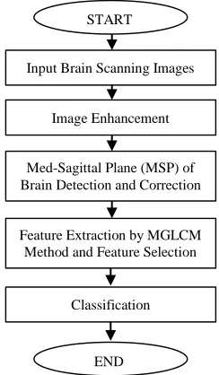
Figure 1: Flow chart of the proposed algorithm.
3.1 Data Collection
Data collection is an important step in this study. T2 weighted images in axial viewing of 165 patients were collected from the MRI Unit of Al-Kadhimiya Teaching Hospital in Iraq. Each patient has 32 slices with a slice resolution of (432×512 pixels). T2 weighted modality is used in this study for detecting brain tumors because most of the brain tumors appear hyperintense relative to normal brain tissue [14]. The dataset was collected using a SIEMENS MAGNETOM Avanto 1.5 Tesla scanner and PHILIPS Achieva 1.5 Tesla scanner. The provided dataset consists of tumors with different sizes, shapes, locations, orientations and types.
3.2 Image Preprocessing
The preprocessing step includes implementing three main algorithms on the slices of the MRI brain scans as preparation for the features extraction step. t includes resizing the dimensions of MRI slices, image enhancement by the Gaussian filter and MRI intensity normalization – necessary because of intra-scan and inter-scan image intensity variations [1, 10, 15].
3.3 Mid- Sagittal Plane Detection and Correction
MSP identification is an important initial step in brain image analysis as it provides an initial estimation of the brain's pathology assessment and tumor detection [12]. The human brain is divided into two hemispheres that have approximately bilateral symmetry around the MSP. This means that most of the structures in one side of the brain have a counterpart on the other side with similar shape and location. The two hemispheres are separated by the longitudinal fissure that represents a membrane between the left and right hemispheres [11]. The MSP extraction methods can be divided into two groups [11, 16] - Content-based methods that are based on finding a plane that maximizes a symmetry measure between both sides of the brain [11] and Shape-based methods that use the inter-hemispheric fissure as a simple landmark to extract and detect the MSP [16].
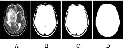
In this study, we are interested in determining the orientation of the patient’s head instead of depending on measuring the symmetry to identify the brain MSP as we are using the Principal Components Analysis (PCA) method to compute the distinctive principle axes that are orthogonal to each other. Those axes are used to characterize the patient’s head by representing the spatial distribution of the mass [16]. The proposed algorithm includes five steps. The first step separates the brain from the background by using the histogram thresholding approach because the background normally has a much higher number of unavailing pixels [1]. The second step also uses the holes filling morphological operator to fill the holes that are defined as a background region of a binary image and surrounded by connected borders of foreground [17] as shown in Fig. 2.
Input Brain Scanning Images
END START
Image Enhancement
Med-Sagittal Plane (MSP) of Brain Detection and Correction
Feature Extraction by MGLCM Method and Feature Selection
Figure 2: An example for MRI brain scanning image segmentation, A) Original MRI image, B) Segmented MRI image with threshold equal to 25, C) Dilated MRI image, and
D) Filled holes image.
The third step determines the orientation of the patient's head using PCA. The PCA method essentially attempts to transfer the coordinates of the original data to a new coordinates system such that the maximum variation in the data comes to lie on the first coordinate. This is known as the first principal component. The second maximum variation in the data lies on the second coordinate and so on [17]. The new coordinates of the given data are estimated by calculating the eigenvectors which point in the direction of the new dataset coordinates. The desirable coordinate that has the highest eigenvalues, passing through the maximum variation of data, represent the orientation of the patient's head [17]. The angle θ between the X-axis and X’-axis represent the degree of skewness of the patient’s head during the MRI test as shown in Fig. 3 and is calculated using Equation 1.
𝜃 = 𝑡𝑎𝑛−1𝑉2
𝑉1 1
Where, V1 and V2 are the eigenvectors which are related to the maximum eigenvalues.
Figure 3: Original and new coordinates of a patient's head.
The fourth step is a Geometrical transformation which is widely used in computer graphic and image analysis. It includes two basic steps. First, the pixel coordinates transformation and second, the brightness interpolation [17]. In this study, it is used to rotate and correct the patient's head after the degree of wobbling is calculated in the previous step. The fifth step is the positioning of the patient’s head in the centre of the MRI image because identifying the brain’s abnormality depends essentially on measuring the symmetry between the two brain’s hemispheres.
The MRI brain slices of each patient have the same degree of skewness; therefore the MSP detection and correction algorithm is implemented on a single slice instead of using all slices to avoid computational complexity. The preferable slice for implementing the MSP detection and correction algorithm is the slice which is located in the middle of all the slices. The MRI brain scanning image is divided evenly into two halves, each half containing one brain hemisphere. Hence after correcting and rotating the patient’s head, it is easy to position the brain’s MSP exactly in the middle of the MRI scanning image by shifting the patient’s head either left or right. Eventually, the brain image is centralized and skewness free.
4.
Proposed Feature Extraction Method
(MGLCM) method. The texture features will also be used to measure statistically the similarity between the two separated hemispheres of the brain. A prior preprocessing algorithms that should be taken to prepare the MRI brain scanning image for texture features extraction by the proposed method is used.
4.1 MRI Brain Scanning Image Preparing
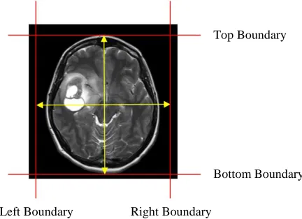
[image:6.612.230.446.236.393.2]This step includes the implementation of a set of image preprocessing algorithms to prepare and make the MRI brain scanning images more appropriate for implementing the MGLCM method. The input for this step is a corrected MRI brain scanning image, and the output image includes only the patient’s head with dimensions of (512×512) pixels. Initially, the MRI image is cropped from the upper margin of the image to the upper boundary of the skull. The same procedure is then used done for cropping the MRI image from the bottom margin of the image to the bottom boundary of the skull. The left and right boundaries can then be identified by measuring the distance between the upper and bottom boundaries such that, the left and right boundaries are away from the middle of the MRI image which denotes the MSP of the brain, by a half distance between the top and bottom boundaries as shown in Fig. 4. Finally, every cropped MRI brain scan image is resized to (512×512) pixels before implementing the MGLCM method.
Figure 4: MRI brain scanning image cropping.
4.2 Modified Grey Level Co-occurrence Matrix MGLCM Algorithm
MGLCM is a second order statistical method. It is proposed in this study to generate texture features of MRI brain scans by computing the joint frequencies of all pairwise combinations of the grey levels configuration of each pixel in the left hemisphere, which is considered as a reference pixel, with one of the nine opposite pixels in the right hemisphere according to the nine offsets θ=(45,45),(0,45),(315,45),(45,0),(0,0),(315,0),(45,315),(0,315),(315,315), and one distance d=1, as shown in Fig. 5. Subsequently, because each pixel on the left hemisphere has nine opposite pixels on the right hemisphere, nine co-occurrence matrices are obtained for each MRI brain scanning image.
Thereafter, each co-occurrence matrix is normalized by the sum of all its elements to calculate the co-occurrence relative frequency between the grey levels of joint pixels in the brain hemispheres. The nine co-occurrence matrices are defined using Equation 2.
𝑃(𝑖, 𝑗)(𝜃1,𝜃2)=
1
2562∑ ∑ {
1 , 𝑖𝑓 𝐿(𝑥, 𝑦) = 𝑖 𝑎𝑛𝑑 𝑅(𝑥 + ∆𝑥, 𝑦 + ∆𝑦) = 𝑗
0 , 𝑂𝑡ℎ𝑒𝑟𝑤𝑖𝑠𝑒
2
256
𝑦=1 512
𝑥=1
Top Boundary
Bottom Boundary
Figure 5: How a reference pixel relates with its opposite nine pixels.
Where L and R denote the left and right hemispheres respectively and both of them have a size of (512×256) pixels. P is the resultant co-occurrence matrix. ∆x and ∆y are changed dependent upon the directions of the measured matrix with the following rules used:
if θ1= 0 and θ2= 0 then ∆x = 0 and ∆y = 0,
if θ1= 0 and θ2= 45 then ∆x = −1 and ∆y = 0, if θ1= 0 and θ2= 315 then ∆x = 1 and ∆y = 0,
if θ1= 45 and θ2= 0 then∆x = 0 and ∆y = 1, if θ1= 315 and θ2= 0 then ∆x = 0 and ∆y = −1,
if θ1= 45 and θ2= 45 then ∆x = −1 and ∆y = +1, if θ1= 315 and θ2= 45 then ∆x = −1 and ∆y = −1,
if θ1= 315 and θ2= 45 then ∆x = −1 and ∆y = −1,
if θ1= 315 and θ2= 315 then ∆x = 1 and ∆y = −1,
if θ1= 45 and θ2= 315 then ∆x = 1 and ∆y = 1.
The resultant co-occurrence matrices are approximately symmetric around the forward diagonal of the matrix for a healthy brain, and asymmetrical for pathological patients. Fig. 6 shows two examples of normal and abnormal MRI brain scanning and the corresponding co-occurrence matrix at angle (0, 0) of a normal and an abnormal brain scanning.
Figure 6: A) MRI normal brain scanning image, B) MRI abnormal brain scanning image, C) MGLCM of normal brain scanning and D) MGLCM of abnormal brain scanning.
[image:7.612.191.413.507.660.2]symmetry represents the main indicator to detect pathological brains.
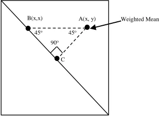
[image:8.612.256.416.111.229.2]1-Weighted mean descriptor is proposed in this study to detect the irregularity of the MRI brain scanning image by calculating the nearest distance between the weighted mean to the diagonal of co-occurrence matrix as shown in Fig. 7.
Figure 7: Weighted mean representation in co-occurrence matrix.
It is high when there is any abnormality in the MRI brain scanning image and low when there is normal brain scanning and defined using Equation 3 and Equation 4:
𝑥 = 1
2562∑ ∑ 𝑖. 256
𝑗=1 256
𝑖=1
𝑃(𝑖, 𝑗) 3
𝑦 = 1
2562∑ ∑ 𝑗. 256
𝑗=1 256
𝑖=1
𝑃(𝑖, 𝑗) 4
Where x and y are the coordinates of weighted mean in the co-occurrence as given in Equation 5.
𝑊𝑒𝑖𝑔ℎ𝑡𝑒𝑑 𝑚𝑒𝑎𝑛(𝐴,𝐵)= |𝑦 − 𝑥| sin 45𝑜 5
2-Weighted distance descriptor is also proposed in this study to detect the irregularity of the MRI brain scanning image by multiplying each coefficient in the co-occurrence matrix by the nearest distance d to the diagonal as shown in Fig. 8. It is high with abnormal brain scanning and low with normal brain scanning and defined using Equation 6 and Equation 7.
𝑢𝑝𝑡𝑟𝑎𝑛𝑔.= ∑ ∑ 𝑑𝑖𝑗. 𝑃(𝑖, 𝑗) 𝑗
𝑖
6
Where, i and j are the element's coordinates of co-occurrence matrix that are located in the upper triangular of the matrix.
𝑙𝑜𝑤𝑡𝑟𝑎𝑛𝑔.= ∑ ∑ 𝑑𝑖𝑗. 𝑃(𝑖, 𝑗) 𝑗
𝑖
7
Where, i and j are the element's coordinates of co-occurrence matrix that are located in the lower triangular of the matrix as shown in Equation 8.
𝑊𝑒𝑖𝑔ℎ𝑡𝑒𝑑 𝑑𝑒𝑠𝑡𝑎𝑛𝑐𝑒 = |𝑢𝑝𝑡𝑟𝑎𝑛𝑔.− 𝑙𝑜𝑤𝑡𝑟𝑎𝑛𝑔.| 8
Subsequently, there are 190 predictors that are extracted from 9 offsets for each MRI brain scanning. A(x, y)
B(x,x)
C 90o
45o
45o
improving the accuracy, efficiency and scalability of the classification process [20]. Features Transformation is the process of transforming all extracted features by normalization, into new forms that are more appropriate for the classification process to prevent features with large ranges outweighing those from smaller ones. In this study, the min-max normalization approach is used to perform a linear transformation on the extracted features whilst preserving the relationships between the original features [20].
Relevance Analysis is the process of identifying and removing irrelevant and redundant features that do not contribute to the classification process and to reduce computational complexity by transforming high-dimensional data into a meaningful representation of the reduced dimensionality. It also contributes to improving training of the classifier to be faster, more effective and more accurate [21, 22]. A redundant feature is defined as one that it is highly correlated with one or more of the other features, provided both of them are relevant, while the irrelevant predictor can be removed without affecting the classification performance. As stated by Hall [21], “a good feature subset is one that contains features that are highly correlated with the group and uncorrelated with each other”.
In this study, stepwise analysis of variance ANOVA is used. It is a robust statistical technique used for data analysis and for detecting the level of significance of each predictor in the feature space based on calculating whether differences exist between two or more group means by analyzing the within-group and between-group variance. It predicts the significance of a predictor using F-statistic and P-values where the F-statistic is defined as the ratio of between-group variance to the within-group variance. The predictor that has the highest significant variation between classes has a high F-statistic value and a small P-value. From the ANOVA table, when the P-value for the F-statistic value is less than the critical value α, then the predictor will be significant. The critical value α is proposed and fixed by Fisher [23]. He suggested the idea of a conventional probability for accepting or rejecting the hypothesis and it was one in twenty (0.05 or 5%). Consequently, the predictor will be significant when P<0.05, very significant when P<0.01, and highly significant when P<0.001.
5.
Classification
Classification is the process of sorting objects in an image into separated classes, and represents the final step of image processing. Three classifiers are applied and the results are compared. These classifiers are Linear Discriminant Analysis (LDA), Support Vector Machine (SVM), and Multi-layer Perceptron Neural Network (MLP). Training samples are randomly selected. A 10-folded cross-validation is used to validate the robustness of our proposed system. Cross-validation also helps to prevent overfitting.
6.
Experimental Results
To evaluate the proposed algorithms of this study a set of examples will be implemented using these algorithms.
6.1 MSP Detection and Correction Results
Fig. 9 shows the result of MSP detection and correction of the three MRI brain scanning images which are shown in different orientation in the first row. In the second row, the scans are corrected and aligned in the middle of image. The MRI image shown in Fig. 10, is re-sampled using the Geometric Rotator system object in the MATLAB Image Processing Toolkit [24], to rotate the patient’s head with yaw angles from -10 to 10 degrees in 5 degree intervals. The proposed algorithm is evaluated by comparing our results with the proposed algorithms in [16] as shown in Table I. It is noted that there is a significant difference in the mean squared error (MSE) between both algorithms, and the performance of our algorithm outperforms those proposed in [16].
6.2 Classification Results
Figure 9: MSP detection and correction of three pathological patients.
[image:10.612.189.417.258.315.2]-10 -5 0 5 10
Figure 10: Re-sampling of one slice from the axial MRI brain scanning image with varied rotation angles.
TABLE I:NUMERICAL RESULTS OF DETECTING YAW ANGLE
Yaw Angle -10 -5 0 5 10 MSE
Detected Yaw Angle -9.1 -4.7 0.5 5.4 10.5 0.3
[16] -8.5 -3 1.25 6.5 11.2 2.87
Additionally, the performance of the features which were extracted by MGLCM was compared with the Gabor wavelet features that were applied with five different scales and eight orientations using a window size of (33×33). The length of the Gabor feature vector was 655360. The achieved classification accuracy by the three classifiers was 90% for SVM, 62.5% for LDA and 87.4% for MLP. As shown in Fig. 11, the classification accuracies of the texture features that were extracted using MGLCM are higher than those extracted using GLCM and Gabor wavelet features in all classifiers.
Figure 11: A comparison between MGLCM and GLCM classification accuracy.
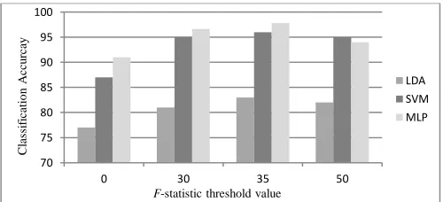
After implementing the stepwise analysis of the variance ANOVA method for relevance analysis, in this study, the critical value α is set to 0.001 in order to obtain highly significant features. The assessment of the features will depend on both F-statistic value and P-value, as it is not enough that a predictor has a P-value that is less than 0.001 but it should also have a high F-statistic value. Therefore a threshold value will be used to evaluate the significance of the predictors in addition to P-value. Once the F-statistic threshold value is set to zero, all predictors in the features vector will be selected. When the F-statistic threshold value is increased, the number of selected predictors decreases and the features vector is reduced. Therefore, to choose the optimal F-statistic threshold value, the classification accuracy of the three classifiers should be examined and evaluated. Different F-statistic threshold values are tested at each run when we measure the number of predictors which have an F-statistic
40 60 80 100
LDA SVM MLP
C
la
ss
if
ic
ati
o
n
A
cc
u
rc
ay GLCM
MGLCM
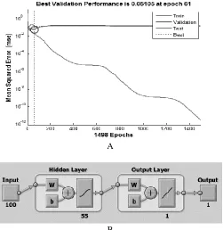
[image:10.612.154.459.374.420.2] [image:10.612.183.431.502.601.2]Fig. 12 shows that the classification accuracy of the three classifiers has improved and reached the maximum value when the F-statistic threshold value is set to 35. It also shows that the average performance of LDA and SVM models were 83% and 96% respectively. The transfer function used in the MLP network was the tangent function and the training function. To update the weights and bias values, the scaled conjugate gradient method (trainscg) that is suggested by MATLAB to be faster than the default function (trainlm) for larger datasets, is used. The training of the MLP network with 100 input layer neurons, 55 hidden layer neurons and single output layer is shown in Fig. 13. The average performance of the MLP network was 97.8± 0.1% and sensitivity and specificity rates were 98.1± 0.3% and 97.6± 0.4% respectively. Additionally, there was just one non-pathological patient that was classified incorrectly as pathological and three pathological patients that were classified incorrectly as non-pathological.
[image:11.612.100.511.108.188.2]Subsequently, the number of predictors in the feature vector is reduced from 190 to 100 predictors with 90 predictors discarded and considered as irrelevant or redundant features. Eleven relevant and significant features for each angle of the MGLCM are chosen by the ANOVA method namely: contrast, correlation, dissimilarity, sum of square variance, sum average, sum variance, difference entropy, information measure of correlation 1, inverse difference normalized (IDN), inverse difference moment normalized (IDMN) and weighted distance in addition to the cross correlation.
Figure 12: The optimal F-statistic threshold value.
The ANOVA method was also applied on the texture features which were extracted by the traditional GLCM. The best classification accuracy was achieved when the F-statistic threshold value was 35, such that the selected texture features were auto correlation, cluster prominence, cluster shade, sum of square variance, sum variance and cross correlation. The maximum classification accuracy of MLP, SVM and LDA were 92%, 90% and 79% respectively. It can be clearly seen that the classification accuracy of the used classifiers were significantly higher when using MGLCM method than GLCM as shown in Fig. 14.
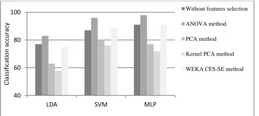
The performance of ANOVA is validated by comparing its results against those obtained by other techniques for feature selection mainly PCA and Kernel PCA methods [22, 25]. Table III and Table IV show the results when using PCA and Kernel PCA respectively as feature selection and reduction methods with the same dimensions that were used with ANOVA (127, 100 and 55) and the results of classification accuracy of the same classifiers that were used previously in this study.
70 75 80 85 90 95 100
0 30 35 50
C
la
ss
if
ic
ati
o
n
A
cc
u
rc
ay
F-statistic threshold value
LDA SVM MLP
threshold value predictors Accuracy Accuracy Size of
hidden layer Accuracy
30 127 81% 95% 60 96.6%
35 100 83% 96% 55 97.8%
[image:11.612.181.431.379.493.2]A
[image:12.612.182.433.52.310.2]B
[image:12.612.184.426.354.467.2]Figure 13: A) MLP network structure and B) The performance of MLP network.
Figure 14: A comparison between MGLCM and GLCM regard classification accuracy when using ANOVA method.
TABLEIII
CLASSIFICATION ACCURACY FOR THE THREE CLASSIFIERS WITH PCA METHOD FOR FEATURE SELECTION.
No. of selected predictors
LDA Accuracy
SVM Accuracy
MLP Size of hidden
layer Accuracy
127 65% 78% 65 66%
100 63% 80% 55 77%
55 63% 78% 25 78%
TABLEIV
CLASSIFICATION ACCURACY FOR THE THREE CLASSIFIERS WITH KERNEL PCA
METHOD FOR FEATURE SELECTION.
No. of selected predictors
LDA Accuracy
SVM Accuracy
MLP
Size of hidden layer Accuracy
127 60% 81% 65 62%
100 61% 74.5% 55 67%
55 58% 76% 25 72%
40 50 60 70 80 90 100
LDA SVM MLP
C
la
ss
if
ic
ati
o
n
A
cc
u
ra
cy
GLCM
[image:12.612.137.477.654.727.2]TABLEV
CLASSIFICATION ACCURACY FOR THE THREE CLASSIFIERS WITH
WEKACFS-SE METHOD FOR FEATURE SELECTION.
No. of selected predictors
LDA Accuracy
SVM Accuracy
MLP
Size of hidden layer Accuracy
6 75% 89% 3 91%
[image:13.612.135.483.149.196.2]Fig. 15 summarizes the behavior of the implemented features selection methods and shows that the behaviour of ANOVA outweighs the performance of the other techniques for detecting the most relevant predictors.
Figure 15: Performance of the implemented methods for feature selection.
7.
Discussion
Since visual diagnosis of the MRI scans is subjective and depends on the expertise of the radiologist, texture analysis has been widely studied for improving the diagnosis of MRI brain scans. In this study, 19 co-occurrence statistics which are most popular and common in previous studies, in addition to two additional texture features which were proposed in this study, were extracted from nine MGLCM matrices to discriminate brain abnormalities. Only 11 co-occurrence statistics in addition to cross correlation predictor were chosen as the most significant features by ANOVA. The weighted distance feature proposed in this study, was included within these 11 co-occurrence statistics and was chosen by ANOVA as a significant feature. The experimental results of the proposed algorithm are compared with previous studies as shown in Table VI.
TABLEVI
COMPARISON WITH PREVIOUS PROPOSED METHODS
Reference Features methods No. of Patients Classifier Accuracy
[10]
- First-order statistical
- GLCM (4 orientations and 2 distances) - GLRLM (4 orientations)
- HOG - LBP
25 SVM 97.4%
[14] -Searching about pathological area by symmetry checking 203 SVM 91.15%
[19] -GLCM (4 orientations and 10 distances) 436 LDA 87%
Proposed
System -MGLCM (9 orientations and 1 distance) 165 MLP 97.8%
The authors in [10] used five methods for feature extraction; first-order statistical features, GLCM with four orientations (0o, 45o, 90o and 135o) and two distances (1 and 2), GLRLM with four orientations (0o, 45o, 90o and 135o), a histogram of oriented gradient features HOG and linear binary pattern features LBP. The feature vector included 475 predictors. The dataset included 25 patients. A classification accuracy of 97.4% was achieved by SVM. If we consider that there were 5 feature extraction methods, and the processing time of first-order statistical method, HOG and LBP was 3n, the GLCM required 8n because there
40 60 80 100
LDA SVM MLP
Cl
as
si
fi
ca
ti
o
n
a
cc
u
ra
cy
Without features selection
ANOVA method
PCA method
Kernel PCA method
[image:13.612.180.443.243.361.2] [image:13.612.50.567.532.664.2]were four orientations and two distances and the GLRLM required 4n because there were four orientations. Then, the total processing time is TP=15n. By using the big-O notation, we could write Tf = O(15n), which indicates that the complexity of the previous algorithm depends mainly on the number of feature extraction methods.
The authors in [19] used the GLCM method for feature extraction to classify breast ultrasound images (BUS) with 22 predictors computed from four co-occurrence matrices with orientations (0o, 45o, 90o and 135o), ten distances (1-10 pixels) and six quantization levels (8, 16, 32, 64, 128 and 256). To reduce the dimensionality of the feature space, the texture descriptors of the same distance were averaged over all orientations from 880 to 220. Additionally, mutual information (MI) is used for evaluating the quality of the features subset. The maximum classification accuracy was achieved by the LDA classifier at 87% for classifying 436 BUS images. The selected predictors were feature/θ/d; correlation I/90/8, cluster prominence/0/1, correlation II/90/8, contrast/90/1, correlation I/90/9, difference variance/90/1, correlation II/90/9, correlation I/90/2, correlation I/90/7, inverse difference moment normalize/90/1, correlation II/90/7, correlation I/90/10, correlation I/90/6, correlation II/90/10, correlation II/90/6, correlation I/90/5 and inverse difference moment normalize/90/1. The total processing time is TP=9n and using the big-O notation, we could write Tf = O(9n).
The automated screening algorithm in this study depends essentially on the single proposed method for texture feature extraction MGLCM with nine orientations. The significant features were selected using the ANOVA method and were reduced to 100 predictors. Over the entire dataset which included 165 patients, the average achievable accuracy was 97.8% by using MLP. The big-O notation of the proposed algorithm is Tf = O(9n).
8.
Conclusion
An automated screening algorithm of MRI brain scanning images is developed to identify brain abnormality. This algorithm helps clinicians to improve the accuracy of the diagnosis and to reduce the diagnosing time. It is observed that the statistical texture features which were extracted by MGLCM are sufficient to discriminate the pathological patients from non-pathological patients by using T2 weighted MRI images because most of the brain tumors appear hyperintense in these images relative to normal brain tissue. It is also noted, that the achieved accuracy with low computational complexity demonstrates the efficiency of the proposed method for features extraction and its independence from the atlas registration method. A further advantage of our approach is that it uses a single MRI scan modality (T2 weighted image). The MGLCM gives high performance and accuracy in discriminating the normality and abnormality of the brain. However, the method is computationally expensive and memory requirements represent disadvantage.
Acknowledgement
We would like to thank the reviewers for their insightful comments on the paper, as these comments led to improve the quality of the paper and the MRI Unit of Al Kadhimiya Teaching Hospital in IRAQ for providing us with the MRI brain scanning images dataset.
Appendix
The 19 texture features used in our work were extracted from the MGLCM, these features are summarized below [19]:
𝐴𝑢𝑡𝑜𝑐𝑜𝑟𝑟𝑒𝑙𝑎𝑡𝑖𝑜𝑛𝑝𝑟𝑒𝑑𝑖𝑐𝑡𝑜𝑟 = ∑ ∑(𝑖 . 𝑗)𝑃(𝑖, 𝑗)
𝑁
𝑗=0 𝑁
𝑖=0 1
𝐶𝑜𝑛𝑡𝑟𝑎𝑠𝑡 = ∑ 𝑛2{∑ ∑ 𝑃(𝑖, 𝑗)
𝑁
𝑗=0 𝑁
𝑖=0
}
𝑛−1
𝑛=0
𝑤ℎ𝑒𝑟𝑒𝑛 = |𝑖 − 𝑗
2
𝐶𝑜𝑟𝑟𝑒𝑙𝑎𝑡𝑖𝑜𝑛 = ∑ ∑ 𝑃(𝑖, 𝑗)(𝑖 − 𝜇𝑥)(𝑗 − 𝜇𝑦)
𝜎𝑥𝜎𝑦
𝑁−1
𝑗=0 𝑁−1
𝑖=0 3
𝐸𝑛𝑡𝑟𝑜𝑝𝑦 − ∑ ∑ 𝑃(𝑖, 𝑗) log 𝑃(𝑖, 𝑗)
𝑁−1
𝑗=0 𝑁−1
𝑖=0 4
𝐸𝑛𝑒𝑟𝑔𝑦 = ∑ ∑ 𝑃(𝑖, 𝑗)2
𝑁−1
𝑗=0 𝑁−1
𝑆𝑢𝑚𝑜𝑓𝑠𝑞𝑢𝑎𝑟𝑒𝑣𝑎𝑟𝑖𝑎𝑛𝑐𝑒 = ∑ ∑(𝑖 − 𝜇)2. 𝑃(𝑖, 𝑗) 𝑁−1
𝑗=0 𝑁−1
𝑖=0 8
𝐶𝑙𝑢𝑠𝑡𝑒𝑟𝑠ℎ𝑎𝑑𝑒 = ∑ ∑(𝑖 + 𝑗 − 𝜇𝑥− 𝜇𝑦)3𝑃(𝑖, 𝑗)
𝑁−1
𝑗=0 𝑁−1
𝑖=0 9
𝐶𝑙𝑢𝑠𝑡𝑒𝑟𝑝𝑟𝑜𝑚𝑖𝑛𝑒𝑛𝑐𝑒 = ∑ ∑(𝑖 + 𝑗 − 𝜇𝑥− 𝜇𝑦)4𝑃(𝑖, 𝑗)
𝑁−1
𝑗=0 𝑁−1
𝑖=0 10
𝐼𝑛𝑣𝑒𝑟𝑠𝑒𝑑𝑖𝑓𝑓𝑒𝑟𝑒𝑛𝑐𝑒𝑛𝑜𝑟𝑚𝑎𝑙𝑖𝑧𝑒𝑑 = ∑ ∑ 1
1 +|𝑖 − 𝑗|𝑁 𝑃(𝑖, 𝑗)
𝑁−1
𝑗=0 𝑁−1
𝑖=0 11
𝐼𝑛𝑣𝑒𝑟𝑠𝑒𝑑𝑖𝑓𝑓𝑒𝑟𝑒𝑛𝑐𝑒𝑚𝑜𝑚𝑒𝑛𝑡𝑛𝑜𝑟𝑚𝑎𝑙𝑖𝑧𝑒𝑑 = ∑ ∑ 𝑃(𝑖, 𝑗)
1 +(𝑖 − 𝑗)𝑁 2
𝑁−1
𝑗=0 𝑁−1
𝑖=0 12
𝑆𝑢𝑚𝑎𝑣𝑒𝑟𝑎𝑔𝑒𝑝𝑟𝑒𝑑𝑖𝑐𝑡𝑜𝑟 = ∑ 𝑖𝑃𝑖+𝑗(𝑖, 𝑗)
2𝑁−1
𝑖=1
13
𝑆𝑢𝑚𝑒𝑛𝑟𝑜𝑝𝑦𝑝𝑟𝑒𝑑𝑖𝑐𝑡𝑜𝑟 = − ∑ 𝑃𝑖+𝑗(𝑖, 𝑗)
2𝑁−1
𝑖=1
𝑙𝑜𝑔 𝑃𝑖+𝑗(𝑖, 𝑗) 14
𝑆𝑢𝑚𝑣𝑎𝑟𝑖𝑎𝑛𝑐𝑒𝑝𝑟𝑒𝑑𝑖𝑐𝑡𝑜𝑟 = ∑ (𝑖 − 𝑠𝑢𝑚𝑒𝑛𝑡𝑟𝑜𝑝𝑦)2𝑃
𝑖+𝑗(𝑖, 𝑗)
2𝑁−1
𝑖=1
15
𝐷𝑖𝑓𝑓𝑒𝑟𝑒𝑛𝑐𝑒𝑒𝑛𝑟𝑜𝑝𝑦𝑝𝑟𝑒𝑑𝑖𝑐𝑡𝑜𝑟 = − ∑ 𝑃𝑖−𝑗(𝑖, 𝑗)
𝑁−1
𝑖=0
𝑙𝑜𝑔 𝑃𝑖−𝑗(𝑖, 𝑗) 16
𝐼𝑛𝑓𝑜𝑟𝑚𝑎𝑡𝑖𝑜𝑛𝑚𝑒𝑎𝑠𝑢𝑟𝑒𝑜𝑓𝑐𝑜𝑟𝑟𝑒𝑙𝑎𝑡𝑖𝑜𝑛𝐼 =𝐻𝑋𝑌 − 𝐻𝑋𝑌1
𝑚𝑎𝑥 (𝐻𝑋, 𝐻𝑌) 17
𝐼𝑛𝑓𝑜𝑟𝑚𝑎𝑡𝑖𝑜𝑛𝑚𝑒𝑎𝑠𝑢𝑟𝑒𝑜𝑓𝑐𝑜𝑟𝑟𝑒𝑙𝑎𝑡𝑖𝑜𝑛𝐼𝐼 = √1 − 𝑒(−2(𝐻𝑋𝑌2−𝐻𝑋𝑌)) 18
𝑀𝑎𝑥𝑖𝑚𝑢𝑚𝑝𝑟𝑜𝑏𝑎𝑏𝑖𝑙𝑖𝑡𝑦𝑝𝑟𝑒𝑑𝑖𝑐𝑡𝑜𝑟 = 𝑚𝑎𝑥𝑖,𝑗𝑃(𝑖, 𝑗) 19
References
[1] N. Nabizadeh, "Automated Brain Lesion Detection and Segmentation Using Magnetic Resonance Images," PhD Thesis, Department of Electrical and Computer Engineering, University of Miami, USA, 2015.
[2] B. Saha, N. Ray, R. Greiner, A. Murtha, and H. Zhang, "Quick detection of brain tumors and edemas: A bounding box method using symmetry", Computerized Medical Imaging and Graphics, vol. 36, No 2, pp. 95-107, 2012.
[3] D. Mortazavi, A. Z. Kouzani, and H. Soltanian-Zadeh, "Segmentation of multiple sclerosis lesions in MR images: a review", Neuroradiology, vol. 54, No 4, pp. 299-320, 2012.
[4] B. H. Menze, A. Jakab, S. Bauer, J. Kalpathy-Cramer, K. Farahani, J. Kirby, et al., "The Multimodal Brain Tumor Image Segmentation Benchmark (BRATS)", IEEE Transactions on Medical Imaging, vol. 34, Issue 10, pp. 1993-2024, 2015.
[5] R. Fathi, L. Matti, H. Al-Salih, and D. Godbold, "Environmental pollution by depleted uranium in Iraq with special reference to Mosul and possible effects on cancer and birth defect rates," Medicine, Conflict and Survival, vol. 29, No 1, pp. 7-25, 2013.
[6] A. Kharrat, G. Karim, M. Ben Messaoud, N. Benamrane, and M. Abid, "A Hybrid Approach for Automatic Classification of Brain MRI Using Genetic Algorithm and Support Vector Machine," Leonardo Journal of Sciences, issue 17,. pp. 71-82, 2010.
Extraction from Biomedical Images," Journal of Medical Engineering, vol. 2013, pp. 1-13, 2013.
[9] J. Sachdeva, V. Kumar, I. Gupta, N. Khandelwal, and C. Ahuja, "Segmentation, Feature Extraction, and Multiclass Brain Tumor Classification," Swetswise, vol. 26, No 6, pp. 1141-1150, 2013.
[10] N. Nabizadeh and M. Kubat, "Brain tumors detection and segmentation in MR images: Gabor wavelet vs. statistical features," Computers & Electrical Engineering, vol. 45, pp. 286–301, 2015.
[11] G. Ruppert, L. Teverovskiy, Y. Chen-Ping, X. Falcao, and L. Yanxi, "A new symmetry-based method for mid-sagittal plane extraction in neuroimages", International Symposium on Biomedical Imaging: From Nano to Macro, Chicago, IL, 2011, pp. 285-288.
[12] S. Jayasuriya and A. Liew, "Symmetry plane detection in neuroimages based on intensity profile analysis", The International Symposium on Information Technology in Medicine and Education (ITME), pp.599-603, Australia 2012. [13] U. Stańczyk and L. Jain, Feature Selection for Data and Pattern Recognition: An Introduction. In U. Stańczyk and L.
Jain (Eds), Feature Selection for Data and Pattern Recognition, Springer Series on Studies in Computational Intelligence vol. 584, pp: 1-7, Berlin Heidelberg: Springer, 2015.
[14] P. Dvořák, W. Kropatsch, and K. Bartušek, "Automatic brain tumor detection in t2-weighted magnetic resonance images," Measurement Science Review, vol. 13, No 5, pp. 223-230, 2013.
[15] S. Tantisatirapong, "Texture analysis of multimodal magnetic resonance images in support of diagnostic classification of childhood brain tumours," PhD Thesis, School of Electronic, Electrical and Computer Engineering, University of Birmingham, 2015.
[16] Y. Liu and R. Collins, "Automatic Extraction of the Central Symmetry (MidSagittal) Plane from Neuroradiology Images," Technical report, CMU-RI-TR-96-40, Robotics Institute, Carnegie Mellon University,1996.
[17] M. Sonka, V. Hlavac, and R. Boyle, Image Processing, Analysis, ans Machine Vision, third edition ed., 2008.
[18] M. Haralick, K. Shanmugam and I. H. Dinstein, "Textural Features for Image Classification,", IEEE Transactions on Systems, Man and Cybernetics, vol. SMC-3, Issue 6, pp. 610-621, 1973.
[19] W. Gomez, W. Pereira, and A. Infantosi, "Analysis of Co-Occurrence Texture Statistics as a Function of Gray-Level Quantization for Classifying Breast Ultrasound", IEEE Transactions on Medical Imaging, vol. 31, issue 10, pp. 1889-1899, 2012.
[20] J. Han and M. Kamber, Data Mining: Concepts and Techniques. USA: Diane Cerra, 2006.
[21] M. Hall, "Correlation-based Feature Selection for Machine Learning," PhD Thesis, Department of Computer Science, University of Waikato, NewZealand, 1999.
[22] P. Van der Maaten, "An Introduction to Dimensionality Reduction Using Matlab," Technical Report, Report MICC 07-07 , Faculty of Humanities & Sciences, Maastricht University, The Netherlands, 2007-07.
[23] G. Quinn and M. Keough, Experimental Design and Data Analysis for Biologists, Cambridge Press, UK, 2002. [24] Matlab, "The Math Works kit," ed, 2013.
[25] Matlab Toolbox for Dimensionality Reduction. (2015). Available: http://lvdmaaten.github.io/drtoolbox/
Ali. M. Hasan is currently a Ph.D. candidate in the School of Computing, Science and Engineering at the University of Salford,
UK. Prior to his PhD studies, he was a lecturer in the College of Medicine at Al-Nahrain University, Iraq. He can be contacted at: [email protected]; [email protected].
Farid Meziane is a professor in Data and Knowledge Engineering in the School of Computing, Science and Engineering at the