An Image Denoising Method Based on Geodesic Distance

2017 2nd International Conference on Computer, Mechatronics and Electronic Engineering (CMEE 2017) ISBN: 978-1-60595-532-2

An Image Denoising Method Based on Geodesic Distance

Yin-long WANG

and Yong-chao ZHOU

1

The 5th Department of Army Engineering University, Shijiazhuang China

2

The Special Equipment Repair Shop, Tieling China

*Corresponding author

Keywords: Image denoising, Geodesic, PSNR.

Abstract. In this paper, an image denoising method based on geodesic distance is proposed. Different from the denoising method in the traditional Euclidean space, this image denoising method measures the similarity between two pixels in the image according to their geodesic distance. The point in the manifold is a Gaussian model constructed by an area in the image. The geodesic distance between the models represents the difference in the average grayscale intensity and in the abundance of details of the two image regions. This makes the difference in the average gray intensity and in the abundance of details of the regions as the similarity between the pixels, and can more accurately measure the similarity between pixels. Experiments show that this method improves the image denoising effect while still keeping the image details well.

Introduction

Because Gaussian noise seriously affects the visual effect of the image and affects the next step of image processing, it is necessary to reduce the Gaussian noise by using the appropriate method before performing feature extraction and image segmentation. At present, there are many methods of image denoising in space domain, such as statistical method, variational method and partial differential equation method. Information geometry is a new discipline developed in recent years [1] [2] [3]. It is a new theoretical system proposed by modern differential geometry method in Riemannian manifold to study the fields of statistics and information. The information geometry studies a set of probabilistic distribution functions as a whole and investigates the geometric structure information contained in the probability distribution cluster. And the form of the probability distribution function determines the relationship between each probability distribution function and its surrounding probability distribution functions. On the basis of the above principle of information geometry, the Gaussian model is established according to the average gray level and detail abundance of the image region. Based on the spatial distance, the similarity of the average gray intensity and the degree of detail richness in the neighborhood of the pixel is considered so that the denoising ability is improved while the details of the image are maintained [4] [5].

Geodesic

The geodesic lines represent the difference between the average grayscale and the degree of detail abundance between the neighborhoods of the two pixels, and are used to measure the similarity between pixels. In this paper, the geodesic is used in the statistical manifold using Riemann metric to calculate. The following mainly describes the establishment of statistical manifold and the calculation of geodesic [6].

Statistical Manifolds

The neighborhood N around the pixel is an n × n area. According to the gray value of n2 pixel in N, I (x, y) represents the pixel value at (x, y), and the mean value µ and the variance σ2 are by the following equation:

₌

∑ , − , (2)

In the case of each pixel is estimated to have its own Gaussian model with (µ, σ2) as the parameter.

; , =_√ (3) This Gaussian model reflects the distribution of grayscale intensity and detail abundance in the region. The Gaussian distribution of all pixels forms the statistical manifold with (µ, σ2) as the parameter.

Calculation of Geodesic Lines

The statistician Rao proposed to use the Fisher information matrix as a statistical manifold for the Riemannian gauge and to use the geodesic distance to measure the difference between the probability distribution functions, thus opening the statistical geometric study [7]. Fisher degrees is given as following:

gθ = E "#$%&'|)_#)

*

#$%&'|)

#)+ , (4)

The E[ ] represents the mathematical expectation of the random variable, and the Fisher information matrix measures the ability of the two adjacent parameters θ and θ + dθ to be distinguished by the x. The differential distance between adjacent two points p (x | θ) and p (x | θ + dθ) on the statistical manifold can be expressed by the metric:

ds_{= dθ}/_{Gθdθ (5)}

Consider connecting two points θ1θ2 and t1≤ t ≤ t2. The distance between the two points p (x | θ1)

and p (x | θ2) on the statistical manifold given by the curve θ (t) is defined as:

12, 2=3 4567

689 :

;2 567₆₈9 8

8< => (6)

Obviously, the integral distance depends on the selection of the curve θ (t) connecting the two points. The integral distance between p (x | θ1) and p (x | θ2) is usually defined as the minimum length

of all curves θ (t) connecting these two distributions, called the Fisher information distance. The Fisher information distance is the length of the shortest geodesic line connecting two points. The geodesic line is the generalization of the straight line in the Euclidean space in the manifold, and the Fisher information distance is the generalization of the distance of the Euclidean distance in the manifold. For a normal distribution cluster with mean µ and variance σ2, the Fisher information matrix can be expressed as:

;2 = ? 0

0

A (7)

Where θ = (µ, σ2). The statistical manifold with the above metric G (θ) has a hyperbolic structure. We can get the geodesic distance between the normal distribution N1 = (µ1, σ1) and N2 = (µ2, σ2):

B= | C √2

E , F − C √2

E , −F | (8)

B= | C √2

E , F − C √2

E , F | (9)

dHμ, σ, μ, σK = √2lnN<ON

Denoising Method Based on Geodesic Distance

The research of information geometry is based on statistical manifolds, which is composed of clusters of similar probability distributions. We use the gray level information in the pixel neighborhood to estimate the Gaussian model of the pixel. Each pixel in the image has a Gaussian model of the neighborhood estimation, so that all Gaussian models form a statistical manifold. The geodesic distance between the two points on the manifold indicates the similarity between the pixels, the smaller the geodesic distance, the greater the similarity, and the larger the geodesic distance, the smaller the similarity. The image denoising method based on the information geometry is to use the pixels in the neighborhood of the pixels in the image space to be filtered to weight the smoothing. The difference from the traditional denoising method is to use the geodesic to define the similarity weights between pixels. The main steps include:

Step1: Construct the Gaussian model of the pixel according to the mean value µ and the variance σ2

of the pixel gray scale estimation region in the neighborhood around each pixel.

Step2: Integrate all the formed Gaussian distributions into a whole to form a statistical manifold. The mean µ and variance σ2 of the Gaussian distribution are the coordinates of the manifold.

Step3: In the image space, calculate the distance between the pixel to be filtered and the pixel in the neighborhood.

Step4: Calculate the similarity weight using the geodesic to perform weighted smoothing filtering. The similarity weights between the pixel points are determined by the distance between the geodesic distance and the image space, so that the value of the pixel to be filtered is as follows:

P =_Q 3_SR , = (11) Where C(x) is the normalization coefficient, Ω is the filter window centered on x, and I (y) is the value of the pixel. We take the similarity weight R (x, y) as follows:

ωx, y = e|XY|Z (12) The w is the control parameter of the regional geodesic distance. The bigger w is, the smaller is the difference in the similarity weight of each point within the filter window to the point, the better the smoothing effect, but excessive smoothing will make the edge of the image blur; on the contrary, the smaller a is, the difference in the effect of the points within the filter window on the filtering is greater and the smooth effect is worse.

Experimental Result and Analysis

The quality of the de-noising algorithm is usually evaluated according to the image quality after denoising. The amount of image noise removed and the degree of retention of the image structure information are usually indicators of the image quality. In this paper, the PSNR (Peak signal-to-noise ratio) are chosen as the evaluation indexes of image quality after image denoising. The PSNR is difined as [9]:

[\]^ = 20_` 5_√bcdaa 9 (13)

ef\ =_bg ∑ ∑ghPi, j − ki, jl mn

b

on (14)

PSNR measures the algorithm’s ability to denoise. The greater PSNR is the greater the ability to denoise. In order to comprehensively analyze the denoising effect of our algorithm, this paper uses mean filter, and bilateral filter as the contrast. According to the large number of experimental results, the selection range of bilateral filter parameters is given [8] [9].

effect of different algorithms, this paper chooses different images to experiment and uses PSNR to evaluate the filtered denoised images, with the results shown in Table 1.

Table 1. The PSNR of three algorithm.

Noise image

Mean filter

Bilatera l filter

Our method

PSNR

13.21 13.98 14.77 14.91

13.42 13.62 14.43 14.75

13.33 13.72 14.71 14.79

13.28 13.88 14.69 14.82

13.31 13.94 14.78 `14.77

13.55 13.87 14.74 14.80

13.44 13.71 14.81 14.93

13.37 13.88 14.79 14.88

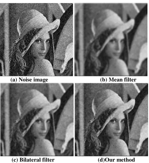
It can be seen from the above quantitative results that the algorithm is stronger than the mean filter in terms of the ability of denoising and maintaining image details. At the same time, when dealing with smoother images as shown in Figure I (Lena image).

(a) Noise image (b) Mean filter

(c) Bilateral filter (d)Our method

Figure 1. Contrast of experimental result.

It’s denoising and edge detail maintaining ability is significantly better than Mean filter and bilateral filter. This is because the algorithm proposed in this paper considers the abundance of the details of the surrounding and also considers the difference between the surrounding gray value.

Conclusion

Reference

[1] Hyvarient A, Karhunen J, Oja Q.Independent Component Analysis [M].New York: Wiley, 2001.

[2] Zang Jun , Wei Z. A Variation Method Basedon Convolution Integral for Image Denoising [J]. Journal of Image and Graphics. 2008, 13(9): 1673-1677.

[3] Tasdizen T. Principal Neighborhood Dictionaries for Nonlocal Means Image Denoising [J]. IEEE Transactions On Image Processing.2009, 18(12): 2649-2660.

[4] Aboshosha, A., Hassan, M., Ashour,M, EI Mashade,M. ImageDenoising Based on Spatial Filters, an Analytical Study[J]. Computer Engineering & Systems, 2009.

[5] Han L, Yong G, Gang Z. Image Denoising Based on Least Squares Support Vector Machines[C]. Proc. of the 6th World Congresson Intelligent Control and Automation, June 21-23, 2006.

[6] Amari S.Information geometry of statistical inference-an overview[C].IEEE Information Theory Workshop, 2002: 86-89.

[7] Amari S.Information geometry on hierarchy of probability distributions[J].IEEE Transactions on Information Theory, 2001,47(5):1701-1711.

[8] Ming Z, Gunturk B K. Multiresolution bilateral filtering for image denoising[J].IEEE Transactions on Image Processing, 2008, 17(12):2324-2333.