A Modified Adaptive PCA Learning based Method for Image Denoising

A Modified Adaptive PCA Learning based Method

for Image Denoising

Ghada Mounir Shaker

Electronics Research Institute, Cairo, Egypt. Damalig, Menouf, Menoufia,

Egypt.

Alaa A. Hefnawy

Electronics Research Institute, Cairo, Egypt.

Cairo, Egypt.

Moawed I.Dessouky

Faculty of Eng., Menofia Univ.

32952, Menouf, Egypt.

ABESTRACT

The paper deals with image denoising with a new approach towards obtaining high quality denoised image patches using only a single image. A learning technique is proposed to obtain highly correlated image patches through sparse representation, which are then subjected to matrix completion to obtain high quality image patches. this paper show a framework for denoising by learning an appropriate basis function to describe image patches after applying transform domain method on noisy image patches. Such basis functions are used to describe geometric structure. The algorithm maps have been applies on LR patch space to generate the HR one, generating HR patch. Using this strategy, more patch patterns can be represented using a smaller training database. In super resolution (SR), the goal is not sparse representation, but sparse recovery.

Furthermore try to make some modify on local window before perform PCA transform on it this modify include, change number of iteration according to the amount of noise on image additionally using the benefited of steering kernel regression (SKR) to prepare the noisy image before apply LPG-PCA. While kernel regression (KR) is a well studied method in statistics and signal processing, KR is identified as a nonparametric approach that requires minimal assumptions, and hence the framework is one of the appropriate approaches to the regression problem.

Keywords

Super-Resolution (SR), Sparse Coding, Sparse Representation, principal component analysis (PCA), local pixel grouping (LPG), Learning-based, Sparse Dictionary, steering kernel regression (SKR).

1.

INTRODUCTION

Since image noise is generally caused by image sensors, amplifiers, or maybe even due to quantization, it is very important that the noise should be handled by an image denoising algorithm. Image denoising problem in general can be modeled as one of a clean image being contaminated by additive white Gaussian noise (AWGN). In the process of recording a digital image, super-resolution (SR) is a realistic soft method for solving the limitation of device and effect of environment. During the last two decades, many researchers proposed various SR algorithms for image reconstruction. Among these algorithms is learning

approach to single-image SR image from a degraded input image, using a learning algorithm called principal component analysis (PCA) with local pixel grouping (LPG) to produce high resolution (HR) image from low resolution (LR) one.

With the introduction of sparse representation, many image processing and computer vision problems have been looked at in a new way. There are some applications of sparse representation deals with image SR through learning algorithm. This application deals with image enhancement, restoration and classification. Redundant representations of randomly sampled dictionaries have provided good performance in sparse representation based reconstruction algorithms [1]. Additionally to these the sparse solution space for representation and recovery methods is analyzed and zone of operation for a substitution between sparsity and reconstruction fidelity is provided.

The single-image SR problem tasks: given a LR image, recover a HR image 𝑥 of the same scene. Two constraints are modeled in this work to solve this ill-posed problem: 1) reconstruction constraint, which requires that the recovered 𝑥 should be consistent with the input 𝑦 with respect to the image observation model and 2) sparsity prior, which assumes that the HR patches can be sparsely represented in an appropriately chosen over complete dictionary, and that their sparse representations can be recovered from the LR observation [2]. A very simple over-complete dictionary is one whose base-atoms are the element-type itself selected from random sampling (raw-image patches) of some training data [3].

underlying one; therefore, a training sample collection procedure is necessary [4]. So the LPG-PCA denoising procedure is iterated one more time to further improve the denoising performance, and the noise level is adaptively adjusted in the second stage [5].

2.

RELATED WORK

With the fast growth of modern digital imaging devices and their increasingly wide applications in our daily life, there are increasing requirements of new denoising algorithms for higher image quality. Wavelet transform (WT) has proved to be effective in noise removal .It decomposes the input signal into multiple scales, which represent different time-frequency components of the original signal. At each scale, some operations, such as thresholding and statistical modeling, can be performed to suppress noise. Denoising is accomplished by transforming back the processed wavelet coefficients into spatial domain. Late growth of WT denoising includes ridgelet and curvelet methods for line structure preservation. Although WT has demonstrated its efficiency in denoising, it uses a fixed wavelet basis to represent the image. For natural images, however, there is a rich amount of different local structural patterns, which cannot be well represented by using only one fixed wavelet basis. Therefore, WT-based methods can introduce many visual artifacts in the denoising output. To overcome the problem of WT, Muresan and Parks proposed a spatially adaptive PCA based denoising scheme, which computes the locally fitted basis to transform the image [5]. Elad and Aharon [6, 7] proposed sparse redundant representation and K-SVD based denoising algorithm by training a highly over-complete dictionary. Foi et al. [8] applied a shape-adaptive discrete cosine transform (DCT) to the neighborhood, which can achieve very sparse representation of the image and hence lead to effective denoising. All these methods show better denoising performance than the conventional WT-based denoising algorithms.

Each pixel is estimated as the weighted average of all the pixels in the image, and the weights are determined by the similarity between the pixels. Dabov et al [5]. proposed a collaborative image denoising scheme by patch matching and sparse 3D transform. They searched for similar blocks in the image by using block matching and grouped those blocks into a 3D cube. A sparse 3D transform was then applied to the cube and noise was suppressed by applying Wiener filtering in the transformed domain. The so-called BM3D algorithm achieves notable denoising results yet its implementation is a little complex [5].

Another category of SR methods that can overcome this difficulty is learning based approaches, which use a learned contributed prior to predict the correspondence between LR and HR image patches. However, the above methods typically need enormous databases of millions of HR and LR patch pairs to make the databases expressive enough. In recent years, combined with sparse learning techniques became extremely popular in computer vision. While their usefulness is undeniable, the improvement they provide in specific tasks of computer vision is still poorly understood.

In example-based SR, this absent HR information is assumed to be available in the HR database patches or

exemplars of dictionaries, and learned from the lowers/higher pairs of examples in the dictionaries [1]. So a method for adaptively choosing the most relevant reconstruction neighbors based upon sparse coding, avoiding over- or under-fitting of and producing superior results is proposed on this paper. However, sparse coding over a large sampled image patch database directly is too time-consuming. While the previously mentioned approaches were proposed for generic image SR, specific image priors can be incorporated when tailored to SR applications for specific domains such as human faces [9]. Compared to the aforementioned learning-based methods requires a much smaller database [10].

3.

SPARSITY

BASED

PATCH

REDUNDANCY

This section focuses on the problem of recovering the SR version of a given LR image. Similar to the aforementioned learning-based methods, instead of processing each pixel individually, it has been shown to be preferable to denoise the image block-wise (or patch-wise). Taking advantage of the redundancy of small sub-images inside the image of interest, new robust methods have emerged that can properly handle constant, geometric and textured areas. At first introduced for texture synthesis and image inpainting, patch-based methods have proved to be highly efficient for image denoising [11]. We will rely on patches from the input image. However, instead of working directly with the image patch pairs sampled from high- and low-resolution images, we learn a compact representation for these patch pairs to capture the co occurrence prior, significantly improving the speed of the algorithm. Here the approach is motivated by recent results in sparse signal representation, which suggest that the linear relationships among HR signals can be accurately recovered from their low-dimensional projections [12, 13]. Although the SR problem is very ill-posed, making precise recovery impossible, the image patch sparse representation demonstrates both effectiveness and robustness in regularizing the inverse problem which represents an expansion of the signal in terms of a few coefficients of a basis function.

Now sparsity implies that when a signal has a sparse expansion, one can discard the smaller coefficients without losing out any perceptually meaningful information. Since the basis is orthonormal. This principle has been very effective since there would not be any perceptual loss of information and also the gain attained in terms of efficiency is high. In general sparsity is an efficient modeling tool which permits effective signal processing as in the case of statistical estimation and classification, efficient data compression and so on. Sparsity has significant carriage on the acquisition process itself and it determines efficient acquisition of signals no adaptively [1].

which is used to recover original patch [10] with an additional constraint. Recently sparse representation has

been successfully applied to many other related inverse problems in image processing, such as denoising [7] and restoration, often improving on the output result. The present work are concerned with the problem of denoising, the data consist of a vector 𝑦 assumed to be a version of an unobserved deterministic vector 𝑥 (true image) corrupted by an AWGN 𝑣. Let we have 𝑖 (finite) indexing set of the pixels (M). We enumerate the pixels (for instance, by stacking the columns) from 1 to M. Thus the model has the following formulation:

𝑦𝑖= 𝑥𝑖+ 𝑣𝑖 𝑓𝑜𝑟 𝑖

= 1, … … … . 𝑀 1

where 𝑦 is the noisy image, 𝑥 is the underlying true image and 𝑣 is a zero-mean Gaussian noise with known variance 𝜎2. We denote by 𝑌𝑖, 𝑋𝑖 𝑎𝑛𝑑 𝑽𝑖 the patches

whose upper left corner corresponds to the 𝑖𝑡𝑕 pixel, extracted respectively from the noisy image, the true image and the noise component. Then, the patch model can be rewritten as

𝑌𝑖= 𝑋𝑖+ 𝑽𝑖 𝑓𝑜𝑟 𝑖

= 1, … … … . . 𝑀 (2)

Let Ω be the 𝑚x𝑚 covariance matrix, assuming that the noise is uniformly spread out over all the directions, while the image lives in a low dimensional subspace, patch denoising can be achieved by projecting it onto the first 𝑚 < 𝑚 axes. In that case, PCA ensures that such a “keep or kill” reconstruction maximizes the variance of the training data among all subspaces of dimension 𝑚 . The performance of a simple patch-based denoising algorithm consists of the following two steps:

(a) Learn an orthogonal basis from the noisy image by performing a PCA and decompose the noisy patch in this basis,

(b) Obtain the denoised patch by zeroing all the small coefficients in the representation of the noisy patch in the learned basis [11].

4.

TRANSFORM DOMAIN METHOD

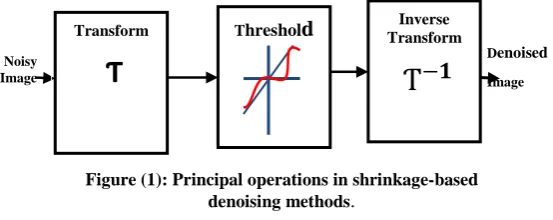
The main motivation of denoising in some transform domain is that in the transformed domain it may be possible to separate image and noise components. The basic principle behind most transform-domain denoising methods is shrinkage truncation (hard thresholding) or scaling (soft thresholding) of the transform coefficients to suppress the effects of noise, as shown in Figure (1). For such thresholding, the challenge is to develop a suitable coefficient mapping operation that does not sacrifice the details in the image. The final denoised image is obtained by performing an inverse transform on

the shrunk coefficients. This is done by first identifying photo metrically similar patches in the spatial domain. This group is then used to perform adaptive thresholding

in the shrinkage step. This allows them to process the entire group of patches simultaneously [16].

The codebook generation algorithm involves two important steps. The first step is the sparse coding step which involves finding the coefficients which can approximately represent the input features through a dictionary. The second step is dictionary updating which involves updating the base atoms of the dictionary through coordinate descent method with warm restarts.

5.

PCA CONCEPT FOR IMAGE

DENOISING

PCA is a classical decorrelation technique in statistical signal processing, it is fully de-correlates the original data set where converts a set of observations of possibly correlated variables into a set of values of uncorrelated variables called principal components. The number of principal components is less than or equal to the number of original variables. This transformation is defined in such a way that the first principal component has as high a variance as possible and each succeeding component in turn has the highest variance among the remaining components. The dimensionality of the data can then be reduced by selecting only the first few principal components [15]. So that the energy of the signal will concentrate on the small subset of PCA transformed dataset. The energy of random noise evenly spreads over the whole data set, so it easily to distinguish signal from random noise over PCA domain [4].

PCA is the way of identifying patterns in data, and expressing the data in such a way as to highlight their similarities and differences. The other main advantage of PCA is that once you have found these patterns in the data and you compress the data by reducing the number of dimensions without much loss of information. This technique used in image compression [4]. Generally speaking, the signal and noise can be better distinguished in the PCA domain. So the noise and trivial information can be removed.

Denote by 𝑧 = 𝑧1 𝑧2⋯ 𝑧𝑚 𝑇an m-component vector variable and denote by

𝑧

= 𝑧11 𝑧12

𝑧21 𝑧22

… …

… … ⋮

𝑧1𝑛

𝑧2𝑛

… 𝑧𝑚1 𝑧𝑚2 𝑧𝑚𝑛

(3) Figure (1): Principal operations in shrinkage-based

denoising methods.

Denoised Image Transform

Ƭ

Threshol

d

Ƭ

−𝟏

The sample matrix of 𝑧 𝑤𝑕𝑒𝑟𝑒 𝑧_𝑖𝑗, 𝑗 = 1,2, ⋯ , 𝑛., are the discrete samples of variable 𝑧𝑖, 𝑖 = 1,2, ⋯ 𝑚.. The ith

row of sample matrix, denoted by 𝑍𝑖

= 𝑧_𝑖1 _𝑧

𝑖2 ⋯ 𝑧𝑖𝑛 (4)

Is called the sample vector of 𝑧𝑖 . The mean value of 𝑍𝑖

is calculated as 𝜇𝑖

=1

𝑛 𝑧𝑖(𝑗)

𝑛

𝑗 =1

(5)

And then the sample vector 𝑍𝑖 is centralized as 𝑍 𝑖= 𝑍𝑖− 𝜇𝑖

= 𝑧 𝑖1 𝑧 𝑖2 ⋯ 𝑧 𝑖𝑛 (6)

where 𝑧 _𝑖𝑗 = 𝑧_𝑖𝑗 − 𝜇𝑖 . Accordingly, the centralized matrix of 𝑍 is

𝑍

= 𝑍 1𝑇 𝑍 2𝑇 ⋯ 𝑧 𝑚𝑇 𝑇 (7)

Finally, the co-variance matrix of the centralized dataset is calculated as

Ω

=1

𝑛𝑍𝑍 𝑇 (8) The goal of PCA is to find an orthonormal transformation matrix 𝑃 to decorrelate 𝑍 ,𝑌 = 𝑃𝑍 so that the co-variance matrix of 𝑌 is diagonal. Since the covariance matrix Ω is symmetrical, it can be written as: Ω

= 𝜙Λ𝜙𝑇 ₍₉₎

Where Φ= 𝜙1 𝜙2 ⋯ 𝜙𝑚 is the 𝑚𝑥𝑚 orthonormal eigenvector matrix and Λ= 𝑑𝑖𝑎𝑔{𝜆1, 𝜆2, ⋯ , 𝜆𝑚} is the diagonal eigenvalue matrix with 𝜆1> 𝜆2> ⋯ ≥ 𝜆𝑚. The terms

𝜙1 𝜙2 ⋯ 𝜙𝑚and 𝜆1, 𝜆2, ⋯ , 𝜆𝑚 are the eigenvectors

and eigenvalues of Ω. By setting 𝑃

=Φ𝑇 (10)

𝑍 can be decorrelated, 𝑌 = 𝑃𝑍 𝑎𝑛𝑑 Λ= 1 n 𝑌𝑌 𝑇 . From the point of view of image modeling, the PCA basis has the interesting property that, among all basis expansions, it minimizes the reconstruction error when the expansion is truncated to a smaller number of basis vectors. Thus, a class of high-dimensional images can be described by a low-dimensional model containing only a few principal components. Computationally, it can be advantageous to solve the eigenvalue problem by iterative methods which do not need to compute and store Ω directly. This is particularly useful when the size of Ω is large such that the memory complexity becomes prohibitive. PCA image models have been used, for instance, for image coding and texture segmentation.

6.

LPG-PCA

(THE

MAIN

LEARNING METHOD)

This paper propose to perform several PCAs on subsets of patches presenting less variability, for instance inside

small image regions patches. The advantage of this approach is that the resulting basis is not only adapted to the image but also to the region of the image containing the patch of interest.

PCA-based scheme was proposed for image denoising by using a moving window to calculate the local statistics, from which the local PCA transformation matrix was estimated. However, this scheme applies PCA directly to the noisy image without data selection and many noise residual and visual artifacts will appear in the denoised outputs. LPG-PCA models a pixel and its nearest neighbors as a vector variable. The training samples of this variable are selected by grouping the pixels with similar local spatial structures to the underlying one in the local window, whose training samples are selected from the local window by using block matching based LPG. The LPG algorithm guarantees that only the sample blocks with similar contents are used in the local statistics calculation for PCA transform estimation, so that the image local features can be well preserved after coefficient shrinkage in the PCA domain to remove the random noise [4]. With such an LPG procedure, the local statistics of the variables can be accurately computed so that the image edge structures can be well preserved after shrinkage in the PCA domain for noise removal.So that the Local Model from Sparse Representation: Similar to the patch-based methods mentioned tries to infer the HR image patch for each LR image patch from the input, from this local model [9].

The LPG-PCA enhancement procedure is iterated one more time to further improve the enhancement performance, and the noise level is adaptively adjusted in the next stage, the proposed LPG-PCA algorithm has two stages. The first stage yields an initial estimation of the image by removing most of the noise then the random noise is significantly reduced in the first stage; then the second stage will further refine the output of the first stage to more improve LPG-PCA is iterate more than two stages. The all stages have the same procedures except for the parameter of noise level. Since the noise is significantly reduced in the first stage, the LPG accuracy will be much improved in the next stage so that the final denoising result is visually much better. Hence the final enhancement result is also visually much better. The LPG-PCA enhance procedure is used to improve the image quality from first stage to second stage with edge preservation.

Compared with WT that uses a fixed basis function to decompose the image, the proposed LPG-PCA method is a spatially adaptive image representation so that it can better characterize the image local structures [5].

6.1.

Modeling of Spatially

edge structures, edge preservation is highly desired in image denoising. To this end, then model a pixel and its nearest neighbors as a vector variable and perform noise reduction on the vector instead of the single pixel.

Referring to Figure (2), for an underlying pixel to be denoised, we set a 𝑘𝑥𝑘 window centered on it and denote by 𝑧 = 𝑧1 𝑧2⋯ 𝑧𝑚 𝑇, 𝑚 = 𝑘2 the vector containing

all the components within the window. Since the observed image is noise corrupted, we denote by 𝑍𝑉=

𝑍 + 𝑣 ( 4.11)

The noisy vector of 𝑧, where 𝑧𝑣= 𝑧1𝑣 ⋯ ⋯ 𝑧𝑚𝑣 𝑇,𝑣 = 𝑣1 ⋯ ⋯ 𝑣𝑚 𝑇 and 𝑧𝑘𝑣 = 𝑧𝑘+ 𝑣𝑘, 𝑘 = 1,2, ⋯ , 𝑚 .To estimate 𝑧 from 𝑧𝑣 then view them as (noiseless and noisy) vector variables so that the statistical methods such as PCA can be used.

In order to remove the noise from 𝑍𝑣 by using PCA, then need a set of training samples of 𝑍𝑣 so that the

covariance matrix of 𝑍𝑣 and hence the PCA

transformation matrix can be calculated. For this purpose, we use a 𝑙𝑥𝑙 ( 𝑙 > k) training block centered on 𝑍𝑣 to find the training samples, as shown in (2). The

simplest way is to take the pixels in each possible 𝑘𝑥𝑘 block within the 𝑙𝑥𝑙 training block as the samples of noisy variable 𝑍𝑣. In this way, there are totally (𝑙 − 𝑘 +

1)2 _{training samples for each component 𝑧} 𝑘𝑣 𝑜𝑓 𝑍𝑣

However, there can be very different blocks from the given central 𝑘𝑥𝑘 block in the 𝑙𝑥𝑙 training window so that taking all the 𝑘𝑥𝑘 blocks as the training samples of 𝑍𝑣 will lead to inaccurate estimation of the covariance

matrix of 𝑍𝑣, which subsequently leads to inaccurate

estimation of the PCA transformation matrix and finally results in much noise residual. Therefore, selecting and grouping the training samples that similar to the central 𝑘𝑥𝑘 block is necessary before applying the PCA transform for denoising.

Grouping the training sample similar to the central 𝑘𝑥𝑘 block in the 𝑙𝑥𝑙 training window is indeed a classification problem and thus different grouping methods, such as block matching, correlation-based matching , K-means clustering, can be employed based on different criteria. Among them the block matching method may be the simplest yet very efficient one. There are totally (𝑙 − 𝑘 + 1)2 _{possible training blocks of 𝑍}

𝑣 in the 𝑙𝑥𝑙 training

window [17].

6.2.

Adaptive PCA Denoising

The algorithm (the PCA transform of LPG output image) is composed of the following steps [4]:

 Get some data.

 Subtract the mean.

 Calculate the covariance matrix.

 Calculate the eigenvectors and eigenvalues of the covariance matrix.

 Choosing components and forming a feature vector.

 Deriving the new data set.

 Apply the soft thresholding of PCA output image.

 Take inverse PCA.

6.3.

Refinement The Result

Most of the noise will be removed by using the denoising procedures described in the previous Sections. However, there is still much visually unpleasant noise residual in the denoised image. There are mainly two reasons for the noise residual. First, because of the strong noise in the original dataset 𝑍𝑣 , the covariance matrix is much noise

corrupted, which leads to estimation bias of the PCA transformation matrix and hence deteriorates the denoising performance; second, the strong noise in the original dataset will also lead to LPG errors, which consequently results in estimation bias of the covariance matrix. Therefore, it is necessary to further process the denoising output for a better noise reduction. Since the noise has been much removed in the first round of LPG-PCA denoising, the LPG accuracy and the estimation of covariance matrix can be much improved with the denoised image. Thus we can implement the LPG-PCA denoising procedure for the next rounds to enhance the denoising results [5].

7.

EXPERIMENTAL RESULTS

Experimental results on test images demonstrate that the LPG-PCA method achieves very competitive denoising performance, especially in image fine structure preservation. The LPG-PCA denoising algorithm uses PCA to adaptively compute the local image decomposition transform so that it can better represent the image local structure. In addition, the LPG operation is employed to ensure that only the right samples are involved in PCA training. This method performed various experiments on simulated and real data to be validated.

In the implementation of LPG-PCA denoising, actually the complete 𝑘𝑥𝑘 block centered on the given pixel will be denoised. Therefore, the finally restored value at a pixel can be set as the average of all the estimates obtained by all windows containing the pixel. Some images (Parrot and Lena image) are trained, and then zero mean white Gaussian noise of different standard deviations (σ) artificially added to the original image to produce noisy images. Here the different methods evaluate and compare by using two measures: PSNR and MSE.

To verify from the improvement of the noise removal in the second stage of the PLG-PCA method. Table (1) lists the PSNR and MSE measures of the first stage and second stage denoising outputs on the test Parrot image set. From the table can noted that the second stage can improve 0.1–1.5dB the PSNR values for different images under different noise level (σ is from5 to 70).

The LXL training block The pixel to be denoised

The KXK variable block

Table (1): the MSE and PSNR values for Parrot image from LPG-PCA method (first stage and second stage) for

different cases of standard deviation (σ).

IMAGE PARROT IMAGE σ MSE for

noisy

MSE for LPG 1st

MSE for LPG

2nd

PSNR for noisy

PSNR for LPG

1st

PSNR for LPG

2nd 5 24.872 64.209 84.578 34.174 30.055 28.858 10 97.730 65.789 83.066 28.231 29.949 28.937 15 214.904 70.406 81.622 24.808 29.655 29.013 20 373.576 89.426 88.036 22.407 28.616 28.684 25 571.212 145.832 130.139 20.563 26.492 26.987 30 806.609 256.921 231.164 19.064 24.033 24.492 35 1077.212 429.49 393.112 17.808 21.801 22.186 40 1380.783 657.353 610.397 16.729 19.953 20.275 50 2066.818 1233.659 1168.344 14.978 17.219 17.455 60 2832.064 1916.824 1836.480 13.609 15.305 15.491 70 3639.931 2656.77 2564.344 12.519 13.887 14.041

Table (2) a same as Table (1) lists the PSNR and MSE measures of the first stage and second stage denoising outputs on the test Lena image set. Also can noted that the second stage can improve 0.1–1 dB the PSNR values for different images under different noise level (σ is from5 to 70).

here a controlled simulated experiment is set up by adding white Gaussian noise with standard deviation (σ =30) to the Parrot and Lena image (128×128) shown in Figure (3(a) )and Figure (4(a)) , while the resulting noisy image is shown in Figure. (3(b)) and Figure (4(b)). The noisy image is then denoised by the LPG-PCA of the first stage, result of which is shown in Figure (3(c)) and

Figure (4(c)). Then the noisy image is denoised by the LPG-PCA of the second stage, result of which is shown in Figure (3(d)) and Figure (4(d)).

(a) original (b) noisy (MSE=806.653, PSNR=19.0639)

(c) 1st LPG-PCA (MSE= 256. 92, PSNR=24.03)

(d) second LPG-PCA (MSE =231.16, PSNR=24.49) Figure (3): the MSE and PSNR for Parrot image vary with first and second stage for LPG-PCA for additive white Gaussian noise of standard deviation (σ=30)

For the parrot image shown in Figure (3), the method was found to give the best results when the image (with σ=30) was denoised by two type of LPG-PCA and noted the different on MSE and PSNR as metric. According to Figure (3) PSNR increase by 5db more than noisy image after applying LPG-PCA first stage and by 5.5db after applying LPG-PCA second stage.

For the Lena image shown in Figure (4), the method was found to give the best results when the image (with σ=30) was denoised by two type of LPG-PCA and noted the different on MSE and PSNR as metric. According to Figure (4) PSNR increase by 5db more than noisy image after applying LPG-PCA first stage and by 5.5db after applying LPG-PCA second stage.

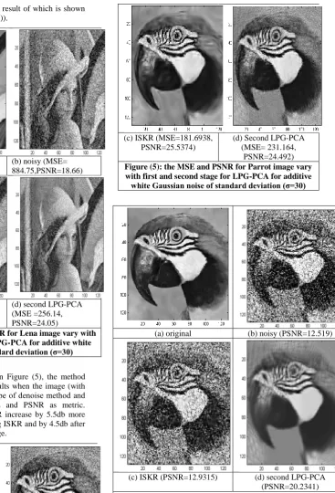
Then a compare between the different methods on denoising is made. Figure (5) and Figure (6); list the PSNR and MSE results by different methods (ISKR and LPG-PCA) on the Parrot image at different standard deviation (σ). A controlled simulated experiment is set up by adding white Gaussian noise with standard deviation (σ =30, 70) to the Parrot image (128×128) shown in Figure (5(a)) and Figure (6(a)), while the resulting noisy image is shown in Figure. (5(b)) and Figure (6(b)). The noisy image is then denoised by the ISKR, result of which is shown in Figure (5(c)) and Figure (6(c)). Then the noisy image is denoised by the Table (2): the MSE and PSNR values for Lena image from

LPG-PCA method (first stage and second stage) for different cases of standard deviation (σ). IMAGE LENA IMAGE

σ MSE

for noisy

MSE for LPG

1st

MSE for LPG

2nd

PSNR for noisy

PSNR for LPG

1st PS NR

for LP

G 2nd

5 25.155 60.851 79.398 34.125 30.288 29.1 33 10 100.621 60.662 76.396 28.104 30.302 29.3

00 15 226.361 62.402 72.205 24.583 30.179 29.5

45 20 401.213 82.012 77.272 22.097 28.992 29.2

51 25 621.743 151.099 131.162 20.195 26.338 26.9

53 30 884.754 288.472 256.140 18.663 23.529 24.0

46 35 1185.57 494.613 448.847 17.392 21.188 21.6

09 40 1517.67 756.34 697.876 16.319 19.344 19.6

93 50 2258.70 1388.49 1310.60 14.592 16.705 16.9

56 60 3064.29 2106.70 2014.41 13.268 14.895 15.0

89 70 3897.69 2864.14 2760.31 12.223 13.561 13.7

LPG-PCA of the second stage, result of which is shown in Figure (5(d)) and Figure (6(d)).

(a) original (b) noisy (MSE= 884.75,PSNR=18.66)

(c) 1st LPG-PCA (MSE=288. 47, PSNR=23.53)

(d) second LPG-PCA (MSE =256.14, PSNR=24.05)

Figure (4): the MSE and PSNR for Lena image vary with first and second stage for LPG-PCA for additive white

Gaussian noise of standard deviation (σ=30)

For the Parrot image shown in Figure (5), the method was found to give the best results when the image (with σ=30) was denoised by two type of denoise method and noted the different on MSE and PSNR as metric. According to Figure (5) PSNR increase by 5.5db more than noisy image after applying ISKR and by 4.5db after applying LPG-PCA second stage.

(a) original (b) noisy (MSE=806.65, PSNR=19.064)

(c) ISKR (MSE=181.6938, PSNR=25.5374)

(d) Second LPG-PCA (MSE= 231.164,

PSNR=24.492) Figure (5): the MSE and PSNR for Parrot image vary with first and second stage for LPG-PCA for additive white Gaussian noise of standard deviation (σ=30)

(a) original (b) noisy (PSNR=12.519)

(c) ISKR (PSNR=12.9315) (d) second LPG-PCA (PSNR=20.2341) Figure (6): the MSE and PSNR for Parrot image vary with first

and second stage for LPG-PCA for additive white Gaussian noise of standard deviation (σ=70)

Furthermore try to make some modify on local window before perform PCA transform on it this modify include, change number of iteration according to the amount of noise on image additionally using the benefited of (SKR) to prepare the noisy image before apply LPG-PCA. While KR is a well studied method in statistics and signal processing, KR is identified as a nonparametric approach that requires minimal assumptions, and hence the framework is one of the appropriate approaches to the regression problem.

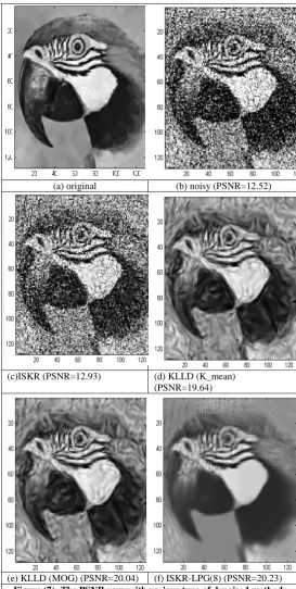
We then compare the different methods on denoising. Figure (7), list the PSNR results by different methods (ISKR, KLLD (K_mean), KLLD (MOG) and ISKR-LPG on the Parrot image at standard deviation (σ=70). A controlled simulated experiment is set up by adding white Gaussian noise with standard deviation (σ = 70) to the Parrot image (128×128) shown in Figure (7(a)), while the resulting noisy image is shown in Figure. (7(b)) and. The noisy image is then denoised by the ISKR, result of which is shown in Figure (7(c)). Then the noisy image is denoised by the KLLD (K_mean), result of which is shown in Figure (7(d)). Then the noisy image is denoised by the KLLD (MOG), result of which is shown in Figure (7(e)). Then the noisy image is denoised by the ISKR-LPG, result of which is shown in Figure (7(f)). For the Parrot image shown in Figure (7), the method was found to give the best results when the image (with σ=70) was denoised by four type of denoise method and noted the different on PSNR as metric. According to Figure (7) PSNR increase by .5db more than noisy image after applying ISKR and by 7db after applying KLLD (K_mean) and by 7.5b after applying KLLD (MOG) and by 7.8db after applying ISKR-LPG by eight times of iteration.

8.

CONCLUSION

This paper presents a SR method based on sparse representation, which builds sparse association between image feature patches, and at the same time carry on matching and optimization. Compared with other sparse coding method, sparse representation is more compressible and efficient, and needs fewer examples for the same quality. Comparison with other learning-based super-resolution method shows that our method superior in quality and computation. However, there are some possibilities for future improvement. Through the proposed method used PCA. To preserve the local image structures when denoising, then a pixel and its nearest neighbors are modeled as a vector variable, and the denoising of the pixel was converted into the estimation of the variable from its noisy observations. The PCA transformation matrix was adaptively trained from the local window of the image. The block matching based LPG was used for such a purpose and it guarantees that only the similar sample blocks to the given one are used in the PCA transform matrix estimation. LPG- PCA denoising procedure was iterated one more time to improve the denoising performance. Additionally used the kernel regression framework as an efficient tool in image processing, and found its relation with popular existing denoising and interpolation techniques. Experimental results demonstrated that LPG-PCA can effectively preserve the image fine structures while smoothing noise.

(a) original (b) noisy (PSNR=12.52)

(c)ISKR (PSNR=12.93) (d) KLLD (K_mean) (PSNR=19.64)

(e) KLLD (MOG) (PSNR=20.04) (f) ISKR-LPG(8) (PSNR=20.23) Figure (7): The PSNR vary with various type of denoised methods

for additive white Gaussian noise of standard deviation (σ=70)

9.

REFERENCES

[1] Naveen Kulkarni, „ Compressive Sensing for Computer Vision and Image Processing‟, Approved May 2011.

[2] Jianchao Yang, Student Member, IEEE, John Wright, Member, IEEE, Thomas S. Huang, Fellow, IEEE, and Yi Ma, Senior Member, IEEE, ‘Image Super-Resolution Via Sparse Representation’ ,

IEEE TRANSACTIONS ON IMAGE

PROCESSING, VOL. 19, NO. 11, NOVEMBER 2010.

[3] H. Lee, A. Battle , R. Raina , A.Y. Ng, Efficient sparse coding algorithms, NIPS, 2007.

[4] Vikas D Patil ,„PCA Based Image Enhancement in Wavelet Domain‟, International Journal of Engineering Trends and Technology- Volume3Issue1- 2012.

[5] Lei Zhang, „Two-stage image denoising by principal component analysis with local pixel grouping‟, Pattern Recognition 43 (2010) 1531– 1549.

[6] M. Aharon, M. Elad, A.M. Bruckstein, The K-SVD: an algorithm for designing of overcomplete dictionaries for sparse representation, IEEE Transaction on Signal Processing 54 (11) (2006) 4311–4322.

[7] M. Elad, M. Aharon, Image denoising via sparse and redundant representations over learned dictionaries, IEEE Transaction on Image Processing 15 (12) (2006) 3736–3745.

[8] A. Foi, V. Katkovnik, K. Egiazarian, Pointwise shape-adaptive DCT for high- quality denoising and deblocking of grayscale and color images, IEEE Transaction on Image Processing 16 (5) (2007).

[9] Jianchao Yang, Student Member, IEEE, John Wright, Member, IEEE, Thomas S. Huang, Fellow, IEEE, and Yi Ma, Senior Member, IEEE, ‘Image Super-Resolution Via Sparse Representation’ ,

IEEE TRANSACTIONS ON IMAGE

PROCESSING, VOL. 19, NO. 11, NOVEMBER 2010.

[10] L. C. Yang, L. Wright, T. S. Huang, and Y. Ma, "Image superresolution as sparse representation of raw image patches," Computer Vision and Pattern Recognition (CVPR 2008). IEEE Conference on. 2008.

[11] Charles-Alban Deledalle, „Image denoising with patch based PCA: local versus global‟, c 2011. [12] E. J. Candes, “Compressive Sampling,” in Proc. Int.

Congr. Mathetmaticians,2006, vol. 3, pp. 1433– 1452.

[13] D. L. Donoho, “Compressed sensing,” IEEE Trans. Inf. Theory, vol.52, no. 4, pp. 1289–1306, Apr. 2006.

[14] D. Glasner, S. Bagon, and M. Irani. Super-resolution from a single image. In ICCV, 2009. [15] Kaustubh Anil Patwardhan, A FEATURE-BASED

ALGORITHM FOR SPIKE SORTING

INVOLVING INTELLIGENT FEATURE-WEIGHTING MECHANISM, July 2011.

[16] W. T. Freeman, E. C, Pasztor, and O. T. Carmichael. "Learning Low Level Vision,", International Journal of Computer Vision, Vol. 40, 2000, pp. 25-47.