Which Model Performs Better While Forecasting Stock Market Volatility? Answer for Dhaka Stock Exchange (DSE)

(1)

ISSN Print: 2162-2078

DOI: 10.4236/tel.2018.814199 Oct. 26, 2018 3203 Theoretical Economics Letters

Which Model Performs Better While

Forecasting Stock Market Volatility?

Answer for Dhaka Stock Exchange (DSE)

S. M. Abdullah

1

_{, Mohammod Akbar Kabir}

1

_{, Kawsar Jahan}

2

_{, Salina Siddiqua}

3

1_{Department of Economics, University of Dhaka,}_{Dhaka, Bangladesh}

2_{Department of Accounting & Information Systems, University of Dhaka, Dhaka, Bangladesh} 3_{Department of Development Studies, University of Dhaka, Dhaka, Bangladesh}

Abstract

An efficient and well behaved capital market can be regarded as a prerequisite for the sustainable financial development for an economy. For making the stock market efficient and reducing uncertainty, volatility measure is neces-sary for the policy makers. The main objective of this paper is to examine rel-ative ability of various models to forecast future volatility and to devise ap-propriate volatility model for capturing variability in stock returns of Dhaka

Stock Exchange (DSE). By exploiting daily data spanning from 27th

Novem-ber, 2001 to 31st_{July, 2013, it was found that, from volatility persistency}

pers-pective MA(2) − GARCH(2, 1) is better due to both in sample and out of sample accuracy. In contrast, from capturing asymmetric effect perspective MA(2) − EGARCH(1, 3) is better. Thus, there was no clear winner and hence the decision should depend on the purpose of the concerned people.

Keywords

Stock Market, Volatility Forecasting, GARCH, EGARCH, Mean Equation

1. Introduction

Stock Market volatility is the variability in stock prices during a period which is perceived as a measure of risk by investors. It may affect business investments,

financial market performance and economic performance directly [1] [2] [3].

Volatility of stock prices reflects uncertainty in the market. A rise in stock mar-ket volatility can often be interpreted as a rise in equity and thus a shift of funds to less risky assets; this move has been known to lead to a rise in the cost of

How to cite this paper: Abdullah, S.M., Kabir, M.A., Jahan, K. and Siddiqua, S. (2018) Which Model Performs Better While Forecasting Stock Market Volatility? Answer for Dhaka Stock Exchange (DSE). Theoretical Economics Letters, 8, 3203-3222.

https://doi.org/10.4236/tel.2018.814199

Received: September 25, 2018 Accepted: October 23, 2018 Published: October 26, 2018

http://creativecommons.org/licenses/by/4.0/

(2)

DOI: 10.4236/tel.2018.814199 3204 Theoretical Economics Letters

funds to firms [1]. The understanding of stock market volatility could be useful

in the determination of the cost of capital and in the evaluation of asset alloca-tion decision. Policy makers may rely on estimates of market volatility as an in-dicator of the vulnerability of financial markets [4][5]. Thus, the specification of appropriate volatility model for capturing variability in stock returns has a sig-nificant policy relevance to economic decision makers. Moreover, the ability to model and forecast volatility of asset returns is vital for investors in decision making about risk management and portfolio adjustments.

Like other developing countries in Bangladesh stock market is an emerging market but has been experiencing inefficiency from its inception. To make the market efficient and reduce uncertainty, volatility measure is necessary for the policy makers. The main objective of this paper is to examine relative ability of various models to forecast future volatility and to devise appropriate volatility model for capturing variability in stock returns of Dhaka Stock Exchange (DSE).

On this background already an enormous amount of effort has been made from the researchers to model the variance dynamics of stock market return and

its different characteristics in Bangladesh [6]-[15]. Some of them have given

ef-fort to find only the volatility persistency property of the stock return, some tried to model only the risk return relationship while some other tried to forecast the volatility only. All the exercises tried to address the issue applying Genera-lized Autoregressive Conditional Heteroscedasticity (GARCH) family models

developed by Bollerslev [16]. However, a few of papers have actually tried to

fig-ure out the best performing model for capturing the in-sample variance dynam-ics and out-of-sample variance forecasting. Also, identification of mean equation was either completely ignored or improperly identified and post estimation di-agnostic checking was also improper resulting in some findings which could re-main as questionable. The current study first aimed to develop appropriate mean equation and model the variance dynamics in stock return using number of li-near and non-lili-near GARCH family models. Secondly it made an effort to select an appropriate in sample variance model while capturing its different feature and also tried to find out the best one while out of sample variance forecasting is the purpose.

The rest of the article is organized as follows: Section 2 provides an overview of existing literature, Section 3 discusses about data, variable construction and model specification and Section 4 contains the estimation results and findings. Finally, Section 5 concludes.

2. Literature Review

Several researchers have examined the volatility of stock returns of Dhaka Stock Exchange (DSE). They considered different models for different time period and

sample size and found contradictory results in some cases. Rayhan et al. [8]

(3)

random walk. The study also revealed that monthly DSE returns follow Genera-lized Autoregressive conditional Heteroskedasticity (GARCH) properties.

Nev-ertheless Uddin et al. [15] while testing the efficient market hypothesis in pricing

securities and the relationship between stock returns and conditional volatility argued that the stocks in DSE follow a random walk. Therefore the market might meet the criterion of weak form efficiency. The results of GARCH (p, q) model indicate the tendency for returns to exhibit volatility clustering.

Earlier Huq et al. [11] considered daily stock exchange data (general index)

from December 06, 2010 to March 12, 2013, for building time series modeling and forecast. They used both symmetric and asymmetric models and found that the model ARMA(1, 1) with GARCH(1, 1) and GARCH(2, 1) are more appro-priate model for the general index of Dhaka Stock Exchange (DSE) for the said

study period. Aziz & Uddin [13] also estimated volatility in the DSE general

in-dex returns by GARCH(1, 1) models and found that the volatility is present in the stock market in Bangladesh which is decreasing over time. The

appropriate-ness of GARCH(1, 1) model has also been endorsed by Miah & Rahman [14]

who have employed Dhaka Stock Exchange (DSE) returns of four selected com-panies, namely BEICL, BPL, PBL and ABBL for the period January 2000 to

No-vember 2014. On a different note Basher et al. [7] empirically investigated the

time-varying risk return relationship within a GARCH-type framework and the impact of institutional factors like circuit breaker on volatility for the stock market of Bangladesh. The results showed a significant relationship between conditional volatility and stock returns, but the risk-return parameter is found to be sensitive to choice of samples and frequencies of data. While lock-in did not have any overall impact on stock volatility, the imposition of a circuit breaker has contributed significantly to the volatility of realized returns.

With a view to capture the asymmetric effect during 90s Chowdhury [6]

ana-lyzed the time series behaviour of Dhaka Stock Exchange Composite Index re-turns using the EGARCH-M model for the sample period December 1, 1988 to May 31, 1994, totaling 1519 observations. He concluded that there is asymmetry in the volatility of stock index return and unlike in the developed stock markets, positive return shocks in Dhaka stock market lead to higher increases in condi-tional volatility. In-sample and out-of-sample forecasting accuracy has been

considered by Rahman et al. [9] with the GARCH, EGARCH and APARCH

models in case of Dhaka Stock Exchange (DSE) from the period January 02,

1999 to December 29, 2005. Later on Alam et al. [12] investigated the use of

(4)

all models except GARCH and TARCH models are regarded as the best model jointly for DSE20 index returns series, while for DSE general index returns

se-ries, no model is nominated as the best model individually. Islam et al. [10]

ex-amined the relative ability of various linear and nonlinear models to forecast daily stock indexes of future volatility of Dhaka Stock Exchange (DSE) index DSE-20 and found that linear moving average model outperforms other linear and nonlinear models.

It is widely accepted that while modeling the variance the mean equation is of vital importance. As failure of appropriate model detection for mean might re-sult in less efficiency of parameters used in variance model due to potential presence of autocorrelation. This issue has largely been ignored in the stock market volatility literature in Bangladesh. Thus, the current study would at first optimize the mean equation while quest for modeling the variance dynamics in stock return. The main contribution here would be to set up appropriate volatil-ity model for efficiently capturing variance dynamics in stock returns of Dhaka Stock Exchange (DSE).

3. Methodological Framework

3.1. Data and Variable Construction

This paper has exploited the daily data on general stock price index of DSE

spanning from 27th_{November, 2001 to 31}st_{July, 2013}1_{. Although there are}

regu-lar fluctuations in the movement of stock price index, generally they do contain the unit root property and hence can be characterized as nonstationary in na-ture. Thus, we have used logarithmic transformation to convert the data into stock market return which would have greater possibility to be stationary and appropriate for analysis. We have used the following formula to measure the re-turn:

( )

1

ln ln

t t

r = P − P−

Here, rt stands for stock market return at day t, Pt and Pt−1 stands for general stock price index at day t and day before t. EViews 9 has been used as the statistical software for performing quantitative exercise.

3.2. Model Specification

The perfect modeling of conditional mean can be considered as a prerequisite of correct model specification of conditional variance of stock market return. Along with independent variables researchers of volatility modeling usually augment the conditional mean model either with Autoregressive (AR) or with Moving Average (MA) or even with a mixture of these two (Autoregressive

Moving Average, ARMA) process [17]. In our case to serve the purpose we have

used both AR (p) and MA (q) specification with sufficient lags in the following way:

(5)

DOI: 10.4236/tel.2018.814199 3207 Theoretical Economics Letters 1

p

t i t i t i

r µ θr− ε

=

= +

∑

+

1

q

t i t i t i

r µ φ ε₋ ε

=

= +

∑

+

where,

µ

_{is the constant term,}θ θ₁, , ,₂ θp and φ φ1, , ,2 φq are the lagged

coefficients and εt is a white noise process. For modeling the volatility in stock

market return using the above two different types of mean equation, the variance equation is specified following family of GARCH models namely, Standard GARCH, APARCH, EGARCH and IGRACH models. GARCH models

devel-oped by Bollerslev [16] are superior to their earlier versions called ARCH

devel-oped by Engle [18] as they ensure improvement in efficiency due to required

es-timation of lower number of parameters. However, consider the following gen-eral specification of the variance model:

t h vt t

ε

=

Here, v iidt ∼

( )

0,1 , and specification of ht will determine different varieties

of GARCH family models while each of which will serve specific purpose. For analyzing the different feature of stock market return by modeling its volatility we have estimated the following models:

(

)

2

1 1

GARCH , : t q i t i p j t j

i i

p q h η α ε− β h−

= =

= +

∑

+

∑

(

)

(

)

( )

1 1

APARCH , : _t q _i _{t i} _{i t i} p _j _{t j}

i j

p q h η α ε− γ ε− δ β h− δ

= =

= +

∑

− +

∑

(

)

( )

1 1

EGARCH , : ln q t i t i p ln

t i i j t j

i _{t i} _{t i} j

p q h h

h h

ε ε

η α − λ − β

− = ₋ ₋ =     = + + +    

∑

(

)

2

1 1 1 1

IGARCH , : t q i t i p j t j, where, q i p j 1

i j i j

p q h α ε− β h− α β

= = = =

=

∑

+

∑

+

∑

=

Here, in GARCH(p, q) model, p and q denotes the lag order of GARCH and ARCH terms respectively. In order to have well behaved variance restrictions on

the parameters needed to be imposed, for instance, η>0,αi≥0 and βj ≥0.

The volatility persistence will be measured by summing up the ARCH and

GARCH coefficients

(

q₁ p₁

)

i i j i=α +

∑

=β

∑

which is expected to be less than unity

to have a stationary residual and nonnegative variance.

APARCH model developed by Ding, Granger & Engel [19] is used to capture

the nonlinear variance equation. Similarly as before p and q denotes the lag

or-der of GARCH and ARCH terms with βj and αi as their coefficients

respec-tively. The parameter

δ

_{denotes the power parameter which is expected to be}

strictly positive. In particular the parameter of interest in such models is γi; the

significance of which ensures the presence of leverage effect. The γ parameter

addresses the leverage effect of order up to k where,

γ

_i ≤ ∀ =1 i 1,2,_k_and

0

i i k

γ = ∀ > _and k q≤ _.

(6)

de-DOI: 10.4236/tel.2018.814199 3208 Theoretical Economics Letters

veloped by Nelson [20]. In the above EGARCH specification βj is the

para-meter measuring persistence in volatility, αi is the parameter measuring

leve-rage effect and hence named as “asymmetry parameter”, finally λi is the

para-meter measuring magnitude of the shocks and thus named as “size parapara-meter”. Since EGARCH expressed conditional variance as an exponential function un-like the earlier models it is not subject to nonnegativity restrictions.

Engle & Bollerslev [16] have pioneered the IGARCH model for modeling the

variance which is nonstationary in nature. Thus, IGARCH can be characterized as non stationary GARCH model. In the above IGARCH(p, q) process the sum of ARCH and GARCH coefficients would be equal to unity and thus individually they would contain a value less than unit.

To choose among the conditional heteroscedasticity models we have com-pared their out of sample volatility forecasting performance. In particular dif-ferent models with several specifications have been compared in terms of Root Mean Square Error (RMSE), Mean Absolute Error (MAE), Mean Absolute Per-cent Error (MAPE) and Theil Inequality (TI) for identifying the most appropri-ate one with the current data.

4. Estimation Results and Findings

4.1. In Sample Estimation Results

As discussed in Section 3 it is imperative to identify the conditional mean model appropriately for modeling the volatility in concerned variable. Therefore, selec-tion of estimaselec-tion method of condiselec-tional mean model for stock return series is

of vital importance. Figure A1 (Appendix) presents the time series graph of

DSE General Index and their corresponding stock return series and Table A1

(Appendix) contains the summary statistics of the DSE General Index. It is quite evident from the figure that behavior of DSE General Index would be non sta-tionary as the possibility of mean reversion would be very low. In contrast, since the mean reversion would possibly be quite frequent in stock return series it might exhibit the stationary behavior. To shed light on the perception we have from graphical analysis of this two series, statistical tests have been performed.

Table A2 (Appendix) contains the test results for the unit root property of the stock return. We have used two different tests to diagnose the property;

Aug-mented Dickey Fuller (ADF) [21] and Kwiatkowski-Philips-Schmidt-Shin

(KPSS) [22]. The former one test the null of non-stationarity of the series while

the later considers the null as the stationary one. Both the tests have been per-formed with two different specifications; one with drift and the other with drift and trend. As the results show we can reject the null of non-stationarity of stock return in both test specifications under ADF at 1 percent level. On the other hand while performing KPSS test the null of stationarity of the variable was not possible to reject as the calculated value of test statistic was found to be lower

than its corresponding 1 per cent critical value (Appendix: Table A2). Thus it

(7)

use OLS directly as estimation method for the conditional mean models.

The conditional mean model for stock return has been developed with two

specifications one with AR terms and the other with MA terms. Table 1 contains

the estimation results. It can be observed that to capture the dynamics in stock return in AR specification an AR(2) and in MA specification an MA(2) model was estimated. The conditional mean models have not been augmented further

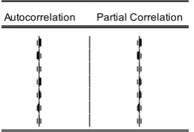
with AR or MA terms as they were not significant (Figure A2, Appendix).

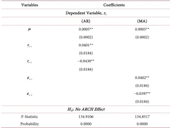
Ta-ble 1 also contains the result for testing the existence of ARCH effect. It is re-vealed that in both AR(2) and MA(2) specification the test statistic for the null saying “there is no ARCH effect” can be convincingly rejected with statistical evidence. Thus, the test is statistically significant implying that stock market re-turn in Bangladesh is conditionally heteroscedastic. So, modeling the volatility clustering can be of important as it would help to analyze the inherent characte-ristics of the market in a more applied manner. The existence of volatility clus-tering in stock return series has also been found evident from the residual plot in

Figure A3 (Appendix).

Since ARCH effect was present we have tried to model the volatility clustering using GARCH family models and explain the characteristics of the market while capturing its variance dynamics. To begin with we have estimated standard GARCH model both with AR(2) and MA(2) conditional mean specification.

Ta-ble A3 (Appendix) and Table 2 contains the estimation results. As the results

[image:7.595.204.538.448.699.2]

show in AR-GARCH specification the AR(1) coefficient is significant in all the models while the AR(2) coefficient was insignificant. Almost in all specifications

Table 1. Estimation of different conditional mean models and testing for ARCH effect.

Variables Coefficients

Dependent Variable, rt

(AR) (MA)

µ _0.0005** _0.0005**

(0.0002) (0.0002)

1

−

t

r 0.0401**

(0.0184)

2

−

t

r −0.0430**

(0.0184)

1

−

t

ε 0.0402**

(0.0184)

2

−

t

ε −0.0397**

(0.0184) HO: No ARCH Effect

F-Statistic 134.9106 134.8517

Probability 0.0000 0.0000

(8)

[image:8.595.210.537.89.585.2]

Table 2. Estimation results of GARCH models with MA mean specification.

Coefficients GARCH

(1, 1) (1, 2) (1, 3) (1, 4) (2, 1)

µ _0.0014** _0.0034* _0.0033* _0.0013** _0.0013**

(0.0006) (0.0003) (0.0003) (0.0006) (0.0005)

1

φ 0.0862*** 0.0629** 0.0657*** 0.0987*** 0.1096** (0.0469) (0.0312) (0.0363) (0.0523) (0.0461)

2

φ −0.0384 −0.0435** −0.0197 −0.0322 −0.0389 (0.0323) (0.0215) (0.0213) (0.0422) (0.0366)

η _1.25E−05 _6.11E−05* _3.49E−05* _5.38E−06* _1.29E−05**

(7.73E−06) (2.58E−06) (2.88E−06) (1.86E−06) (5.91E−06)

1

α 0.3465* 0.3195* 0.3365* 0.2770* 0.1839** (0.1104) (0.0490) (0.0332) (0.0911) (0.0850)

2

α _0.4115

(0.3785)

1

β 0.6684* 0.7351* 0.9718* 1.4214* 0.5159* (0.0789) (0.1755) (0.1252) (0.0963) (0.1580)

2

β −0.2042*** −0.4266* −1.1294* (0.1121) (0.0965) (0.1612)

3

β _0.0768* _0.5980*

(0.0199) (0.1286)

4

β −0.1167**

(0.0496)

Q1 (5) 33.554* 31.074* 32.508* 36.777* 32.264* Q1 (10) 39.896* 37.997* 38.392* 44.698* 40.258* Q2 (5) 0.1161 0.1643 0.0911 0.1289 0.2274 Q2 (10) 0.3068 1.1046 0.1850 0.4465 0.5983 Log Likelihood 8700.438 8530.647 8600.336 8740.959 8746.996

F Stat. 0.0512 6.42E−05 0.0252 0.0528 0.0132 Prob. 0.8208 0.9936 0.8739 0.8093 0.9084 Note: Robust Standard Errors are in Parenthesis. *** indicates significant at 10 per cent level, ** indicates significant at 5 per cent level and * indicates that at 1 per cent level.

the constant,

η

and the ARCH coefficient,

α

is positive and significant.

However, though the GARCH coefficients denoted by

β

has been found to be

(9)

coeffi-DOI: 10.4236/tel.2018.814199 3211 Theoretical Economics Letters

cient was found to be positive significant while the second ARCH coefficient was insignificant. The sum of ARCH and GARCH coefficients remained less than unity with a positive significant constant. Thus it satisfies all the restrictions and might be a potential model.

The residuals of the GARCH models are needed to be white noise. Thus, a di-agnostic test in the form of Ljung-Box Q test has been performed under the null

hypothesis, (H0: No Serial Correlation in the Error Term). We calculate

Q-Statistics for the standardized residuals (Q1) and for their squared values (Q2). It can be seen that all Q1-Statistics are significant at 1 per cent level while the Q2-Statistics were not. Therefore autocorrelation was found when we test based on level residuals and that was absent when test based on squared resi-duals. Nevertheless as F-statistic turn out to be insignificant for all models, it can be argued that none of them have ARCH effect. As the post estimation diagnos-tic results was found to be same for all but AR(2) − GARCH(2, 1) is the one which satisfies the restrictions, it can be treated as the appropriate one. Here the models were not augmented further as the coefficients were not found to be significant.

While the variance modeling was performed with MA mean specification the findings turn out to be almost same. However, MA(2) − GARCH(2, 1) specifica-tion has been observed to follow all the required restricspecifica-tions with the similar post diagnostic properties as AR(2) − GARCH(2, 1). It is evident from the find-ings that among these two the former one have higher (8746.99) log likelihood than the later (8739.313), also the information criteria for the former one (SIC = −5.9597) is found to be lower than the later (SIC = −5.9585). Therefore, model-ing volatility of stock return with MA mean specification has been revealed to be more appropriate than its AR counterpart.

For introducing nonlinearity in the variance equation and analyzing the asymmetric feature of volatility in the stock market return we have estimated APACRH model. As MA specification was found to provide more appropriate

result, for mean equation MA(2) specification was used. Table A4 (Appendix)

contains the estimation results. In particular we have estimated MA(2) − APARCH(1, 1) model. Further augmentation has not been done as the

coeffi-cients were not significant. As the results show the coefficoeffi-cients α and β have

found to be statistically significant with a positive sign. The power parameter δ is also positive and significant. Thus the model satisfies all the restrictions. The significance and sign of the coefficient, γ determines the leverage effect. Here, as the coefficient was not found to be significant, MA(2) − APARCH(1, 1) specifi-cation reveals that there is no leverage effect in stock market return in Bangla-desh. Therefore, possibly there is no asymmetric volatility effect in the stock market return. The post estimation diagnostic results of this model show that there is no ARCH effect and there is no autocorrelation in the squared residuals.

(10)

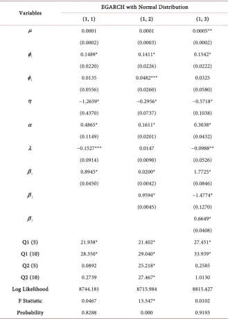
capturing the asymmetric volatility effect. Also, along with “asymmetry parame-ter” it estimates another parameter called “size parameparame-ter” measuring the size of shocks. Thus in contrast to APARCH, EGARCH can measure the existence of

leverage effect as well as the magnitude of shock. Table 3 contains the

estima-tion results. In particular we have estimated EGARCH(1, 1), EGARCH(1, 2) and EGARCH(1, 3) for variance equation while modeling the conditional mean with MA(2) specification. As the coefficients have not been found to be significant we

didn’t augment the model further. Here β’s are the persistence parameters, 𝛼𝛼is

the parameter and γ is the size parameter. It can be observed that in all specifica-tions the persistence parameters and the asymmetry parameters are statistically significant. In particular, the asymmetry parameter was statistically significant with a positive sign. Thus there exists significant leverage effect and the effect of “good news” and “bad news” in the stock market return does not necessarily cause symmetric variation in the stock return. As the leverage coefficient is found to have a positive sign, it can be argued that positive shocks (good news) increases volatility more than the negative shocks (bad news) of the same mag-nitude.

The results on diagnostic indicators shows that MA(2) − EGARCH(1, 2) spe-cification have autocorrelation problem as well as the model still contains ARCH effect (as F-Statistic is significant). Nonetheless, MA(2) − EGARCH(1, 1) and MA(2) − EGARCH(1, 3) have no autocorrelation when we considers the squared residuals. Also, they do not have any ARCH effect reveled by insignificant F-Statistic. So, these two specifications are better than the earlier one. Among them log likelihood is maximum (8815.42) and information criteria is minimum (SIC = −6.0010) for MA(2) − EGARCH(1, 3). Thus, it could be the potentially appropriate model for capturing the asymmetric effect in stock market return.

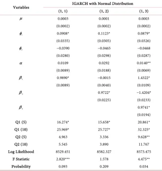
Finally we have given effort to model the volatility clustering in stock return addressing the restriction saying that “persistence parameters sum up to unit”. The rationale for this restriction is that earlier in some of the GARCH models it was found that the sum of the coefficients were close to or more than unit im-plying that the variance of stock return might be nonstationary. Imposing this

restriction in standard GARCH models leads to IGARCH specification. Table

A5 (Appendix) contains the estimation results of different IGARCH

specifica-tion with MA(2) condispecifica-tional mean model. As the results show IGARCH(1, 1) and also IGARCH(1, 3) have autocorrelation and ARCH effect. But the IGARCH(1, 2) have no autocorrelation in the squared residuals and also there is no ARCH effect. It also satisfies the imposed restriction and the significance of persistence parameter indicates that there is volatility clustering in stock market return. It also contains maximum likelihood (8582.32) and minimum informa-tion criteria (SIC = −5.8526) compared to the other two.

4.2. Out of Sample Forecasting Accuracy

(11)

[image:11.595.208.538.88.550.2]

Table 3. Estimation results for EGARCH model with MA specification.

Variables EGARCH with Normal Distribution (1, 1) (1, 2) (1, 3)

µ _0.0001 _0.0001 _0.0005**

(0.0002) (0.0003) (0.0002)

1

φ _0.1489* _0.1411* _0.1542*

(0.0220) (0.0226) (0.0222)

2

φ _0.0135 _0.0482*** _0.0325

(0.0556) (0.0260) (0.0580)

η _−1.2659* _−0.2956* _−0.5718*

(0.4370) (0.0737) (0.1038)

α 0.4865* 0.1611* 0.3038*

(0.1149) (0.0201) (0.0432)

λ −0.1527*** 0.0147 −0.0988**

(0.0914) (0.0090) (0.0526)

1

β _0.8945* _0.0200* _1.7725*

(0.0450) (0.0042) (0.0846)

2

β _0.9594* _−1.4774*

(0.0045) (0.1270)

3

β _0.6649*

(0.0408) Q1 (5) 21.938* 21.402* 27.451* Q1 (10) 28.350* 29.040* 33.939*

Q2 (5) 0.0892 25.218* 0.2585

Q2 (10) 0.2739 27.467* 1.0130

Log Likelihood 8744.181 8715.984 8815.427 F Statistic 0.0467 13.547* 0.0102 Probability 0.8288 0.000 0.9193 Note: Robust Standard Errors are in Parenthesis. *** indicates significant at 10 per cent level, ** indicates significant at 5 per cent level and * indicates that at 1 per cent level.

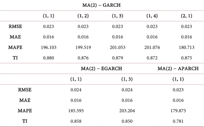
pseudo sample has been created using the observations for the period 27th

No-vember, 2001 to 30th_{December 2010. The forecasting accuracy of different}

mod-els was compared in terms of RMSE, MAE, MAPE and TI for the period 2nd

January 2011 to 31st_{July, 2013.}_{Table 4}_{contains the results. As it can be}

(12)

[image:12.595.208.539.90.296.2]

Table 4. Out of sample forecasting accuracy of different models.

MA(2) − GARCH

(1, 1) (1, 2) (1, 3) (1, 4) (2, 1) RMSE 0.023 0.023 0.023 0.023 0.023 MAE 0.016 0.016 0.016 0.016 0.016 MAPE 196.103 199.519 201.053 201.076 180.713

TI 0.880 0.876 0.879 0.872 0.875 MA(2) − EGARCH MA(2) − APARCH (1, 1) (1, 3) (1, 1)

RMSE 0.024 0.024 0.023

MAE 0.016 0.016 0.016

MAPE 185.595 203.204 179.875

TI 0.858 0.850 0.781

satisfies all the required restrictions and revealed the volatility clustering feature of stock return appropriately. Thus if the purpose is only modeling the volatility clustering and forecasting the future volatility then MA(2) − GARCH(2, 1) will perform better.

When we have tried to forecast the volatility in stock return while addressing the asymmetric affect it was found again that in terms of RMSE and MAE, MA(2) − EGARCH(1, 1), MA(2) − EGARCH(1, 3) and MA(2) − APARCH(1, 1) all are same. In terms of TI, MA(2) − EGARCH(1, 3) is better than MA(2) − EGARCH(1, 1) while its other way around in terms of MAPE. However, among EGARCH and APARCH, MA(2) − APARCH(1, 1) has the lowest value both for TI and MAPE. Nevertheless, earlier it was observed that APARCH model failed to capture the asymmetric volatility effect. Thus, if the purpose is to capture the asymmetric volatility effect along with forecasting then the appropriate model would be MA(2) − EGARCH(1, 3) as it was able to capture the asymmetric vola-tility effect appropriately. It also had maximum likelihood and minimum infor-mation criteria when full sample was used and have a lower TI value when out of

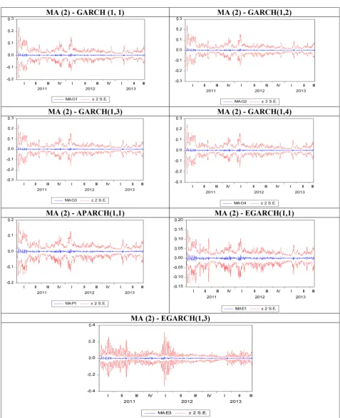
sample forecasting is considered. Figure A4 (Appendix) contains the forecasted

volatility along with the confidence interval for the aforementioned models.

5. Conclusions and Policy Relevance

(13)

Modeling of conditional variance of stock return also has greater relevance for taking decision by the investors and policy makers regarding portfolio optimiza-tion, asset pricing and finally risk management. An appropriate variance model will help concerned people to have a better forecast of volatility which in turn would be significant for having efficient portfolio distribution, better risk man-agement capacity and more specific derivative prices for particular financial in-strument.

Identifying appropriate volatility model for capturing fluctuations in stock returns is of significant policy relevance to the policy makers as well. The im-portance lies on the fact that unregulated fluctuation in asset return could influ-ence investment decision that can manifest in the real sector with adverse con-sequences for economic growth and development. Undue fluctuation of stock return could also impose challenges to monetary policy formulation as increase in stock prices stimulates interest rate which eventually could generate

inflatio-nary spree in the economy [23] [24]. In this regard, stabilization policy is

re-quired and the specification of optimal volatility model for capturing variations in stock returns makes a pre-condition for the monetary authority intervention.

In the above context this paper goes with challenge of exploring comparative ability of capturing in-sample and out-of-sample volatility of different condi-tionally heteroscedastic econometric models regarding stock market return in

Bangladesh. More specifically, it explored daily data for the period 27th

Novem-ber, 2001 to 31st_{July, 2013 from DSE and has used different GARCH class}

mod-els to compare their performance form in-sample estimation accuracy and out-of-sample forecasting accuracy perspective to come up with the best per-forming one. By developing appropriate mean equation for addressing the au-tocorrelation problem the paper compared different order of variance models namely, GARCH, APARCH, EGARCH and IGRACH. While concerning in sample estimation accuracy it was found that MA(2) − GARCH(2, 1) out per-forms AR(2) − GARCH(2, 1) following post estimation diagnostics. When non-linearity was allowed in variance equation to capture the asymmetric effect MA(2) − EGARCH(1, 3) was found to be successful over MA(2) − APARCH(1, 1). By assuming that variance could potentially be remained nonstationary it was observed that MA(2) − IGARCH(1, 2) has more in sample accuracy than its other counterparts. As far as out of sample volatility forecasting is concerned it was found that for only modeling the volatility clustering MA(2) − GARCH(2, 1) out performs the other. However, for modeling the volatility clustering address-ing the asymmetric effect MA(2) − EGARCH(1, 3) provides more out of sample accurate result among its competing ones. Therefore, it can be argued with evi-dence that there is no clear winner. The decision mainly depends on the purpose of the concerned people. From volatility persistency perspective MA(2) − GARCH(2, 1) is better due to both in sample and out of sample accuracy. In contrast, from capturing asymmetric effect perspective MA(2) − EGARCH(1, 3) is better.

(14)

in-DOI: 10.4236/tel.2018.814199 3216 Theoretical Economics Letters

corporate the issue of existence of structural break in the variance dynamics while modeling the conditional heteroscedasticity. Nevertheless, addressing the structural break in variance dynamics could remain as a further area of research.

Conflicts of Interest

The authors declare no conflicts of interest regarding the publication of this pa-per.

References

[1] Rajni, M. and Mahendra, R. (2007) Measuring Stock Market Volatility in an Emerging Economy. International Research Journal of Finance & Economics, 8, 126-133.

[2] Zuliu, H. (1995) Stock Market Volatility and Corporate Investment.IMF Working Paper, 95-102.

[3] Levine, R. and Zervous, S. (1996) Stock Market Development and Long-Run Growth. World Bank Economic Review,10, 323-339.

https://doi.org/10.1093/wber/10.2.323

[4] Olowe, R.A. (2009) Stock Return, Volatility & the Global Financial Crisis in an Emerging Market: The Nigerian Case. International Review of Business Research Papers,5, 426-447.

[5] Olowe, R.A. (2009) The Impact of the Announcement of the 2005 Capital Require-ment for Insurance Companies on the Nigerian Stock Market. The Nigerian Journal of Risk and Insurance,6, 43-69.

[6] Chowdhury, A.R. (1994) Statistical Properties of Daily Returns from the Dhaka Stock Exchange. The Bangladesh Development Studies, 22, 61-76.

[7] Basher, S.A., Hassan, M.K. and Islam, A.M. (2007) Time-Varying Volatility and Eq-uity Returns in Bangladesh Stock Market. Applied Financial Economics, 17, 1393-1407.https://doi.org/10.1080/09603100600771034

[8] Rayhan, M.A., Sarker, S.A. and Sayem, S.M. (2011) The Volatility of Dhaka Stock Exchange (DSE) Returns: Evidence and Implications. ASA University Review, 5, 97-99.

[9] Rahman, M.M., Huq, M.M. and Rahman, M.S. (2012) In Sample and Out of Sample Forecasting Performance under Fat Tail and Skewed Distribution. Proceeding Book of International Conference on Statistical Data Mining for Bioinformatics, Health,

Agricultural and Environment, Department of Statistics, University of Rajshahi, December 2012, 462-472.

[10] Islam, M., Ali, L.E. and Afroz, N. (2012) Forecasting Volatility of Dhaka Stock Ex-change: Linear Vs Non-Linear Models. International Journal of Science and Engi-neering, 3, 4-8.

[11] Huq, M.M., Rahman, M.M., Rahman, M.S., Shahin, M.M. and Ali, M. (2013) Anal-ysis of Volatility and Forecasting General Index of Dhaka Stock Exchange. Ameri-can Journal of Economics, 3, 229-242.

[12] Alam, M.Z., Siddikee, M.N. and Masukujjaman, M. (2013) Forecasting Volatility of Stock Indices with ARCH Model. International Journal of Financial Research, 4, 126-143.https://doi.org/10.5430/ijfr.v4n2p126

(15)

https://doi.org/10.18034/abr.v4i1.72

[14] Miah, M. and Rahman, A. (2016) Modelling Volatility of Daily Stock Returns: Is GARCH(1,1) Enough? American Scientific Research Journal for Engineering,

Technology, and Sciences (ASRJETS), 18, 29-39.

[15] Uddin, M., Islam, M.S. and Majumder, M.A. (2016) Market Efficiency, Time-Varying Volatility and Equity Returns in the Dhaka Stock Exchange. World Review of Busi-ness Research, 6, 43-62.

[16] Bollerslev, T. (1986) Generalised Autoregressive Conditional Heteroskedasticity.

Journal of Econometrics, 31, 307-327.

https://doi.org/10.1016/0304-4076(86)90063-1

[17] Erdemlioglu, D., Laurent, S. and Neely, C.J. (2012) Econometric Modeling of Ex-change Rate Volatility and Jumps. Working Paper, Federal Reserve Bank of St. Louis.

[18] Engle, R.F. (1982) Autoregressive Conditional Heteroskedasticity with Estimates of the Variance of United Kingdom Inflation. Econometrica, 50, 987-1007.

https://doi.org/10.2307/1912773

[19] Ding, Z., Granger, C.W. and Engle, R.F. (1993) A Long Memory Property of Stock Market Returns and a New Mode. Journal of Empirical Finance, 1, 83-106.

https://doi.org/10.1016/0927-5398(93)90006-D

[20] Nelson, D. (1991) Conditional Heteroskedasticity in Asset Returns: A New Ap-proach. Econometrica, 59, 347-370.https://doi.org/10.2307/2938260

[21] Dickey, D.A. and Fulle, W.A. (1979) Distribution of the Estimators for Autoregres-sive Time Series with a Unit Root. Journal of the American Statistical Association, 74, 427-431.https://doi.org/10.1080/01621459.1979.10482531

[22] Kwiatkowski, D., Phillips, P.C., Schmidt, P. and Shin, Y. (1992) Testing the Null Hypothesis of Stationarity against the Alternative of a Unit Root: How Sure Are We That Economic Time Series Have a Unit Root? Journal of Econometrics, 54, 159-178.https://doi.org/10.1016/0304-4076(92)90104-Y

[23] Fischer, S. (1981) Relative Stocks, Relative Price Variability, and Inflation. Brook-ings Paper on Economic Activity, 1981, 381-441.https://doi.org/10.2307/2534344

[24] Veronesi, P. (1999) Market Overreactions to Bad News in Good Times: A Rational Expectations Equilibrium Model. The Review of Financial Studies, 12, 975-1007.

(16)

[image:16.595.60.542.294.703.2]

Appendix

Table A1. Summary statistics of DSE index.

Variable Mean Median Std. Deviation Skewness Kurtosis DSE General Index 2810.734 2074.550 1935.526 0.897 2.847

Table A2. Staionarity test results for the stock return series.

Augmented Dickey Fuller (ADF) Test Kwiatkowski –Philips–Schmidt–Shin (KPSS) Test H0: Stock Return has a Unit Root H0: Stock Return is Stationary

Intercept Trend and Intercept Intercept Trend and Intercept Test Statistic Probability Test Statistic Probability Test Statistic 1% Critical Value Test Statistic 1% Critical Value

−52.0260* 0.0000 −52.0246 0.0000 0.174 0.739 0.133 0.216 Optimum Order of Lag is Zero Optimum Order of Lag is Zero Optimum Bandwidth is Nine Optimum Bandwidth is Eight Note: *indicates significant at 1% level. In case of selecting optimal lag length for ADF test, the SIC has been minimized. The optimum bandwidth for KPSS test has been selected using Newey-West method and following Bartlett Kernel for spectral estimation.

Table A3. Estimation results of GARCH models with AR mean specification.

Coefficients GARCH

(1, 1) (1, 2) (1, 3) (1, 4) (1, 5) (2, 1)

µ _0.0014** _0.0014** _0.0031* _0.0013** _0.0012*** _0.0012**

(0.0006) (0.0006) (0.0003) (0.0006) (0.0006) (0.0005)

1

θ 0.0812*** 0.0936*** 0.0313 0.0950*** 0.1005** 0.1039** (0.0483) (0.0507) (0.0388) (0.0531) (0.0512) (0.0477)

2

θ −0.0310 −0.0391 −0.0319 −0.0290 −0.0352 −0.0360 (0.0402) (0.0460) (0.0236) (0.0548) (0.0543) (0.0492)

η _1.25E−05 _9.83E−06* _3.53E−05* _5.29E−06* _3.50E−06* _1.27E−05**

(7.68E−06) (3.08E−06) (2.84E−06) (1.79E−06) (6.07E−07) (5.87E−06)

1

α 0.3458* 0.3187* 0.3498* 0.2738* 0.2282** 0.1829** (0.1111) (0.0703) (0.0341) (0.0878) (0.0911) (0.0841)

2

α 0.4092

(0.3770)

1

β 0.6695* 0.9743* 0.9816* 1.4296* 1.7836* 0.5187* (0.0791) (0.0821) (0.1204) (0.1068) (0.0961) (0.1580)

2

β _−0.2596* _−0.4264* _−1.1306* _−1.9036*

(0.0812) (0.0910) (0.1831) (0.1880)

3

β 0.0732* 0.5869* 1.5081*

(0.0160) (0.1394) (0.2141)

4

β _−0.1099** _−0.8152*

(0.0548) (0.1469)

5

β 0.2462*

(0.0517)

Q1 (5) 35.381* 34.211* 48.953* 37.973* 35.341* 34.203* Q1 (10) 41.864* 41.195* 56.104* 45.295* 45.573* 42.249* Q2 (5) 0.1167 0.1709 0.1029 0.1291 0.141 0.227 Q2 (10) 0.3078 0.3840 0.3891 0.449 0.423 0.601 Log Likelihood 8693.102 8710.725 8584.991 8733.666 8743.978 8739.313

F Stat. 0.0518 0.0564 0.024 0.058 0.040 0.013

Prob. 0.8199 0.8122 0.874 0.809 0.841 0.906

(17)

[image:17.595.216.538.90.467.2]

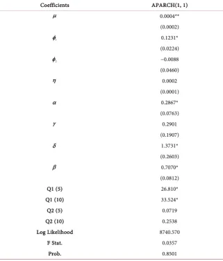
Table A4. APARCH with MA mean specification.

Coefficients APARCH(1, 1)

µ _0.0004**

(0.0002)

1

φ 0.1231*

(0.0224)

2

φ −0.0088

(0.0460)

η _0.0002

(0.0001)

α 0.2867*

(0.0763)

γ _0.2901

(0.1907)

δ 1.3731*

(0.2603)

β 0.7070*

(0.0812)

Q1 (5) 26.810*

Q1 (10) 33.524*

Q2 (5) 0.0719

Q2 (10) 0.2538

Log Likelihood 8740.570

F Stat. 0.0357

Prob. 0.8501

(18)

[image:18.595.209.538.90.437.2]

Table A5. Estimation results for IGARCH model with MA mean specification.

Variables IGARCH with Normal Distribution (1, 1) (1, 2) (1, 3)

µ _0.0003 _0.0001 _0.0003

(0.0002) (0.0002) (0.0002)

1

φ 0.0908* 0.1123* 0.0879*

(0.0335) (0.0305) (0.0326)

2

φ −0.0390 −0.0465 −0.0468

(0.0280) (0.0298) (0.0287)

α 0.0109 0.0292 0.0140**

(0.0089) (0.0188) (0.0069)

1

β 0.9890* −0.0015 1.4322*

(0.0089) (0.0040) (0.0109)

2

β 0.9722* −1.4204*

(0.0225) (0.0233)

3

β 0.9741*

(0.0194) Q1 (5) 16.274* 15.658* 20.861* Q1 (10) 25.969* 25.727* 32.325*

Q2 (5) 4.963 3.336 9.628**

Q2 (10) 5.545 3.890 11.767

Log Likelihood 8529.451 8582.327 8573.475 F Statistic 2.820*** 1.578 4.475**

Probability 0.093 0.209 0.034

(19)

[image:19.595.58.537.71.252.2]

[image:19.595.229.370.291.387.2]

Figure A1. Time series graph of DSE general index and DSE stock return.

Figure A2. Correlogram of the stock return.

Figure A3. Volatility clustering of stock market return.

[image:19.595.59.538.422.601.2]

(20)

[image:20.595.60.538.61.648.2]