ISSN Online: 2163-0496 ISSN Print: 2163-0461
DOI: 10.4236/ojmh.2018.83007 Jul. 17, 2018 83 Open Journal of Modern Hydrology
Detection of Spatial, Temporal and Trend of
Meteorological Drought Using Standardized
Precipitation Index (SPI) and Effective Drought
Index (EDI) in the Upper Tana River Basin,
Kenya
Raphael M. Wambua
1*, Benedict M. Mutua
2, James M. Raude
31Department of Agricultural Engineering, Egerton University, Nakuru, Kenya 2Division of Planning, Research and Innovation, Kibabii University, Bungoma, Kenya 3Jomo Kenyatta University of Agriculture & Technology, Juja, Kenya
Abstract
Drought events across the world are increasingly becoming a critical problem owing to its negative effects on water resources. There is need to understand on-site drought characteristics for the purpose of planning mitigation meas-ures. In this paper, meteorological drought episodes on spatial, temporal and trend domains were detected using Standardized Precipitation Index (SPI) and Effective Drought Index (EDI) in the upper Tana River basin. 41 years (1980-2016) monthly precipitation data from eight meteorological stations were used in the study. The SPI and EDI were used for reconstruction of the drought events and used to characterize the spatial, temporal and trend dis-tribution of drought occurrence. Drought frequency was estimated as the ratio of a defined severity to its total number of events. The change in drought events was detected using a non-parametric man-Kendall trend test. The main drought conditions detected by SPI and EDI are severe drought, moderate drought, near normal, moderate wet, very wet and extremely wet conditions. From the results the average drought frequency between 1970 and 2010 for the south-eastern and north-western areas ranged from 12.16 to 14.93 and 3.82 to 6.63 percent respectively. The Mann-Kendall trend test show that drought trend increased in the south-eastern parts of the basin at 90% and 95% significant levels. However, there was no significant trend that was de-tected in the North-western areas. This is an indication that the south-eastern parts are more drought-prone areas compared to the North-western areas of the upper Tana River basin. Both the SPI and the EDI were effective in de-How to cite this paper: Wambua, R.M.,
Mutua, B.M. and Raude, J.M. (2018) Detec-tion of Spatial, Temporal and Trend of Meteorological Drought Using Standard-ized Precipitation Index (SPI) and Effective Drought Index (EDI) in the Upper Tana River Basin, Kenya. Open Journal of Mod-ern Hydrology, 8, 83-100.
https://doi.org/10.4236/ojmh.2018.83007
Received: May 7, 2018 Accepted: July 14, 2018 Published: July 17, 2018
Copyright © 2018 by authors and Scientific Research Publishing Inc. This work is licensed under the Creative Commons Attribution International License (CC BY 4.0).
http://creativecommons.org/licenses/by/4.0/
DOI: 10.4236/ojmh.2018.83007 84 Open Journal of Modern Hydrology tecting the on-set of drought, description of the temporal variability, severity and spatial extent across the basin. It is recommended that the findings be adopted for decision making for drought-early warning systems in the river basin.
Keywords
SPI, EDI, Drought-Detection, Man-Kendall, Drought-Prone Areas, Drought Frequency, Drought-Early Warning System, Upper Tana River Basin
1. Introduction
Drought is a natural phenomenon associated with deficit of water availability resulting from low precipitation compared to long term average [1] and can be described on s spatial domain [2]. Drought has become more frequent and se-vere in arid and semi-arid lands (ASALS) than in humid areas. Drought is a dis-aster which affects large areas and for a longer period compared to other natural disasters such as floods. Globally, drought has become more common with a number of countries experiencing drought of different characteristics. Different regions experience droughts which have different spatial and temporal characte-ristics. It is critical to detect spatial, temporal as well as trend characteristics of different droughts such as the meteorological droughts for a well-coordinated mitigation planning. The meteorological drought which is the most commonly known drought is associated with long time intervals of significantly low or no precipitation and increased air temperature. The deficiency in rainfall leads into low infiltration, decreased runoff and ground water recharge. On the other hand, high air temperatures lead to changes in wind characteristics such as increased wind velocity, low Relative Humidity (RH) and increased evapo-transpiration (ET).
1.1. Indices for Met-Drought
A number of drought indices have been developed and applied in met-drought assessment over the years. Some of these indices include Aggregated Drought Index (ADI) [3], Standardized Precipitation Index (SPI) [4][5], Palmer Drought Severity Index (PDSI) and Z-Index [6], Effective Drought Index (EDI) [7], Keetch-Byram Drought Index (KBDI) [8], Hybrid Drought Index (HDI) [9], Vegetation Drought Response Index (VegDRI) [10], Recconnaissance Drought Index (RDI) [11], Rainfall Anormally Index (RAI) [12], Drought Severity Index (DSI) [13], National Rainfall Index (NRI) [14] and Drought frequency index (DFI) [15]. Among the mereorological drought indices, the SPI and EDI have generally been used more than most of the other drought indices because they require precipitation as a single input variable.
1.2. Standardized Precipitation Index
DOI: 10.4236/ojmh.2018.83007 85 Open Journal of Modern Hydrology precipitation deficit and monitor drought conditions within Colorado, USA. The SPI is used to categorize the different drought classes as described in [4]. For calculation of SPI, long-term historical precipitation record of at least 30 years is integrated into a probability distribution function which is then transformed in-to a normal distribution function. The SPI requires less input data compared in-to most other drought indices and this makes it flexible for wide applications [16] [17]. The SPI has several advantages which make it more applicable in many river basins. First, it requires only the precipitation as the input data. This makes it ideal for river basins that do not have extensive hydrological data records. Se-condly, its evaluation is relatively easy since it uses precipitation data set only. Thirdly, it is a standardized index and this makes it independent of geographical location as it is based on average precipitation values derived from the area of interest. In addition, the SPI exhibits statistical consistency, and has the ability to present both short-term and long-term droughts over time scales of precipita-tion variaprecipita-tion [18]. However, the SPI has some disadvantages in its use as a drought assessment tool. First, it is not always easy to find a probability distribu-tion funcdistribu-tion to fit and model the raw precipitadistribu-tion data. Secondly, most river basins do not have reliable time-series data to generate the best estimate of the distribution parameters. In addition, application of SPI in arid and semi-arid lands of time-series of less than three months may give inaccurate values.
To overcome the challenge of simulating and modelling the data for SPI out-puts, application of different probability distribution functions may be employed. These include the Gamma, Pearson type III, Lognormal, Extreme Value and Exponential distribution functions [19]. However, the Gamma probability dis-tribution function is preferred in hydrological studies. In hydrology, it has an advantage of fitting only positive and zero values since hydrological variables such as precipitation, and runoff are always positive or equal to zero as lower limit values [20][21]. The Gumbel and Weibull distribution functions are used for study of extreme hydrological variables. The Gumbel distribution function is used for frequency analysis of floods, while the Weibull distribution function is used to analyze low flow values observed in rivers. SPI has been found to per-form differently for various time scales. For time scales shorter than 6 months, there is insignificant autocorrelation while for time scales greater than 6 months, the autocorrelation increases significantly [22].
1.3. Effective Drought Index
The effective drought index (EDI) uses effective precipitation which is the ac-cumulation of selected portions of the days before the estimated time period [19]. It estimates droughts more accurately than many other indices in terms of on-set, detection, spatial and temporal analysis. When compared with seven other drought indices in Iran, [23] found that EDI is more accurate and consistent in the study of drought.
DOI: 10.4236/ojmh.2018.83007 86 Open Journal of Modern Hydrology occur. There is need to understand drought spatial, temporal and trend charac-teristics for its prioritized integration in planning for timely mitigation measures. In this paper therefore, meteorological drought on spatial, temporal and trend domains was detected using Standardized Precipitation Index (SPI) and Effective Drought Index (EDI) for the upper Tana River basin with a view for its incorpo-ration in drought early warning systems.
2. Materials and Methods
2.1. Study Area
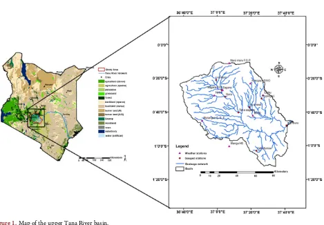
The upper Tana River basin has an area of 17,420 km2 as presented in Figure 1 and is the focus of this study. The basin lies between latitudes 00˚05' and 01˚30' south and longitudes 36˚20' and 37˚60' east. The upper Tana River basin lies between latitudes 00˚05' and 01˚30' south and longitudes 36˚20' and 37˚60' east.
The basin has forest land resources located along the eastern slopes of Mount Kenya and Aberdares range which are crucial in controlling hydrological processes of the basin [24]. This basin is located in a fragile ecosystem with all agro-ecological zones of Kenya. The Tana River tributaries originate from the slopes of Mount Kenya and Aberdares range. The basin constitutes a very im-portant resource in Kenya such as being a water supply source, hydro-power generation and agricultural production.
2.2. Standardized Precipitation Index
The Standardized Precipitation Index (SPI) was used to quantify precipitation deficit within the basin as a representation of drought condition as defined by [4]. The first step involved fitting the precipitation data into a probability distri-bution function and then computation of the SPI values. The computed SPI val-ues were used in drought assessment and classification. In the first step, the gamma distribution function was adapted since it fits well in time series precipi-tation data [25]. The gamma distribution is expressed in terms of its probability density function as:
(
, ,)
1( )
1e x for , , 0f x xα β x
α
α β α β
β α
− −
= >
Γ (1)
where; α = the shape parameter, β = scale parameter, x = the precipitation amount (mm), Γ(α) = the value taken by gamma function and
x
= mean rain-fall (mm).The Γ(α) is the value defined by the Gamma function which is determined by applying an integral function according to [11] expressed as:
( )
10
e dy
x x
α α
α − −
Γ =
∫
(2)where; Γ(α) = the value taken by gamma function, x = the precipitation amount (mm) and α = the shape parameter.
DOI: 10.4236/ojmh.2018.83007 87 Open Journal of Modern Hydrology
Figure 1. Map of the upper Tana River basin.
maximum probability was then used to estimate the optimal values of α and β
using Equations (3) and (4):
1 1 1 4
4 3
A A
α = + +
(3)
x
β
α
= (4)
where; α = the shape parameter, β = scale parameters,
x
= mean precipitation (mm) and A = sample statistic.The sample statistic is defined as:
( )
lnln x
A x
n
= − (5)
where;
x
= the precipitation average (mm) and n = the number of observa-tionsThe calculated values were in turn used to compute the cumulative probability for non-zero rainfall using Equations (6) and (7) respectively:
(
)
(
)
( )
10 0
1
, , x , , d x e x d
f x f x x xα β x
α
α β α β
β α − −
= =
Γ
∫
∫
(6)where; α= the shape parameter, β = scale parameter and x = the precipitation amount (mm)
DOI: 10.4236/ojmh.2018.83007 88 Open Journal of Modern Hydrology
(
)
( )
10
1
, , x e d fort x
f xα β tα t t
α − β
= =
Γ
∫
(7)where; Γ(α) = the value taken by gamma function, x = the precipitation amount (mm), β = scale parameter and t = the time period
The Gamma function was applied for values of precipitation x > 0 for the pre-cipitation time series of the upper Tana River basin. In case of non-zero values, cumulative probability of both zero and non-zero values were computed. This probability is represented by a function H(x) defined as:
( )
(
1) (
, ,)
H x = + −q q F x
α β
(8)where; H(x) = Cumulative probability and q = probability of zero precipitation When m was taken as the number of zero entries in the time series precipita-tion data, then the q value was estimated by the ratio m/n. The cumulative probability was then transformed into a standard normal distribution function. This gave values of the mean and variance of the SPI as zero and one respectively. This step was carried out using approximate transformation functions adapted from [26]. These functions given in Equations (9) and (10) are expressed as:
( )
20 1 2
2 3
1 2 3
for 0 0.5
1
c c k c k
SPI k H x
d k d k d k
+ +
= − − < ≤
+ + +
(9)
( )
20 1 2
2 3
1 2 3
for 0.5 1.0
1
c c k c k
SPI k H x
d k d k d k
+ +
= + − < <
+ + +
(10)
where; c0 = 2.515517, c1 = 0.802853, c2 = 0.010328, d1 =1.432788, d2 = 0.189269,
d3 = 0.001308
The parameters were used to compute the SPI and were adapted from [19]. The value of k in Equations (9) and (10) was determined from the functions given as:
( )
2( )
1
ln for 0 0.5
k H x
H x
= < ≤
(11)
( )
2( )
1
ln for 0.5 1.0
1
k H x
H x
= < <
−
(12)
In this study, the SPI values were calculated using a monthly time step and the threshold ranges adapted from [25] ranging from extreme drought to extremely wet conditions.
2.3. Effective Drought Index
DOI: 10.4236/ojmh.2018.83007 89 Open Journal of Modern Hydrology 1
1
m m N
i P
m
PE ED
m
= =
=
∑
∑
(13)where; EPp =effective precipitation parameter (mm), m = total period before the current month, PEm = the precipitation in m − 1 months before the current month (mm) and N = duration of summation of the precipitation.
The mean EP is computed annually to represent the climatological characte-ristics of water resources. For practical application of MEP a 5-months running mean is applied in this computation [28]. Then the deviation time series EP
from the mean EP was computed using the relation:
DEP EP MEP= − (14) where; DEP = deviation of time series EPpfrom mean effective precipitation pa-rameter (mm) and MEP = mean effective precipitation parameter (mm)
From the EPp, both the mean and the standard deviations of the monthly val-ues were determined. The resulting time-series EP was used as inputs to calcu-late its deviation from the mean. Then the return to normal precipitation (RNP) values was determined using the relation adopted from [29]:
1 DEP RNP
N =
∑
(15)where; RNP = return to normal precipitation (mm)
N = previous period (months)
From the calculated RNP, the EDI was derived from the relation:
(
)
RNP EDI
Std RNP
= (16)
where; Std (RNP) = Standard deviation of a particular months RNP values Using the computed EDI values, the severity of the drought was categorized based on the thresholds and classification (ranging from extreme drought to ex-treme wet conditions) adopted from [30].
2.4. Mann-Kendall Trend Test for Drought Conditions
DOI: 10.4236/ojmh.2018.83007 90 Open Journal of Modern Hydrology
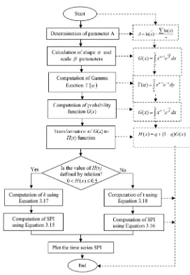
Figure 2. Process for computation of the time series SPI.
(
)
1
1 1
n n
i k
k j k
S = sign x x
= = +
= −
∑ ∑
(17)The right hand side of the Equation (17) was simplified using Equation (18) given as:
(
)
(
(
)
)
(
)
1 if 0
0 if 0
1 if 0
j k
j k j k
j k
x x
sign x x x x
x x
− >
− = − =
− − <
(18)
The probability linked to the Mann-Kendall statistic S and the selected n-data were determined to quantify the level of significance of the trend. The VAR(S) was calculated and then the normalized test statistic Z was computed using the following equations:
( )
1 2(
5)
(
1 2 5)(
)
18
t
t t t
VAR S =n n − n+ − − +
DOI: 10.4236/ojmh.2018.83007 91 Open Journal of Modern Hydrology
( )
( )
1 if 0
0 if 0
1 if 0
S S
VAR S
Z S
S S
VAR S −
>
= =
+
<
(20)
where; VAR(S) = the variance of the data set and n = the number of data points Equation (20) which was adapted from [35] was used to qualify the drought trend in the basin as: no trend, increasing trend and decreasing trend when S = 0,
S > 0 and S < 0 respectively. In order to determine whether or not the drought trend in the upper Tana River basin was significant or insignificant, significance levels at 90% and 95% were used. At these significance levels, the null hypothesis of no trend was rejected when Z >1.645 and Z >1.96 respectively where the values of Z were adapted from [36].
3. Results and Discussions
3.1. Time Series SPI
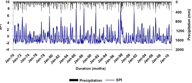
The results for monthly time series SPI and the spatial characteristics of drough-ts in the upper Tana River basin are presented. The resuldrough-ts spatial maps are based on the partitioned basin into four elevations bands; low, lower-middle, middle and high elevations. The results of plotted drought conditions on monthly time series graphs are illustrated using the graphs for meteorological stations Sagana FCF (ID 9037096), Kerugoya DWO (ID 9037031), Nyeri (ID 9036288) and Naro-moru (ID 9037064) as presented in Figures 3-6.
DOI: 10.4236/ojmh.2018.83007 92 Open Journal of Modern Hydrology
[image:10.595.213.538.250.364.2]Figure 3. Time series SPI and precipitation for Sagana FCF meteorological station.
Figure 4. Time series SPI and precipitation at Kerugoya DWO meteorological station.
Figure 5. Time series SPI and precipitation for Nyeri meteorological station.
Figure 6. Time series SPI and precipitation for Naro-moru meteorological station.
0 200 400 600 800 1000 1200 1400 1600 -4
-2 0 2 4 6 8 10
Pr
ec
ip
ita
tio
n (
mm)
SP
I
Duration (months)
[image:10.595.213.537.401.526.2] [image:10.595.213.538.564.705.2]DOI: 10.4236/ojmh.2018.83007 93 Open Journal of Modern Hydrology
3.2. Spatially Distributed Drought Severity Based on SPI
Drought severities for the upper Tana River basin were computed and mapped using the Kriging approach for the selected years; 1970, 1980, 1990, 2000 and 2010. From Figure 7, it is observed that the spatial drought distribution in the south-eastern areas of the basin exhibit drought severities ranging from 2.044 to 2.835 and from 4.416 to 5.207. In addition, the results show that the north- western parts of the basin experienced drought severity values of 1.822 to 2.463 and 3.745 to 4.384 for 1970 and 2010 respectively. These results indicate that the south-eastern parts of the basin exhibit the highest drought severities while the north-western areas have the lowest. The spatial variation of drought is compa-rable with the drought distribution generated in other river basins for instance by [37] in the Tel river basin and [6] in the upper Seonath sub-basin.
Based on the SPI, the areal-extend of drought severities increased in both the South-eastern and North-western areas from 4868.7 km2 to 6880 km2, and 6163.9 km2 to 6985.5 km2 from 1970 to 2010 respectively. Between 1970 and 1980, the drought areal-extend is almost the same but a significant increase oc-curred between 1980 and 2010.
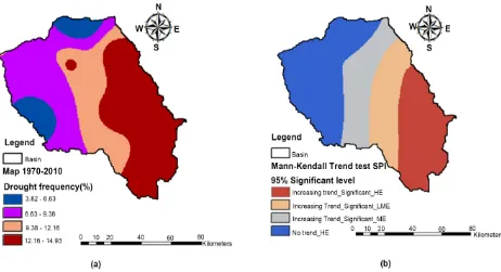
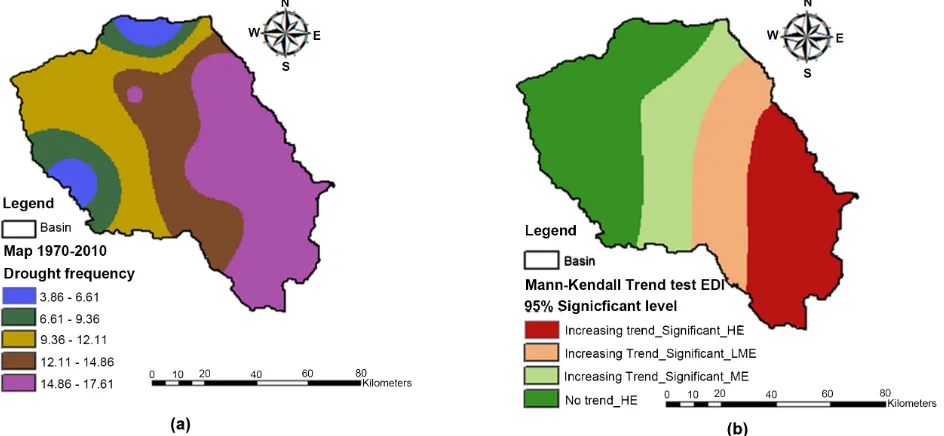
From Figure 8(a), the results show that the average drought frequency be-tween 1970 and 2010 for the South-eastern and North-western areas ranged from 12.16 to 14.93 and 3.82 to 6.63 respectively. The drought characteristics were also subjected to Mann-Kendall trend test across the basin. Results of the Mann-Kendall test show that drought trend increased in the South-eastern parts of the basin at 90% and 95% significant levels. However, the results given in Figure 8(b) shows that there was no significant trend that was detected in the North-western areas. This is an indication that the South-eastern parts are drought-prone areas compared to the North-western areas of the upper Tana River basin.
3.3. Monthly Time Series EDI
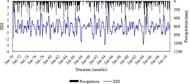
Monthly time series of EDI for meteorological stations Nyeri (ID 9036288), Ke-rugoya DWO (ID 9037031), Sagana FCF (ID 9037096) and Naro-moru (ID 9037064) are presented in Figures 9-12.
The results of the monthly time series EDI show that this index can be used to detect both the drought and wetness for different years. Typical droughts as presented by this index include the extreme droughts represented by the nega-tive values of −2.5, −2.2, −2.2, −2.5, −2.5, and −2.5 for the years 1972, 1973, 1992, 1994, 2000 and 2010 respectively. At the same time, the index was used to detect the wet conditions of the basin where positive values of +3.0, +3.0 and 4.3 for the years 1986, 1989 and 1998 respectively as illustrated by Figures 9-12 indicate wetness.
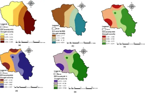
3.4. Spatially Distributed Drought Severity Based on EDI
DOI: 10.4236/ojmh.2018.83007 94 Open Journal of Modern Hydrology
Figure 7. (a)-(e): Spatially distributed drought severity based on SPI.
[image:12.595.65.527.455.706.2]DOI: 10.4236/ojmh.2018.83007 95 Open Journal of Modern Hydrology
[image:13.595.210.539.270.415.2]Figure 9. Time series EDI and precipitation for Nyeri meteorological station.
Figure 10. Time series EDI and precipitation for Kerugoya DWO meteorological station.
Figure 11. Time series EDI and precipitation for Sagana meteorological station.
those determined using the SPI. It is also noted that the drought severity values in South-eastern areas of the basin range from 3.850 to 4.486 and 4.804 to 5.584 in 1970 and 2010 respectively. Based on the spatially distributed EDI from 1970 to 2010, drought severity has shown some significant increase as per the Figure 13.
For the North-western parts, these values range from 1.822 to 2.463 and 3.745 to 4.384 for the years 1970 and 2010 respectively. Although the drought severity
[image:13.595.211.538.454.599.2]DOI: 10.4236/ojmh.2018.83007 96 Open Journal of Modern Hydrology
Figure 12. Time series EDI and precipitation for Naro-moru meteorological station.
Figure 13. (a)-(e): Spatially distributed drought severity based on EDI.
based on EDI is generally higher than the SPI, both indices exhibit similar trends in terms of spatial distribution, frequency and Mann-Kendall trend test as given in Figure 14(a) and Figure 14(b).
4. Conclusion
Different spatial and temporal drought conditions; severe drought, moderate drought, near normal, moderate wet, very wet and extremely wet conditions were detected using SPI and EDI for the Upper Tana River basin. The findings indicate that the South-eastern parts are more drought-prone areas compared to
[image:14.595.68.534.255.558.2]DOI: 10.4236/ojmh.2018.83007 97 Open Journal of Modern Hydrology
Figure 14. Spatially distributed (a) drought frequency based on SPI and (b) Mann-Kendall trend test of drought based on SPI.
the North-western areas of the upper Tana River basin. This is because in the South-eastern areas of the basin, spatial drought distribution exhibit drought severities ranging from 2.044 to 2.835 and from 4.416 to 5.207. In addition, the results show that the North-western parts of the basin experienced drought se-verity values of 1.822 to 2.463 and 3.745 to 4.384 for 1970 and 2010 respectively. From the results the average drought frequency between 1970 and 2010 for the South-eastern and North-western areas ranged from 12.16 to 14.93 and 3.82 to 6.63 respectively. The Mann-Kendall trend test showed that drought trend in-creased in the South-eastern parts of the basin at 90% and 95% significant levels. The trend showed that there was no significant trend that was detected in the North-western areas. This study can be applied in other river basins and the re-sults compared with the present findings.
Acknowledgements
The authors of this paper appreciate the African Development Bank (AfDB) for scholarship accorded to the corresponding author to undertake postgraduate studies. The authors also express their gratitude to the reviewers for useful comments on the manuscript. In addition, the editorial board that accepted the publication is greatly acknowledged. Egerton University, Division of Research and Extension is appreciated for resources support needed for publication of the article.
References
As-DOI: 10.4236/ojmh.2018.83007 98 Open Journal of Modern Hydrology
sessment and Mapping in Upper Seonath Sub-Basin Using GIS. International Jour-nal of Emerging Technology and Advanced Engineering, 4, 210-218.
[3] Keyantash, J.A. and Dracup, J.A. (2004) An Aggregate Drought Index: Assessing Drought Severity Based on Fluctuations in the Hydrologic Cycle and Surface Water Storage. Journal of Water Resources Research, 40, 1-14.
https://doi.org/10.1029/2003WR002610
[4] Mckee, T.B., Doesken, N.J. and Kleist, J. (1993) The Relationship of Drought Fre-quency and Duration to Time Scales. Proceedings of 8th Conference on Applied Climatology, Anaheim, 179-184.
[5] Vicente-Serano, S.M., Begneria, S. and Lopez-Moreno, J.I. (2010) A Multi-Scalar Drought Index Sensitive to Global Warming, the Standardized Precipitation Evapotranspiration Index. Journal of Climatology, 23, 1696-1711.
https://doi.org/10.1175/2009JCLI2909.1
[6] Palmer, W.C. (1965) Meteorological Drought Research Paper 45. Weather Bureau, Washington DC.
[7] Park, J.H., Kim, K.B. and Chang, Y. (2014). Statistical Properties of Effective Drought Index (EDI) for Seoul, Busan, Daegu, Makpo in South Korea. Asia-Pacific Journal of Atmospheric Science, 50, 453-458.
[8] Keetch, J.J. and Byuram, C.M. (1968) A Drought Index for Forest Fire Control, Res. Pap, SE-38. US Department of Agriculture, Forest Service, South Eastern Forest Experimental Station, Asheville.
[9] Karamouz, M., Rasouli, K. and Nazi, S. (2009) Development of a Hybrid Index for Drought Prediction: Case Study. Journal of Hydrologic Engineering, 14, 617-627. https://doi.org/10.1061/(ASCE)HE.1943-5584.0000022
[10] Brown, J.F., Wardlow, B.D., Tadesse, T., Hayes, M.J. and Reed, B.C. (2008) The Vegetation Drought Response Index (VegDRI). A New Integrated Approach for Monitoring Drought Stress in Vegetation. Geosciences and Remote Sensing, 45, 16-46.
[11] Tsakiris, G. and Vangelis, H. (2005) Establishing a Drought Index Incorporating Evapo-Transpiration. European Water Journal, 9, 3-11.
[12] Van-rooy, M.P. (1965) A Rainfall Anomaly Index (RAI), Independent of the Time and Space. Notos, 14, 43-48.
[13] Bryant, S., Arnell, N.W. and Law, F.M. (1992) The Long-Term Context for the Cur-rent Hydrological Drought. Proceedings of the IWEM Conference on the Manage-ment of Scarce Water Resources, Brighton, 13-14 October 1992.
[14] Gommes, R.A. and Petrassi, F. (1994) Rainfall Variability and Drought in Sub-Saharan Africa since 1960. FAO Agromet Report Series WP9, Rome.
[15] Gonzalez, J. and Valdes, J. (2006) New Drought Frequency Index, Definitions and Evaporative Performance Analysis. Water Resources Research,42, 333-349. https://doi.org/10.1029/2005WR004308
[16] Mckee, T.B. and Edwards, D.C. (1997) Characteristics of 20th Century Droughts in
the United States at Multiple Time Scales. Journal of Atmospheric Science, 634, 97-92.
[17] Bacanli, U.G., Firat, M. and Dikbas, F. (2008) Adaptive Neuro-Fuzzy Inference Sys-tem for Drought Forecasting. Journal of Stochastic Environmental Research and Risk Assessment,23, 1143-1154.
DOI: 10.4236/ojmh.2018.83007 99 Open Journal of Modern Hydrology
Regression. Journal of Applied Computational Intelligence and Soft Computing, 2012, Article ID: 794061.
[19] Byun, H.R. and Wilhite, D.A. (1999) Objective Quantification of Drought Severity and Duration. Journal of Climatology, 12, 2747-2756.
https://doi.org/10.1175/1520-0442(1999)012<2747:OQODSA>2.0.CO;2
[20] Markovic, R.D. (1965) Probability Functions of the Best Fit to Distributions of An-nual Precipitation and Runoff Hydrology. Paper No. 8, Colorado State University, Fort Collins.
[21] Aksoy, H. (2000) Use of Gamma Distribution in Hydrological Analysis. Turkish Journal of Engineering Sciences, 24, 419-428.
[22] Awass, A.A. (2009) Hydrological Drought Analysis-Occurrence, Severity and Risks, the Case of Wabi Shebele River Basin. Ethiopia PhD Thesis, Universität Siegen, Siegen.
[23] Morid, S., Smakhtin, V. and Moghaddasi, M. (2006) Comparison of Seven Mete-orological Indices for Drought in Iran. International Journal of Climatology, 26, 971-985.https://doi.org/10.1002/joc.1264
[24] IFAD (2012) Upper Tana Catchment Natural Resource Management Project. Re-port, East and Southern Africa Division, Project Management Department. [25] Cassiamani, C., Morgillo, A., Marchesi, S. and Pavan, V. (2007) Monitoring and
Forecasting Drought on a Regional Scale: Emilia Romagna Region. Water Science and Technology, 62, 29-48.
[26] Mishra, A.K., Desai, V.R. and Singh, V.P. (2007) Drought Forecasting Using a Hy-brid Stochastic and Neural Net-Work Models. Journal of Hydrological Engineering, 12, 626-638.https://doi.org/10.1061/(ASCE)1084-0699(2007)12:6(626)
[27] Smakhtin, V.U. and Hughes, D.A. (2007) Automated Estimation and Analysis of Meteorological Drought Characteristics from Monthly Rainfall Data. Journal Envi-ronmental Modelling and Software, 22, 880-890.
[28] Bulu, A. and Aksoy, H. (1998) Low Flow and Drought Studies in Turkey. Proceed-ings of Low Flows Expert Meeting, Belgrade, 10-12 June 1998.
[29] Roudier, P. and Mahe, G. (2010) Study of Water Stress and Droughts with Indica-tors Using Daily Data on Bani River, Niger Basin, Mali. International Journal of Climatology, 30, 1689-1705.
[30] Morid, S., Smakhtin, V. and Bargherzadeh, K. (2007) Drought Forecasting Using Artificial Neural Networks and Time Series of Drought Indices. International Jour-nal of Climatology, 27, 2103-2111.https://doi.org/10.1002/joc.1498
[31] Buishand, T.A. (1982) Some Methods for Testing the Homogeneity of Rainfall Re-cords. Journal of Hydrology, 58, 11-27.
https://doi.org/10.1016/0022-1694(82)90066-X
[32] Hirsh, R.M., Slack J.R. and Smith, R.A. (1982) Techniques of Trend Analysis for Monthly Water Quality Data. Water Resources Research, 18, 107-121.
[33] Pettitt, A.N. (1979) A Non-Parametric Approach to Change Point Problem. Journal of Applied Statistics, 28, 126-135.https://doi.org/10.2307/2346729
[34] Kendall, M.G. (1962) Rank Correlation Methods. Hafner Publishing Co. Ltd., New York.
DOI: 10.4236/ojmh.2018.83007 100 Open Journal of Modern Hydrology
[36] Sneyers, R. (1990) On the Statistical Analysis of Series of Observations. World Me-teorological Organization (WMO), Technical Note No. 143, Geneva, 192.