Optimal Dispatch of Real Power Generation
Using Classical Methods
Guguloth Ramesh and T. K. Sunil Kumar
Dept. of Electrical Engineering, National Institute of Technology, Calicut, India Email: [email protected], [email protected]
Abstract—This work presents the application of classical methods for optimal power flow (OPF) solution. The main objectives of electrical energy systems are to meet load demand with adequacy and reliability and to keep at the same time ecological and economic prices as low as possible. The OPF problem is nowadays an essential tool in power systems planning, operational planning and real-time operation. The OPF problem is modeled as a constrained nonlinear optimization problem, non-convex of large-scale, with continuous and discrete variables. Traditionally, classical optimization methods are used to effectively solve OPF problem, where Newton method and Primal Linear Programming (PLP) method have been selected for OPF solution. Results for the 26 bus power system network and IEEE 30 bus test systems are presents to validate the efficiency of proposed model and solution technique.
Index Terms—optimal power flow problem, newton method, primal linear programming method, real power scheduling
I. INTRODUCTION
In an interconnected power system, the objective function is to find real and reactive power scheduling of each power plant in such a way as to minimize the operating cost as well as maximize social welfare [1]. This means that the generator’s real and reactive power are allowed to very within certain limits so as to meet a particular load demand with minimum fuel cost. This is called the Optimal Power Flow (OPF) problem; it is used to optimize the power flow solution of large scale power system. This is done by minimizing selected objective functions while maintaining generator capability limits, bus voltage limits and power flow limits in transmission lines [2], [3].
The objective function is known as cost function, may present economic costs, system security, emission etc. the real power play predominant role in power system, the economic operation depends on real power generation only so that we limit our analysis to the economic dispatch of real power generation [4].
The term OPF refers to an operating state or load flow solution where some power system quantity is optimized subject to constraints on the problem variables and on some functions of these variables [5]. The OPF is a static, nonlinear, non-convex, large-scale optimization problem with continuous and discrete variables [6]. The
Manuscript Received February 24, 2014; Revised May 20, 2014.
constraints are usually classified under two categories: Equality constraints and Inequality constraints. OPF is nowadays an essential tool in power systems planning, operational planning and real-time operation [7]. There are several methods to solve this optimization problem, where two classical methods have been used, one is Newton method and another is PLP method.
In the area of Power systems, Newton’s method is well known for solution of Power Flow. It has been the standard solution algorithm for the power flow problem for a long time. The necessary conditions of optimality referred to as the Kuhn-Tucker conditions are obtained in this method [8], [9]. The Newton approach [10] is a flexible formulation that can be adopted to develop different OPF algorithms suited to the requirements of different applications. Although the Newton approach exists as a concept entirely apart from any specific method of implementation, it would not be possible to develop practical OPF programs without employing special sparsity techniques [11]-[13]. This method handles marginal losses well, but is relatively slow, has problems in determining binding constraints, and need more memory to save data.
Linear programming formulation requires linearization of objective function as well as constraints with nonnegative variables. The Primal LP OPF solution algorithm iterates between solving the power flow to determine the flow of power in the system devices and solving an LP to economically dispatch the generation (and possibility other controls) subject to the transmission system limits [14]. In the absence of system elements loaded to their limits, the OPF generation dispatch will be identical to the economic dispatch solution, and the marginal cost of energy at each bus will be identical to the system λ. However, when one or more elements are loaded to their limits the economic dispatch becomes constrained, and the bus marginal energy prices are no longer identical [15], [16]. In some electricity markets these marginal prices are known as the Locational Marginal Prices (LMPs) and are used to determine the wholesale price of electricity at various locations in the system [17], [18]. This method gives fast solution and efficient in determining binding constraints, but has difficulty with marginal losses.
method give good OPF solution. This paper is organized as follows: Section II deals with OPF problem formulation. Section III presents Newton Method. Primal Linear Programming (PLP) method is presented in section IV. Section V presents simulations results of NR and PLP methods. Finally section VI concludes this paper.
II. OPFPROBLEM FORMULATION
The solution of Optimal Power Flow (OPF) problem aims to optimize a selected objective function via optimal adjustment of power system control variables while satisfying various equality and inequality constraint. Mathematically, the OPF problem can be formulated as follows:
The objective function is expressed as:
inf( , )
M x u (1) Subject to satisfaction of non linear equality constraints:
( , ) 0
g x u (2) and non linear inequality constraints:
( , )
h x u (3) where f(x, u) is the total cost function, x is dependent variable or state variable and u is controlled variable.
The dependent variable x consisting of:
Load bus voltage magnitude VL and phase angles
L
Generator active and reactive power output &
Gi Gi
P Q , i=2, 3, 4,……, NG
Generator active and reactive power output at slack bus PG1&QG1
Transmission line loading Sl Hence x can be expressed as:
1, 1.... , 1.... , 1... ln
TG L LNL G GNG l l
x P V V Q Q S S (4)
where, NL, NG, and nl are the number of load buses, number of generators, and number of transmission lines respectively.
u is the vector of independent variables (control variables) consisting of:
Generating bus voltage magnitude VG
Generator active power output PG at PV buses except at the slack bus PG1
Transformer taps settings T.
Shunt VAR compensation QC
Hence u can be expressed as:
2... , , 1.... , ...1
TG GNG GNG C CNG NT
u P P V Q Q T T (5)
where NT and NC are the number of regulating transformers and VAR compensator, respectively.
g(x, u) is the equality constraints, which represent typical load flow equations:
1
cos sin
NB
Gi Di i j ij i j ij i j
j
P P V V G B
(6)
1
sin cos
NB
Gi Di i j ij i j ij i j j
Q Q V V G B
(7)where NB is the number of buses, PG and QG are the active and reactive power generations, PD and QG are the active and reactive power demand, and Gij and Bij are the conductance and susceptance between the ith and jth bus, respectively.
h(x, u) is the inequality constraints that include:
Generator constrains: generator bus voltages, active power outputs, and reactive power outputs are restricted by their lower and upper limits.
min max
, 1, 2,...,
Gi Gi Gi
V V V i NG (8)
min max
, 1, 2,...,
Gi Gi Gi
P P P i NG (9)
min max
, 1, 2,...,
Gi Gi Gi
Q Q Q i NG (10)
Transformer constraints: transformer tap settings are restricted by their lower and upper limits as:
min max
, 1, 2,...,
Gi Gi Gi
T T T i NT (11)
Shunt VAR Constraints: shunt VAR compensations are restricted by their limits as:
min max
, 1, 2,...,
Ci Ci Ci
Q Q Q i NC (12)
Security constraints: include the constraints of voltages at load buses and transmission line loading as:
min max
, 1, 2,...,
Li Li Li
V V V i NL (13)
max
, 1, 2,...,
li li
S S i nl (14)
III. NEWTON METHOD
The Newton method is a powerful method of solving nonlinear algebraic equations. For large power systems, use of Newton method is more efficient because it is mathematically superior to other classical methods. It has been the standard solution algorithm for the power flow problem for a long time. The Newton method is a flexible formulation that can be adopted to develop different OPF algorithms suited to the requirements of different applications.
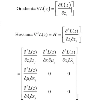
The solution for the OPF problem by Newton’s method requires the creation of the Lagrangian as shown below
( ) T ( ) T ( )L z f x h x g x (15)
inequality constrains. The gradient and hessian of the Lagrangian is then defined as
Gradient=
i L z L z z
(16)and
Hessian=
2
2 ( )
( )
i j
L z L z H
z z
=2 2 2
2 2 ( ) ( ) ( ) ( ) 0 0 ( ) 0 0
i j i j i j
i j
i j
L z L z L z
z z x x
L z x L z x
(17)It can be observed that the structure of the Hessian matrix shown above is extremely sparse. This sparsity is exploited in the solution algorithm. According to optimization theory, the Kuhn-Tucker necessary conditions of optimality can be mentioned as given under,
Let Z*
x*, *, *
, is the optimal solution
* * * *
( ) , , 0
xL z xL x
(18)
* * * *
( ) , , 0
L z L x
(19)
* * * *
( ) , , 0
L z L x
(20)* 0
i
if h x
* 0 (21) (i.e inequality constraint is active)* 0
i
if h x
* 0 (22) (i.e inequality constraint is not active)* 0
i
Real (23)
By solving the equation zL z( )* 0, the solution for the optimal problem can be obtained. Once an understanding of the calculation of the Hessian and Gradient is attained, the solution of the OPF can be achieved by using the Newton’s method algorithm.
IV. PRIMAL LINEAR PROGRAMMING METHOD
Linear Programming (LP) method treats problems having constraints and objective functions formulated in linear form with non negative variables. This method is completely reliable, very fast, accuracy, and adequate for most engineering purposes but has difficulty with marginal losses, to rectify this problem with Primal LP (PLP) OPF solution algorithm. PLP is solving a full ac
power flow solution iteratively, and changes system controls to enforce liberalized constraints while minimizing cost.
The objective function can be written in the following form:
MinimizeF x
o x u, o u
(24) Subjected to g'
xo x u, o u
0 (25)
' o , o 0
h x x u u (26) where xo, uo are the initial values of x and u
x
, u are the shifts about the initial points '
g , h' are the linear approximation to the original and non linear constraints.
The solution of the OPF problem can be achieved by using the primal linear programming in power world simulator.
V. TEST SYSTEMS RESULTS
A. 26 Bus Power System Network
Fig. 1 shows the 26 Bus power system network has been modeled in power world simulator.
Figure 1. 26 Bus power system network model
The generators data and line and bus data of test bus systems have been taken from [4], the generators power production cost and its power generating limits are given in Table I.
TABLE I. GENERATOR’S PRODUCTION COST AND LIMITS
Gen
No. ai bi ci
Min MW Max MW Min. MVAr Max. MVAr
1 240 7.0 0.0070 100 500 0 0
2 200 10 0.0095 50 200 40 250
3 220 8.5 0.0090 80 300 40 150
4 200 11 0.0090 50 150 40 80
5 220 10 0.0080 50 200 40 160
6 190 12 0.0075 50 120 15 50
i
a=Fixed cost,
i
b=Fuel cost,
i
c =Maintenance cost
Bus 1 is reference or slack bus with its voltage
capacitive susceptance are given in per unit on a 100-MVA base. The OPF problem is solved by using Newton and PLP methods.
Figure 2. Comparison voltage between Newton and PLP methods
Fig. 2 shows 26 bus power system network’s voltage profile with Newton and PLP method. The voltage maximum and minimum limits are 1.1 (p.u) and 0.9 (p.u) at each bus in the system. Compared with PLP method, Newton method gives good result to maintain voltage stability problem.
Fig. 3 and Fig. 4 show, the 26 bus power system incremental cost of individual generators and composite generators curves, the system has six generators.
Figure 3. 26 Bus generators incremental cost curves
Figure 4. 26 Bus generators composite incremental cost curve
Fig. 5 shows, 26 bus power systems real power scheduling at each generating bus in the system with Newton method and PLP method to handle the total real power demand 1263 MW.
Figure 5. 26 bus real power scheduling graph with Newton method and PLP method
TABLE II. GENERATORS REAL POWER DISPATCH AND COST OF
GENERATION
Gen. Dispatch Newton Method PLP Method
Gen. No. MW Cost ($/hr) MW Cost ($/hr)
1 447.69 4776.88 457.98 4914.10
2 172.00 2198.04 170 2174.55
3 263.29 3084.97 256 2985.82
4 135.94 1861.73 130 1782.10
5 173.76 2286.02 170 2236.20
6 82.748 1234.33 92 1357.48
Total 1275.40 15441.97 1275.98 15450.24
Table II shows the real power dispatch of each generator and cost of generation with Newton and PLP methods. The total real power generation cost with Primal LP method is 15450.24 $/hr, and the total generation cost with Newton method is 15441.9738 $/hr. Comparing these results, it is seen that there is a savings of 8.2662 $/hr in Newton method. Thus Newton Method gives more economical OPF solution and handles marginal well losses than Primal LP method for OPF calculation.
B. IEEE30 Bus Test Systems
Fig. 6 shows; the IEEE 30Bus power system network has been modeled in power world simulator.
Figure 6. IEEE 30 Bus power system network model
The generators data and line and bus data of test bus systems have been taken from [4], the generators power production cost and its power generating limits are given in Table III. Bus 1 is reference or slack bus with its
impedance and capacitive susceptance are given in per unit on a 100 MVA base. The OPF problem is solved by using Newton and PLP methods.
TABLE III. GENERATOR’S PRODUCTION COST CURVE AND LIMITS
Gen.
No. ai bi ci
Min. MW
Max. MW
Min. MVar
Max. MVar
1 100 2.00 0.00375 50 200 0 0
2 100 1.75 0.00175 20 80 -40 50
3 100 1.00 0.00625 15 50 -40 40
4 100 3.25 0.0083 10 35 -10 40
5 100 3.00 0.0250 10 30 -6 24
6 100 3.00 0.0250 12 50 -6 24
Figure 7. Comparison of IEEE 30 bus voltage profile with Newton method and PLP method
Fig. 7 shows, IEEE 30 bus power system network’s voltage profile with Newton and PLP method. The voltage maximum and minimum limits are 1.1 (p.u) and 0.9 (p.u) at each bus in the system. Compared with PLP method, Newton method gives good result to maintain voltage stability problem.
Figure 8. IEEE 30 bus generators incremental cost curves
Figure 9. IEEE 30 bus generators composite ic curve
Fig. 8 and Fig. 9 show, the IEEE 30 bus power system incremental cost of individual generators and composite generators curves, the system has six generators.
Figure 10. IEEE 30 bus real power scheduling graph with Newton method and PLP method
Fig. 10 shows the IEEE 30 bus test system real power scheduling of each generator in the system with Newton and PLP method to handle the total real power demand 283.40 MW.
TABLE IV. GENERATORS REAL POWER DISPATCH AND COST OF
GENERATION
Gen. Dispatch NR Method PLP Method
Gen. No. MW Cost ($/hr) MW Cost ($/hr)
1 127.98 417.38 128.40 418.61
2 80 251.2 80 251.2
3 50 165.63 50 165.63
4 10 133.33 10 133.33
5 10 132.5 10 132.5
6 12 139.6 12 139.6
Total 289.9 1239.64 290.40 1240.87
Table IV shows the real power dispatch of each generator and cost of generation with Newton method and PLP method. The total real power generation cost with Primal LP method is 1239.64 $/hr, and the total generation cost with Newton method is 1240.87 $/hr. it is seen that there is a savings of 1.23 $/hr in Newton method. It gives more economical OPF solution, voltage stability, and handles marginal losses well than Primal LP method for OPF calculation.
VI. CONCLUTION
The main aim of optimal power flow solution is to minimize the total generating cost of the system while satisfying the load and losses in the system, maximize social welfare, and security of the system. Here the OPF problem is solved by classical methods like Newton method and PLP method. The 26 and IEEE 30 bus systems have been modeled as test bus systems.
ACKNOWLEDGMENT
This work was supported by Dept. of Electrical Engineering, National Institute of Technology Calicut for progress review of Ph.D work in year December 2013.
REFERENCES
[1] H. W. Dommel and W. F. Tinney, “Optimal power flow
solutions,” IEEE Transactions on Power Apparatus and Systems, vol. PAS-87, no. 10, pp. 1866-1876, 1968.
[2] M. Huneault and F. D. Galiana, “A survey of the optimal power flow literature,” IEEE Trans. on Power Systems, vol. 6, no. 2, pp. 762-70, May 1991.
[3] H. Saadat, Power System Analysis, Singapore: WCB/McGraw-Hill,
1999.
[4] D. P. Kothari and I. J. Nagrath, Power System Engineering, 2nd ed. Tata McGraw-Hill Publishers, 2008, pp. 235-389.
[5] J. A. Momoh, R. J. Koessler, and M. S. Bond, “Challenges to optimal power flow,” IEEE Transactions on Power Systems, vol. 12, no. 1, pp. 444-455, Feb. 1997.
[6] H. Kumar and Y. S. Brar, “Optimal power flow using power world
simulator,” in Proc. IEEE Electrical Power and Energy
Conference, 2010, pp. 1-6.
[7] A. Mohammadi and M. H. Varahram, “Online solving of
economic dispatch problem using neural network approach and comparing it with classical method,” in Proc. International Conference on Emerging Technologies, Peshawar, Pakistan, Nov. 2006, pp. 581-586.
[8] W. F. Tinney and C. E. Hart, “Power flow solution by newton’s method,” IEEE Transactions on Power Apparatus and Systems, vol. PAS-86, no. 11, pp. 1449-1460, Nov. 1967.
[9] A. J. Santos and G. R. M. Da Costa, “Optimal power flow solution by newton’s method applied to an augmented lagrangian function,” IEE Proc. Gen. Trans. Distr., vol. 142, no. 1, pp 33-36, 1995.
[10] D. I. Sun, B. Ashley, B. Brewer, A. Hughes, and W. F. Tinney, “Optimal power flow by newton approach,” IEEE Transactions on Power Apparatus and Systems, vol. PAS-103, pp. 2864-2880, Oct. 1984.
[11] S. D. Chen and J. F. Chen, “A new algorithm based on the Newton-Raphson approach for real-time emission dispatch,” Electric Power Syst. Research, vol. 40, pp. 137-141, 1997.
[12] S. Zhang, “Enhanced newton-raphson algorithm for normal
control and optimal power flow solution using column exchange techniques,” IEEE Proc Gen. Trans. Dis., vol. 141, no. 6, 4647-657, 1994.
[13] Y. Y. Hong and C. M. Liao, “Application of newton optimal power flow to assessment of VAR control sequence on voltage security: Case study for a practical power system,” IEE Proc.-C, vol. 140, no. 6, pp. 539-543, 1993.
[14] M. R. Irving and M. J. H. Sterling, “Economic dispatch of active power with constrains relaxation,” IEE Proc.-C, vol. 130, no. 4, 1983.
[15] E. Lobato, et al., “An LP-based optimal power flow for transmission losses and generator reactive margins minimization,” in Proc. IEEE Porto Power Tech Proceedings, Porto, Sep. 2001. [16] T. S. Chung and G. Shaoyun, “A recursive LP-based approach for
optimal capacitor allocation with cost benefit consideration,” Electric Power System Research, vol. 39, pp. 129-136, 1997. [17] R. M. Palomino and V. H. Quintana, “A penalty function linear
programming method for solving power system constrained economic operation problems,” IEEE Trans. on Power Apparatus and Systems, vol. 103, Jun. 1984.
[18] B. Stott and J. L. Marinho, “Linear programming for power system network security applications,” IEEE Trans. on Power Apparatus and Systems, vol. 98, pp. 837-848, 1979.
Guguloth Ramesh is currently Research
Scholar in Electrical Engineering Department, National Institute of Technology, Calicut, Kerala -673601, India. He completed B.Tech (Electrical Engineering) at Christu Jyothi Institute of Technology and Science under JNTU Hyderabad in the year 2008, M.Tech (Power Systems) at National Institute of Technology Calicut (India) in the year 2011. His interested areas in Research are Power Systems, Restructuring Power Systems, Flexible AC Transmission System, and Micro grid.
Dr. T. K.Sunil Kumar, Assistant Professor,
Electrical Engineering Department, NIT Calicut, Kerala-673601, India. He completed B.Tech in Electrical Engineering at N.S.S College of Engineering, Palakkad, M.Tech in Electrical Engineering at NIT Jamshedpur, and Ph.D. from IIT Kharagpur. His interested areas are Model Matching Controller Design Methods with Applications in Electric Power
Systems, Restructuring Power Systems,