Effectively Encoding SAT and Other Intractable Problems into Ising Models for Quantum Computing

(1)

Effectively Encoding SAT and

Introduction

Disclaimer: The research work described in this PhD Dissertation is joint work with Dr. Zhengbing Bian, Dr.Fabian Chudak, Dr.William Macready, Dr.Aidan Roy from D-Wave System Inc. and with my advisor Prof.Roberto Sebastiani from Universit`a di Trento. Most of the scientific content pre-sented here can be found in the papers:

• Zhengbing Bian, Fabian Chudak, William Macready, Aidan Roy, Roberto Sebastiani, and Stefano Varotti. Solving SAT and MaxSAT with a quantum annealer: Foundations and a preliminary report. In The 11th International Symposium on Frontiers of Combining Sys-tems, FroCoS’17, volume 10483 of LNCS. Springer, 2017.

• Zhengbing Bian, Fabi´an A. Chudak, William G. Macready, Aidan Roy, Roberto Sebastiani, and Stefano Varotti. Solving SAT and MaxSAT with a quantum annealer: Foundations, encodings, and preliminary results. 2018. https://arxiv.org/abs/1811.02524 . Under submis-sion for journal publication.

(16)

weird-1.1. THE PROBLEM CHAPTER 1. INTRODUCTION

ness to obtain computational speedups, but the development of quantum computing hardware has been stuck by the high susceptibility to noise. While noise tolerant quantum circuits are slowly improving over time, the currently available hardware shows a behavior that is typical of quantum systems but provides limited computational flexibility. Quantum anneal-ers accept some level of noise and decoherence to allow for large quantum systems.

1.1

The Problem

Quantum annealers are able to solve a specific subset of a single optimiza-tion problem. Whereas this problem is NP-hard, and thus it is theoretically possible to convert any NP problem instance into such problem, in practice the process of encoding is difficult due to several limitations.

The thesis will focus on SAT problems, as alternative tools able to tackle worst-case instances would be critically useful. Whereas the hardware is able to solve several NP-hard problems it is not particularly suited to solve SAT problems. To demonstrate the capabilities of quantum annealing, SAT problems that are considerably hard for state-of-the-art SAT solvers are preferred. Encoding such a problem into a quantum annealing problem would provide a convincing evaluation for the approach.

1.2

The Solution

(17)

solving is instead used to build a library of efficiently encoded gates. The second part of the solution consists in a multi-step process where the input Boolean formula is broken into multiple components from the pre-encoded library and these elements are re-composed into a final quantum annealing problem. This part uses a heuristic approach to shape the input formula into an encoding that respects the hardware constraints.

This approach provides an effective and efficient method for SAT prob-lem encoding. It is thought for SAT solving of generic Boolean circuits, while the state of the art is focused either on optimization problem or in specific constraint satisfaction problems.

1.3

Structure of the Thesis

The first half of the thesis, containing Chapter 2 to 4, will provide the context and background for the thesis. The second chapter will outline the motivations behind this area of research and the goals of this thesis, why quantum computing can be useful and what are the current limits. The third chapter will provide a comprehensive background on quantum computing, quantum annealing and other aspects of quantum computation, and then it will introduce various logic problems such as SAT, MaxSAT, SMT and OMT. The fourth chapter will survey related work on the same problem and highlight differences and limitations.

(18)

1.3. STRUCTURE OF THE THESIS CHAPTER 1. INTRODUCTION

(19)

Motivations, Background,

(20)

(21)

Motivations and Goals

Quantum computing research has been thriving over the last decades since its inception. This chapter is dedicated to explaining the reason for this interest, what is its potential advantage over currently available computers, and what are the obstacles that need to be overcome. First it will introduce the context of quantum computation and computational complexity. Then it will outline the computational advantages of quantum computing, and its practical limits. Finally, the chapter will focus on the particular branch that the thesis will contribute to and on which are the main obstacles to be overcome.

To understand the interest in quantum computing we need to consider its context in the field of complexity theory. Complexity theory is con-cerned with the asymptotic resource requirements necessary to solve a problem. One of the most important results in complexity theory is NP-completeness and NP-hardness. These concepts are fundamental and re-quired for understanding quantum computing. In the last 20-30 years there has been a development of the theory of quantum computing complexity. This theory has important implications in computer science and physics and opens new possibilities in computing.

(22)

2.1. INTRACTABLE PROBLEMS CHAPTER 2. MOTIVATIONS

reached the goal of manufacturing reliable large-scale devices, limited alter-native models have proven to be feasible. In particular, quantum annealing has shown an advantage over the classical version, simulated annealing. We will see how quantum annealing differs from gate-model quantum comput-ers and what are the limits of this approach.

2.1

Intractable problems and NP-Hardness

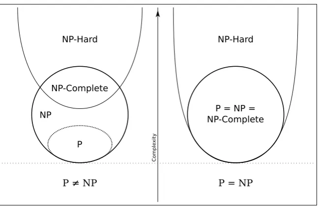
Two of the most important concepts in complexity theory are nondeter-ministic polynomial complexity and NP-hardness. The Nondeterminis-tic Polynomial (NP) class of problems consists in all the problems that have an algorithm that, given a solution, are able to check it in polynomial time. If no better algorithm is available, in the worst case every possible solution has to be checked. A NP-hard problem is a problem such that an instance of any problem in the NP class can be converted into an instance of the NP-hard problem. Thus, an efficient solver for any single NP-Hard problem would be capable to solve all NP problems as well. For this reason NP and NP-hard problems are considered to be intractable, i.e. they do not have an efficient algorithm. The proof of intractability of NP problems (the so-called P vs. N P problem) is still an open problem, but intractability is strongly believed due to various weaker theorems [46]. All NP-complete and NP-hard problems known so far have no efficient algorithm, and any algorithm found would solve efficiently all the other problems. When we encounter NP-hard algorithms in the real world, we rely on heuristics and approximations, and we are not guaranteed to reach the solution of our problem in a reasonable time.

(23)

Comple

xity

P ≠ NP P = NP

NP-Hard

NP-Complete

P NP

NP-Hard

P = NP = NP-Complete

Figure 2.1: Venn diagrams for complexity classes, ifP 6= N P or if P =N P. cBehnam Esfahbod, under CC-BY-SA license.

on the intractability of various NP algorithms. As an example that will be useful later, Public Key Cryptography relies on the hardness of the factorization problem. Factorization is in NP and no polynomial time algorithm is known, but it is not believed to be NP-hard. The abstract nature of the NP-hardness definition implies that problem complexity and intractability is independent of the hardware used, as long as it follows the deterministic turing machine model. This was the case for all known computer architectures until the development of quantum computing the-ory. The non-determinism of quantum mechanics happens to allow a more powerful model of computation.

2.2

Quantum efficient problems

(24)

2.2. QUANTUM EFFICIENT PROBLEMS CHAPTER 2. MOTIVATIONS

are intrinsically unknowable. It is an inherently probabilistic theory, un-like statistical mechanics. In the classical statistical mechanics view of the world, probability distribution is caused by the uncertainty of the observer. In quantum mechanics we have superposition of states instead. Different world histories interfere with each other. This leads to all kinds of counter-intuitive phenomena: entanglement, tunneling. A notable example is the Einstein-Podoslky-Rosen paradox, an experiment that disproves any hid-den variable theory [86].

Quantum computing is a model of computation that relies on the weird-ness of quantum mechanics. We expect a computer to strictly follow a specific sequence of instructions and acts on it internal state to reach a so-lution. This is the deterministic model of computation. Non-deterministic automata instructions instead are partially defined, and succeed when there exists a sequence of legal instructions that solve the problem.

(25)

Problem Classical complexity

Quantum

complexity Quantum speedup Factorization O(e(nlogn)1/3) O(n2logn) exponential Unstructured search O(2n₎ ₂√n _quadratic Deutsch–Jozsa algorithm O(2n) 1 exponential

Table 2.1: Complexity comparison between various algorithms, quantum speedups [56]. computing subsumes classical computing so it can only improve.

The most famous problem that is sped up by quantum computers is fac-torization, which hardness underlies all public key cryptography schemes used nowadays on the Internet. In 1994, Peter Shor showed that there is a quantum algorithm that solves efficiently factorization[87]. Thus the abil-ity to manufacture a scalable quantum computer would compromise most current internet security standard. As research makes quantum computing more and more feasible, there is large interest for quantum-proof encryp-tion, and work for standardization is underway[11, 26]. On the upside, another important problem in BQP is simulation of quantum systems[40]. Quantum supremacy obviously implies that quantum systems are not ef-ficiently simulable by classical computers. We would like to predict and analyze the behavior of quantum systems, and classical computer can do so with limited accuracy. An efficient quantum simulation would be extremely useful in science, especially material science.

Still, a quantum computer is not as powerful as a generic non-deterministic Turing machine. Grover’s algorithm [51] provides a brute-force search that improves worst case complexity from O(2n) to O(2

√

n_{), and} subse-quent work has proved that this is the best possible quantum algorithm for unstructured search[10]. In this case then the best result we can get is only a quadratic speedup, which is still worse than a non-deterministic Turing machine that is exponentially faster.

(26)

2.3. NOISE & QUANTUM COMPUTING CHAPTER 2. MOTIVATIONS

can be obtained only when the problem has an underlying structure that can be exploited. For example, factorization can be sped up because it is a special case of the so-called subgroup problem. The hidden-subgroup problem consists in finding an algebraic group hidden in a bigger algebraic structure, and quantum computers can solve it efficiently in the case of finite Abelian groups. Table 2.1 shows a sample of algorithms and their best-known complexities on classical and quantum computers.

2.3

Noise and decoherence in quantum computing

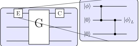
Whereas quantum computing theory has grown considerably and presented many useful novel algorithms, the construction of an actual quantum com-puter has proved to be a challenge. As we will see later, quantum comput-ing assumes a noiseless computcomput-ing hardware, and by itself has no provision for noise tolerance. Thus, quantum computers are really sensitive to noise, as any interaction with environment causes decoherence. A system that fully loses coherence becomes equivalent to a non-quantum system in a random state. Indeed a topic of great interest in quantum computing and quantum communication is error resilience. Some solutions are quantum error correction or topological quantum computing.

E C

G

|φi |0i |0i

|φi_L

Figure 2.2: An example of quantum circuit, where the input is encoded. Each logical qubit is represented as group of three physical qubits (on the right), and is error corrected after the operation.

(27)

in order to be able to cope with corruption of quantum states. A system of multiple qubits is used to resiliently store a single logical qubit. An illus-tration of a circuit with a simple error correction mechanism is available in Figure 2.2. Before the computation happens, a single logical qubit is encoded into multiple qubits and after computation any error or change is corrected. If the error level in the underlying system is below a certain threshold, one can build a error correction system with arbitrarily low error rate[47]. It is estimated that thousands of qubits are necessary for error-correcting a single logical qubit[27]. Whereas the technology is bound to improve, error-free quantum computation needs to attain significant man-ufacturing improvements before being possibly realizable.

(28)

2.4. AQC AND ANNEALING CHAPTER 2. MOTIVATIONS

2.4

Adiabatic Quantum Computing and Quantum

An-nealing

Quantum annealing is closely related with the theory of adiabatic quantum computing. Adiabatic quantum computing is an alternative model of quantum computing that exploits the quantum adiabatic theorem. This theorem ensures that a quantum system that evolves sufficiently slowly in time will stay in the lowest energy state, called ground state. An adi-abatic quantum computer works by slowly transitioning a cold quantum system from a standard initial state into a desired final state. The user programs the computer by engineering the system in such a way that its final ground state encodes the solution to the specified problem. The time necessary to perform this transition is determined using the quantum adi-abatic theorem, and depends on the lowest energy gap between the ground state and the second lowest energy state during the transition.

(29)

error correction threshold theorem for AQC.

Adiabatic quantum computing assumes that the system never leaves the ground state. This happens only when the system is at absolute zero and perfectly isolated, or at least when it is isolated up to noise lower than the minimum gap. In real systems though the temperature can never reach absolute zero, and noise cannot be eliminated completely. Thus with the current technology we cannot reliably ensure the adiabatic condition. In fact, current hardware still faces significant problems in managing noise and large scale systems tend to lose coherence very fast.

We can still exploit the fact that when the adiabatic condition is re-moved the system still tends toward the lowest energy state in a process called annealing. A quantum annealer still shows the presence of quantum effects but loses coherence during the run. Quantum annealing accepts a loss of coherence that is too big to perform adiabatic quantum computing, but still manages to exploit partial coherence to perform tunneling. While simulated annealing perform a stochastic search of the lowest energy state, a quantum annealer tries to exploit coherence to explore a larger state space at the same time [4].

Quantum annealers, compared to the quantum gates model, have also a benefit in their affinity to the simulated annealing algorithm. While quantum algorithm like Shor’s algorithm have no counterpart in classical computing, simulated annealing is a widely used and established algorithm in stochastic optimization. Thus simulated annealing can provide a clear reference for evaluating performance and results of quantum annealers.

2.5

Quantum Annealers and D-Wave

(30)

2.5. D-WAVE QA CHAPTER 2. MOTIVATIONS

(31)

(32)

2.5. D-WAVE QA CHAPTER 2. MOTIVATIONS

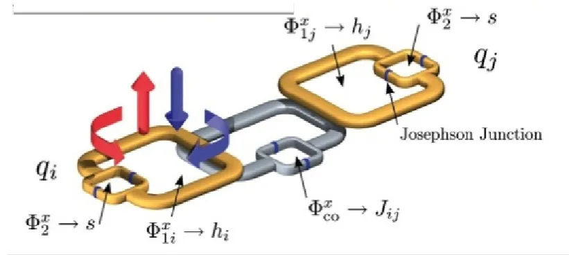
The energy model of a D-Wave quantum annealer can be represented by a second degree real polynomial in where qubit states can be either -1 or 1. Such type of models is widely studied in Physics, and it is known as Ising model. The formula for this model is shown in equation 2.1. In this model, z_i are variables in {−1, 1} and represent the state of a qubit. The parameters θ that influence the system’s behavior are divided in three types: θ₀ is called offset, the θ_i are called biases and the θ_ij are called

couplings.

P(z) =def θ₀ +X i

θ_iz_i +X i,j

θ_ijz_iz_j (2.1)

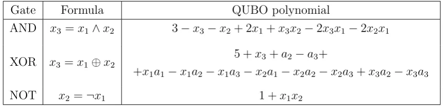
The problem of finding the ground state given of an Ising model is a particular case of the so called quadratic unconstrained binary opti-mization (QUBO) problem.1It is easy to show that QUBO is a NP-hard problem by reducing CIRCUIT-SAT (satisfiability of a Boolean circuit), a NP-complete problem, into QUBO. We can translate each gate of a cir-cuit into a simple sub-problem and then compose them in a consistent way (we will see later how). Table 2.2 shows simple translations for basic logic gates.

Gate Formula QUBO polynomial

AND x3 =x1∧x2 3−x3−x2+ 2x1+x3x2 −2x3x1−2x2x1

XOR x3 =x1⊕x2

5 +x3+a2−a3+

+x1a1−x1a2−x1a3−x2a1−x2a2−x2a3+x3a2−x3a3

NOT x2 =¬x1 1 +x1x2

Table 2.2: QUBO encoding of the basic logic gates. The QUBO polynomial is at its minimum value when the relation between variables is true. Notice how implementing the XOR gate requires adding two ancillary variables.

1_{Usually QUBO problems are stated on variables in}_{₀_,₁_}_{rather than}_{−₁_,₁_}_{, which is an equivalent}

(33)

D-Wave’s machine has been demonstrated to have better performance than simulated annealing for certain random QUBO problems [59], and has been used for solving traffic optimization [73] and quantum simula-tion of material properties [57]. Using the naive conversion from SAT to QUBO instead yields QUBO problems that are not suited to the annealer architecture, thus so far naively-encoded circuits are too large or are very simple for a traditional SAT solver.

(34)

2.6. ENCODING ISSUES CHAPTER 2. MOTIVATIONS

2.6

Issues in Encoding for Quantum Annealers

Quantum annealers are still hard to build and operate at large scale. While naive conversion from circuit to QUBO is straightforward, the result is cannot be passed to the quantum annealer directly. This is because so far:

• The number of available qubits is limited. • The number of couplings is limited.

• Noise and control precision limit the chances of success.

The number of available qubits is limited. Even with 2000+ qubits, the size of problems that can be solved is still small. This is because the majority of qubits in quantum annealing has to be used to encode the problem, unlike circuit models where the number of qubits represent the input width and the circuit size are two different metrics for complexity. Consider a boolean circuit that we want to check for satisfiability. In Grover search we need enough gate to set up a superposition and run the circuit reversibly, and while this is costly we can reuse qubits for intermediate values. When using quantum annealing we need to encode the full circuit into a Ising model. Thus a deep circuit using many levels with relatively few bits at a time (for example, a cryptography primitive with a limited internal state and many computation rounds) will require less qubits (ignoring the space requirements of gates).

(35)

root of the number of qubits. The problem encoding process then has to accommodate for the couplings that are available. In general, there is a measure that correlates directly with problem complexity[39], called tree-width. It is a measure of similarity to trees and will play an important role in the encoding process. In Chimera and Pegasus, tree-width grows linearly with the number of qubits.

(36)

2.7. GOALS CHAPTER 2. MOTIVATIONS

Noise and control precision limit the chances of success. Whereas the D-wave machine is close to 0 K and heavily shielded, noise can still cause performance degradation. In annealing the ground state of the annealer encodes the best solution of our problem while higher energy states are less useful. Thus we wish to have energy gaps between solution and non-solutions that are as large as possible. Furthermore, obviously there are range bounds and precision limits on the biases and couplings.

2.7

Goals

The concept of intrinsic greater power of quantum computers is generally called quantum supremacy. Proving quantum supremacy with a real device is a major goal of quantum computing research. To test for it we need problems that are impossible for standard computers and easy for quantum ones. CSP and SAT problems are very general problems, and tend to become very hard even for small sizes. SAT problems have the potential to be small enough to fit in the hardware but are still very hard for traditional computers.

D-Wave’s quantum annealers have proven their strength for certain rdom QUBO problems that match their architecture. Exploiting the an-nealer for generic problems is less straightforward due to the need of en-coding. Quantum annealing hardware is expected to grow in a Moore-like fashion, so it will eventually reduce the overhead, but we want to exploit in the best way the hardware we have now or in the near future, and possibly to solve interesting problems with it. My research goal is to pick a NP-hard problem and convert into an Ising problem in an effective and efficient way.

(37)

considerably big/difficult.

Efficient means that the encoding process is reasonably fast to perform, at least it has to be faster than actually trying to solve the problem with a standard computer.

(38)

(39)

Background

3.1

Quantum computing

We will start with a quick survey on quantum computing. Whereas the en-coding process can consider the actual computation as a black box process, the theory behind quantum computation is useful to justify the context of the thesis and it can provide useful tools to interpret the results. As the survey will be lacking in depth, the reader is invited to refer to Quantum Computation and Quantum Information[74] for further details.

3.1.1 Quantum mechanics

The theory of quantum mechanics is based on the theory of complex linear algebra. In this survey a basic knowledge of linear algebra will be neces-sary, but most of the concepts will be explained as they appear. For the purpose of the thesis the survey will assume only the finite dimensional spaces, as they represent quantum system with discrete states. General-izing results from finite-dimensional to infinite-dimensional spaces is not trivial, but most of the assertions in this survey are equally valid in the infinite-dimensional case.

(40)

3.1. QUANTUM COMPUTING CHAPTER 3. BACKGROUND

basic postulates. These postulates will serve as a framework to write and reason about quantum phenomena. The first postulate defines the state of a quantum system:

Postulate 1. Associated to any isolated physical system is a complex vector space with inner product (that is, a Hilbert space) known as the state space of the system. The system is completely described by its state vector, which is a unit vector in the system’s state space.

The basis of the Hilbert space will represent the set of possible out-comes, i.e. the post-measurement classical states that we can observe. For example, a system with two possible states (i.e. a qubit), the state of the system will be represented as a two dimensional vector with two basis vec-tor that we will call, using the ket-notation, |0i and |1i. We call a pure state a unit vector (or, equivalently, a ray) in the Hilbert space that rep-resents a possible state of the system. We consider only unit vectors as states as possible outcomes depend only on the relative amplitudes and phases between vector components.

A pure state represents a perfectly known system; We can model uncer-tainty over the quantum state with the so-called mixed states. A mixed state is a distribution over superposition of states. It can be represented simply as a density operator, a convex combination of multiple projective operators. Thus, given possible states |Ψ_ii with probabilities p_i, the mixed state ρ of the system is:

ρ = X i

p_i|Ψ_ii hΨ_i| (3.1) Two observations can be done on this formula. First, the density matrix for a pure state is simply its projection operator |Ψi hΨ|. Then, in the same way that P

(41)

The second postulate describes how a quantum system evolves over time:

Postulate 2. The time evolution of the state of a closed quantum system is described by the Schr¨odinger equation,

id|Ψi

dt = H |Ψi (3.2)

H is a fixed Hermitian operator known as the Hamiltonian of the closed system. Then, the evolution of a closed quantum system is described by a unitary transformation. That is, the state |Ψ₁i of the system at time t₁ is related to the state |Ψ₂i of the system at time t₂ by a unitary operator U which depends only on the times t1 and t2.

|Ψ₂i = U |Ψ₁i (3.3) Recall that an Hermitian operator is an operator H that is its own dual (H = H†) and always has a spectral decomposition (H = P

iei|Eii hEi|, ei ∈

R), while a unitary operator is a operator U such that U†U = I. The

spectral decomposition of the Hermitian matrix in Schr¨odinger equation has an important interpretation. The eigenstates |E_ii are called station-ary states, and the eigenstate with lowest eigenvalue e₀ is called ground state. A direct consequence of the spectral decomposition is that quantum states evolve using unitary matrixes. If the quantum state is a unit vector, a quantum computer instruction is a unitary operator.

We can easily generalize system evolution on a mixed state ρ given the unitary operator U:

ρ0 = U ρU† (3.4)

(42)

3.1. QUANTUM COMPUTING CHAPTER 3. BACKGROUND

Hamiltonian. For many such systems we can write a time-varying Hamil-tonian, where the effect of the environment on the system is represented with a changing Hamiltonian H(t):

id|Ψi

dt = H(t)|Ψi (3.5)

The third postulate describes how the quantum world interacts with the classical world, i.e. how measurements are made.

Postulate 3. Quantum measurements are described by a collection {M_m} of measurement operators such that:

X

m

M_m†M_m = I (3.6)

These are operators acting on the state space of the system being mea-sured. The index m refers to the measurement outcomes that may occur in the experiment. If the state of the quantum system is |Ψi immediately before the measurement then the probability that result m occurs and the state of the system after the measurement are given by:

p(m) =hΨ|M_m†M_m|Ψi (3.7) |Ψ_mi = √Mm|Ψi

p(m) (3.8)

The postulate is the most general specification of measurement. In the simplest case, called projective measurement, the M_m operators can be mapped into projective operators for a particular basis of the Hilbert space:

(43)

This form allows us to represent concisely the expected value of the mea-surement _E_Ψ[M].:

M = P

mm|φmi hφm| (3.10)

EΨ[M] = hΨ|MΨi (3.11)

We can generalize the measurement of a mixed state ρ and get its prob-ability and post-measurement state:

p(m) = tr(M_m†M_mρ) (3.12)

ρ_m = M

†

mρMm

p(m) (3.13)

Notice how we have non-determinism in measurement. Even in a fully-known pure state the outcome of a measurement can be random. Fur-thermore, measurement is a destructive operation, as the original state is modified, and only projective measurements are repeatable, i.e. applying the same measurement twice yields the same result.

The last postulate describes the composition of quantum states:

Postulate 4. The state space of a composite physical system is the tensor product of the state spaces of the component physical systems. Moreover, if we have systems numbered 1 through n, and system number i is prepared in the state |Ψ_ii, then the joint state of the total system is |Ψ₁i ⊗ |Ψ₂i ⊗

...⊕ |Ψ_ni.

(44)

3.1. QUANTUM COMPUTING CHAPTER 3. BACKGROUND

|0_ai ⊗ |0_bi = |00i |0_ai ⊗ |1_bi = |01i |1_ai ⊗ |0_bi = |10i |1_ai ⊗ |1_bi = |11i

It follows then that the number dimensions of a discrete Hilbert space doubles for each added qubit. Thus, the representation of a quantum state in a classical computer needs an amount of space that is exponential to the number of qubits. This is one of the reasons for distinction from quantum and classical computing, and what makes many-body matter simulations hard to simulate and predict.

Another important consequence is that a two-qubit system can be put in entangled state |Ψi = |00i + |11i. This state is peculiar because the system cannot be expressed anymore as the composition of two single-qubit systems: this is an entangled state.

3.1.2 Qubits, quantum gates, adiabatic computing

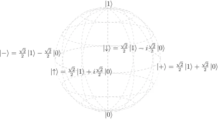
The basic unit of quantum information is a qubit, a discrete quantum system with two possible states usually called |0i and |1i. While a bit is an element that can be in one of two states, a qubit is in a superposition of these two states. A qubit state can be represented as a point on the Bloch sphere. A pure state is a point on the surface while a mixed state as a point inside its volume. Notice that this representation fails to generalize to multiple qubits.

(45)

|1i

|0i

|+i=

√ 2 2 |1i+

√ 2 2 |0i |−i=

√ 2 2 |1i −

√ 2 2 |0i

|↑i=

√ 2

2 |1i+i √

2 2 |0i

|↓i=

√ 2

2 |1i −i √

2 2 |0i

Figure 3.1: Representation of the state of a single qubit as a Bloch sphere. Any point on the surface of the sphere represents a pure state, and any point inside the sphere represents a mixed state.

is negation (Equation 3.14), other important operations are the Hadamard gate (Equation 3.15) and the π/8 half-phase gate (Equation 3.16).

X = " 0 1 1 0 # (3.14) H = √ 2 2 " 1 1 1 −1 # (3.15) T = " 1 0 0 eiπ/4

#

(3.16)

(46)

funda-3.2. AQC ANDQA CHAPTER 3. BACKGROUND

mental for quantum computing theory, and by virtue of their universality they can represent any computation done by quantum systems, but as we will focus on quantum annealing, they will be of limited use.

X H T

Figure 3.2: Standard representation for the basic quantum gates (from left to right: negation, Hadamard, half-phase and controlled not).

3.2

Adiabatic Quantum Computing and quantum

an-nealing

3.2.1 Adiabatic Quantum Computing

The adiabatic quantum computing approach relies on the adiabatic quan-tum theorem. It is a direct consequence of the time-dependent Shr¨odinger equation. The adiabatic theorem states that when the Hamiltonian changes slowly enough over time, a quantum system that starts in the initial ground state ends in the final ground state.

Theorem 1. Given a quantum system at ground state Ψi₀

and the time-varying Hamiltonian H(t) =H_i(T−t) +H_ft, given large enough transition time T the system will stay in the ground state up to the final state

Ψ

f

0

E . As stated above, the theorem does not specify any explicit bound on

(47)

operator that can be approximated by quantum gates. The reader that is interested in a thorough exposition is suggested to consult [3].

The quantum adiabatic theorem holds for a system that is already at the ground state. If we switch point of view to thermodynamics, this state is at the absolute zero temperature. In theory, in an adiabatic quantum system the quantized energy gaps theoretically ensures that a higher temperature requires a discrete amount of energy. In thermodynamics when the tem-perature is not zero we have a process called annealing. Both in classical and quantum annealing the probability of a certain state is governed by Boltzmann statistics, stated in Theorem 2.

Theorem 2. A thermodynamic system at equilibrium can be found in the state x with the following probability:

p(x) = 1

Ze

E(x)

kT (3.17)

where T is the temperature of the system, and Z is the partition function:

Z = P xe

E(x)

kT

The Boltzmann distribution is used widely to calculate properties of thermodynamics systems. The most relevant observation for the thesis is that when the temperature is high every state is equi-probable while when the temperature is small low energy states are more probable. Simulated annealing consists essentially in simulating a system moving toward equi-librium while lowering the temperature. A low energy state consists in a solution with a low cost according to the problem constraints.

(48)

3.2. AQC AND QA CHAPTER 3. BACKGROUND

3.2.2 Ising models

So far the Hamiltonian function that represent the energy landscape has been not yet defined. The quantum annealers that will be used in this thesis will have an Ising energy model. The Ising model is one of the most important models in statistical physics. It has been used to study various phenomena in matter, like magnetization.

In the Ising model the particles/elements can be only in two states, −1 or 1. The Hamiltonian is defined as a second degree real polynomial on binary variables (Equation 3.18). In this polynomial θ_i represent biases of a single element, while θ_ij represent the effect of interaction between pairs of elements.

H(z) = X i

θ_iz_i+ X ij

θ_ijz_iz_j (3.18)

The problem of finding the minimum of a polynomial over binary vari-ables is called quadratic unbounded binary optimization (QUBO). A QUBO problem ask, given a quadratic polynomial with binary variables what is its minimum value assignment. In the QUBO literature it is usually assumed that variables takes values in {0,1} while Ising model variables take values in {−1,1}, but the two representations are equivalent and con-version is trivial. If the state of the system is expressed as a binary vector

z ∈ {0,1}n, the QUBO problem derived by an Ising model can be expressed also as a quadratic form (Equation 3.19). In this case the parameters are represented with a single matrix Θ.

(49)

3.2.3 Induced graphs and their properties

Ising models are generally classified by the topology of the interaction. Given a second degree polynomial we can define aninduced graph where vertices are variables/qubits, edges are non-zero second degree terms or available couplings. The properties of the induced graph are important in terms of complexity of the problem and useful for encoding. Given a graph G, a graph minor is a graph where an edge or a vertex is removed, or two vertices are merged. When G is an induced graph, setting the value of a variable or forcing equivalence between two variables is equivalent to removing or merging vertices.

The shape of the induced graph of a QUBO problem affects its hardness. We have seen that QUBO is a NP-hard problem in the general case, but it is not trivial that an Ising model with a certain topology is NP-Hard as well, and indeed a planar graph with no biases are tractable [7]. Later we will see various method to reduce general QUBO problems into problems that have the induced graph of the quantum annealer hardware.

In later chapters we will make use of symmetries in induced graphs. A permutation σ : V → V is an automorphism of a graph G if relabeling its vertices with σ produces the same graph: σ(G) = G. Automorphisms form a group (where the identity function is the identity and function composition is the operator), called Aut(G). When the group is associated with an action φ(σ, x) : (Aut(G), X)− > X (see [43]) the group orbit of x

is the set of elements of X that can be reached from x: G×x = {∀g ∈

Aut(G) : φ(g, x)}. Group orbits form a partition of X, and thus form an equivalence relation on it.

Another important graph property is tree-width. The tree-width en-codes the smallest node clustering that yields a tree. Given a graph

(50)

3.2. AQC AND QA CHAPTER 3. BACKGROUND

such that:

• X₁, ..., X_n are subsets of V_G, and S

X_i = V_G.

• All the X_i that contains a vertex v form a connected subtree of T. • For every edge (v, w) ∈ E_G there exists a X_i that contains both v and

w.

The width of the decomposition is the maximum size of the X_i minus 1, and the tree-width of a graph is the minimum width for all possible decompositions of a graph. Figure 3.3 illustrates a simple tree decomposi-tion of width 2. Tree-width is an important property in computer science: the complexity of a dynamic programming depends on the tree-width of the problem dependencies, and CIRCUIT-SAT complexity is linear for a circuit of fixed tree-width. Tree-width is NP-Hard to compute but is easy to approximate using heuristics methods.

3.2.4 D-Wave machine

(51)

A

B

A

C

B

D

E

F

G

H

(52)

3.2. AQC AND QA CHAPTER 3. BACKGROUND

Figure 3.4: Illustration of a SQUID qubit. The user sets the various biaseshiand couplings

Jij by tuning the various magnetic fields Φ.. Courtesy of D-Wave Systems Inc.

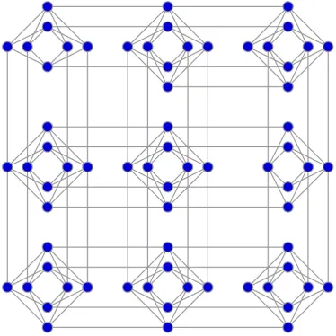
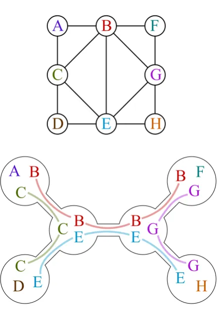
The latest annealer is called D-Wave 2000Q, announced in 2017. Since October 2018 is available to the public through a cloud service.1 The D-Wave 2000Q machine has 2048 qubits and 5600 couplers in a regular pattern called Chimera topology. This topology consists in groups of 8 tightly connected qubits in a bipartite graph called cell, and a grid of cells where 4 qubits have vertical parallel connections and 4 qubits have horizontal parallel connections. Figure 3.5 shows the induced graph of a D-Wave 2000Q Chimera chip.

The Chimera topology is a bipartite graph, thus there are no cliques. This topology contains as a minor complete graphs and complete bipar-tite graphs, we will see then how to encode complete graphs into chimera topology. Thanks to the cell separation encoded problems often have a clear cut distinction between functional units, where complex relationship are expressed using the dense connection within the chip and couplings between cells are used to transfer information.

While all the published work so far has been on the Chimera

(53)

ogy, in 2018 D-Wave divulged details about a newer topology, the so called

(54)

3.2. AQC AND QA CHAPTER 3. BACKGROUND

(55)

(56)

3.3. SAT, MAXSAT, SMT AND OMT CHAPTER 3. BACKGROUND

3.3

SAT, MaxSAT, SMT and OMT

3.3.1 Basics

In the following we recall the main concepts of the basic syntax, semantics and properties of Boolean and first-order logic and theories. We refer the reader to [19, 65, 62, 9, 84] for more details.

Boolean logic deals with formulas over Boolean variables, variables that can assume the value true (>) or false (⊥). Given some finite set of Boolean variables, or Boolean atoms, x the language of Boolean logic (B) is the set of formulas containing the atoms in x and closed under the standard propositional connectives {¬,∧,∨,→,↔,⊕} (respectively called: NOT, AND, OR, IMPLY, IFF, XOR).

The AND (∧) operation is also called conjunction, OR (∨) is also called disjunction and NOT (¬) is also called negation. All other con-nectives can be defined in terms of disjunction, conjunction and negation. The meaning of these connectives, i.e. the value of the formula given the value of its variables, can be defined using truth tables. A literal is an atom, x (positive literal) or its negation ¬x (negative literal). We implic-itly remove double negations: e.g., if l is the negative literal ¬x_i, then by ¬l we mean x_i rather than ¬¬x_i.

A formula is in negative normal form (NNF) if only AND and OR are used, and negation appears only in negative literals. Every formula can be converted into NNF using deMorgan’s theorems. A clause is a disjunc-tion of literals. A formula is in conjunctive normal form (CNF) if it is written as a conjunction of clauses. Conversely, a cube is a disjunction of literals and a formula is in disjunctive normal form (DNF) if it is written as a disjunction of cubes.

An assignment x satisfies F(x) iff it makes it evaluate to true. If so,

(57)

one truth assignment satisfies it, unsatisfiable otherwise. F(x) is valid

iff all truth assignments satisfy it. F₁(x), F₂(x) are equivalent iff they are satisfied by exactly the same truth assignments.

A formula F(x) which is not a conjunction can always be decomposed into a conjunction of smaller formulas F∗(x,y) by means of Tseitin’s transformation [94], as in Equation 3.20, where the F_is are simple sub-formulas which decompose the original formula F(x), and the y_is are fresh Boolean variables each labeling the corresponding F_i.

F(x) = F_m(F_m−1(...(F1(x))))

F∗(x,y) =def Vm_i₌₁−1(y_i ↔F_i(xi,yi))∧ F_m(xm,ym) (3.20) Tseitin’s transformation guarantees that F(x) is satisfiable if and only if F∗(x,y) is satisfiable, and that if x,y is a model for F∗(x,y), then x is a model for F(x). For this reason it is used recursively for efficient CNF conversion of formulas [94].

Aquantified Boolean formula (QBF)is an extension over the afore-mentioned Boolean formulas. It is defined inductively as follows: a Boolean formula is a QBF; if F(x) is a QBF, then ∀x_iF(x) and ∃x_iF(x) are QBFs. QBFs can be converted to Boolean formula through Shannon’s expan-sion: ∀x_iF(x) is equivalent to (F(x)_x_i₌>∧F(x)xi=⊥) and∃xiF(x) is

equiv-alent to (F(x)_x_i₌> ∨F(x)xi=⊥).

3.3.2 And-Inverter Graphs

(58)

3.3. SAT, MAXSAT, SMT AND OMT CHAPTER 3. BACKGROUND

1. Each x_i has no incoming edges and each g_k has 2 incoming edges, and there is a unique g_o with no outgoing arcs (the primary output). 2. Each edge z →g is labelled with a sign + or − indicating whether or

not z should be negated as an input to g; define a literal l_i(z) =z for an edge with sign + and l_i(z) =¬z for an edge with sign −.

3. For each node g_k with edges incoming from z₁ andz₂, there is an AND function A_k(g_k, z₁, z₂) = g_k ↔l_k(z₁)∧ l_k(z₂), such that

F(x) ↔ m ^

k=1

A_k(z)∧(g_o = >). (3.21)

If is F(x) is in CNF form, we can trivially construct an AIG by rewriting each OR clause as an AND function using De Morgan’s Law, and then rewriting each AND function with more than 2 inputs as a sequence of 2-input AND functions.

Example 1. The function

F(x) =x₁ ∧x₂ ∧ ¬x₃

is represented by both of the And-Inverter Graphs in Figure 3.7.

x1 a1 x2 a2 x3 ao + + + -+ + x1 a1 x2 x3 ao + + +

-Figure 3.7: Two And-Inverter Graphs representing the functionF(x) = x1∧x2∧ ¬x3.

Let G be an AIG with a node z. A cut C of z is a subset of vertices of

G such that every directed path from an input x_i to z must pass through

(59)

path from C to z is effectively a AIG representation of z as a function of C, since the Boolean value of z is determined completely by C. The equivalent function is the Boolean function of z represented by C. Cut C is k-feasible if |C| ≤ k and non-trivial if C 6= {z}. For fixed k, there is a simple linear-time algorithm to enumerate all k-feasible cuts in an AIG. Starting from the inputs x to the primary output, we can traverse the graph to list the k-feasible cuts of node a_i by combining k-feasible cuts of a_i’s two inputs.

3.3.3 SAT

Propositional Satisfiability (SAT)is the problem of establishing whether an input Boolean formula is satisfiable or not. SAT is a NP-complete prob-lem [37]. Not all SAT probprob-lem instances are hard: some restricted versions, such as 2-SAT and HORN-SAT, are tractable.

Whereas it is implausible to find an algorithm that solves SAT prob-lems beyond a certain size in the worst case, a large amount of effort and ingenuity has been put into speeding up resolution in the average case. Ev-ery year a competition between the state-of-the-art solvers is held [1]. In this competition newer techniques and approaches are held in comparison. Efficient SAT solvers are publicly available, most notably those based on

Conflict-driven clause-learning (CDCL)[65] and onstochastic local search [64]. Most solvers require the input formula to be in CNF, imple-menting a CNF pre-conversion based on Tseitin’s transformation (Equa-tion 3.20) when this is not the case. See [19] for a survey of SAT-related problems and techniques.

The most effective SAT solvers are based on CDCL. CDCL solvers are able to prove the unsatisfiability of a formula, thus they are complete

(60)

3.3. SAT, MAXSAT, SMT AND OMT CHAPTER 3. BACKGROUND

performed after which a new clause is learned. This learned clause reflects the latest decision done by the solver that is responsible for the conflict. With this clause the solvers avoids future visit to the same unsuccessful solution sub-space.

A different approach is to perform a random walk in the solution space. This is the stochastic local search approach. This approach is very suc-cessful on large random SAT problems but is not complete and thus it cannot prove the unsatisfiability of a formula. SLS solvers start from a random assignment and try to minimize the number of unsatisfied clauses. Various techniques are employed to maximize state exploration and to avoid loops. SLS techniques are closely related to simulated annealing approaches, though the latter are much more general.

3.3.4 MaxSAT

MaxSAT is an extension of SAT, where we ask what model satisfies the maximum amount of clauses of a CNF formula F (that is typically unsatis-fiable, though a satisfiying model is a valid solution for a MaxSAT problem instance). It is generally more useful to consider extensions of MaxSAT, such as weighted MaxSAT and partial weighted MaxSAT.Weighted MaxSAT

{hF_k, c_ki}_k is an version of MaxSat such that each clauese F_k of F is given a positive penalty c_k ∈ _R+ if F_k is not satisfied, and an assignment mini-mizing the sum of the penalties is sought. Partial Weighted MaxSAT

is a further extension of Weighted MaxSAT such that some clauses, called

hard constraints, must be satisfied, so they have penalty +∞.

(61)

to Weighted MaxSAT by keeping account of the clause penalty during the optimization search. SLS-based MaxSAT solver are penalized for Partial weighted MaxSAT, as optimal model search cannot be trivially confined to models that satisfy the hard constraints.

3.3.5 SMT and OMT

Satisfiability Modulo Theories (SMT) is another extension of SAT and a limited version of a first-order logic reasoning. It consists in checking the satisfiability of first order formulas in a background theory T or in a combinations of particular theories. SMT solving is focused on specific theories of interest, that generally have a specific decision algorithm.

For example, given x as in the previous section and some finite set of rational-valued variables v, the language of the theory of Linear Ra-tional Arithmetic (LRA) extends that of Boolean logics with LRA-atoms in the form (P

icivi ./ c), ci being rational values, vi ∈ v and

./ ∈ {=,6=, <, >,≤,≥}, forming linear algebraic expressions on the real numbers.

In the theory of linear rational-integer arithmetic with uninter-preted functions symbols(LRIA∪U F) theLRA language is extended by adding integer-valued variables tov(LRIA) anduninterpreted func-tion symbols. A n-ary function symbol f() is said to be uninterpreted

if its interpretations have no constraint, except that of being a function (congruence): if t₁ = s₁, ..., t_n = s_n then f(t₁, ..., t_n) = f(s₁, ..., s_n). For example, (x_i → (3v₁ + f(2v₂) ≤ f(v₃))) is a LRIA ∪ U F formula. No-tice that the notions of literal, assignment, clause and CNF, satisfiability, equivalence and validity, Tseitin’s transformation, quantified formulas and so on extend trivially to LRA and LRIA ∪ U F. Satisfiability Modulo

(62)

3.3. SAT, MAXSAT, SMT AND OMT CHAPTER 3. BACKGROUND

important combination of theories and is extensively studied. Efficient SMT(LRIA ∪ U F) tools are available, including _MathSAT5 [36].

SMT solvers rely on decision algorithms, one for each theory, and the-ory combination techniques to ensure the consistency of the model. Most modern SMT solver use lazy CDCL solving. During the CDCL search on the Boolean skeleton of the SMT formula, assertions on each theory are checked for consistency, and the theory solvers contribute to the conflict analysis.

(63)

Related Work

In this chapter we will provide a brief overview of the literature pertaining quantum annealing and D-Wave’s machines. Most of the literature is tan-gential to the SATtoIsing problem but provides a useful comparison. First the chapter will outline how different problems have been encoded into Ising problems, then describe different techniques to specifically make use of D-Wave hardware and finally will show some result reports on quantum annealing experiments.

4.1

Combinatorial Problems and CSP Encoding

There have been various previous efforts to map constraint satisfaction problems to Ising models [95, 80, 42, 77, 79, 75, 98, 17, 55]. Most of those mappings have been for specific constraints types, but some were more systematic.

(64)

exam-4.1. CSP ENCODING CHAPTER 4. RELATED WORK

Figure 4.1: Encoding of an 1-in-8 CSP constraint found with a SMT solver, from [13]. ple, a parity check problem. Figure 4.1 shows the constraint used in the example, where exactly one out of 8 variables is >.

A later paper by Bian et al. [14] applies the same approach to fault analysis of Boolean circuits. This problem consists in the following: given a Boolean circuit and a input-output pair, find the minimum number of gates that are faulty. Again, the paper uses an approach very similar to the one outlined in this thesis. Boolean circuits are encoded similarly but the goal of fault analysis is different. Thus the paper introduces an alternative definition of penalty function that is more suited to the task. Rather than just finding a satisfiable solution, there is an interest in fair sampling of possible solutions.

(65)

H = X i∈VG

−x_i + X

(i,j)∈EG

2x_ix_j

Furthermore, it reports a trivial encoding of 3SAT to MIS: for each 3-clause, add a 3-clique to G, where each node represents a literal. Then, for each node representing literal l add an edge to each node representing ¬l. If a solution exists where at least one literal per clause is in the MIS

X, set that literal to >; Otherwise, no satisfying assignment exists. This encoding of 3SAT suffers from low effectiveness: three qubits are used for each clause, plus a large amount of edges for each variable are added. The result of the encoding then is usually large and hard to embed in the hardware.

A paper by Chancellor et al. [29] provides an encoding for the Max-k-SAT and low-density parity check problems. Two encodings are provided for two specific classes of constraints, disjunctions and parity checks. Using these two constraints the paper proposes an encoding for theLow Density parity problem, used in efficient turbo codes. While heavily tuned and effective for the problem at hand, the two constraints are not extremely suited for generic SAT and maxSAT problems in general. The two encoding can be seen in Figure 4.2.

(66)

4.2. PLACEMENT AND ROUTING CHAPTER 4. RELATED WORK

Figure 4.2: Induced graph for the encodings for the Max-4-SAT clause ((x1∨x2∨x3∨x4))

and parity check ((x1⊕x2⊕x3⊕x4)) from [29].

4.2

Placement and Routing

There are have been several approaches to map large Boolean functions or more generally large discrete optimization problems to fit D-Wave hard-ware.

Most of these efforts have used global embedding (described in the next chapters) [25], or otherwise, as in Trummer et al. [93], Chancellor et al. [29], Zaribafiyan et al. [97], and Andriyash et al. [6], used a ad-hoc placement approach optimized for the specific constraints at hand.

(67)

Table 4.1: Table of encoding results from [90]. The columns contain, respectively: Name of the encoded problem, total number of qubits used for wires/chains, percentage of hardware cells/qubits used, and the run-time of the algoritm.

4.3

Performance Benchmarks

Regarding D-Wave hardware performance, there have been several publi-cations benchmarking the performance compared to software solvers.

(68)

4.3. PERFORMANCE BENCHMARKS CHAPTER 4. RELATED WORK

Figure 4.3: Plotted success rates with a 491ms second threshold for various solvers on various Max2SAT problems, from [66]. . The graph compares the performance of various solvers (tabu,akmax,cplex) for the timescale of a quantum annealing process on a D-Wave machine (qa) and various software solvers. Larger problems require increasing amount of computation, while the quantum annealer finds optimal solutions for all problems in a single run (with 1000 samples returned per run).

(69)

D-Wave annealer vs. various SAT solvers in SAT filter construction.

Figure 4.4: Comparison of SAT filter performance of quantum annealing vs. various ALLSAT solvers from [41]. For comparison, the theoretical efficiency value for a Bloom Filter (0.69) is indicated (red line). For each solver, the graph shows performance for both off-line (upper, dashed lines) and on-line (lower, no lines) filters.

(70)

(71)

(72)

(73)

Theoretical foundations

In this chapter we will lay out the theoretical foundations of the encod-ing problem. We will follow the structure of the paper ”Solvencod-ing SAT and MaxSAT with a Quantum Annealer: Foundations, Encodings, and Prelim-inary Results” [18].

5.1

Problem statement

First, let’s focus on the problem. Let F(x) be a Boolean function on a set of n Boolean variables x =def {x₁, ..., x_n}. Ising models are defined on binary variables, so we represent Boolean value ⊥with −1 and > with +1, we can then assume that x_i ∈ {−1,1}. Suppose that we have a quantum annealer with n qubits defined on a hardware graph G = (V, E) ( usually a sub-graph of a Chimera or a Pegasus graph of Figures 3.5 and 3.6 if not otherwise specified). As stated before we assume that the state of each qubit z_i corresponds to the value of variable x_i, i = 1, . . . , n = |V|. One way to use the quantum annealer to determine whether F(x) is satisfiable is to find an energy function as in Equation 3.18 whose ground states z

(74)

5.1. PROBLEM STATEMENT CHAPTER 5. FOUNDATIONS

Example 2. Suppose that F is defined as follows:

F(x) =def x₁ ⊕x₂

Since F(x) = > if and only if x₁ + x₂ = 0, the Ising model in a graph will contain 2 qubits z₁, z₂ joined by an edge (1,2) ∈ E such that θ₁₂ = 1 and will have two ground states (+1,−1) and (−1,+1), which correspond to the satisfying assignments of F, and two excited states (+1,+1) and (−1,−1), corresponding to the non-satisfying ones.

In reality the number of functions F(x) that can be solved with this approach is very limited. This is because the energy H(z) in (3.18) is re-stricted to second-degree polynomials and because the graph G is typically sparse. To deal with this problem we can use a larger quantum annealer with a number h of additional qubits representing ancillary Boolean variables (or ancillas for short) a =def {a₁, ..., a_h}, so that |V| = n+ h. A

variable placementis a mapping of then+h input and ancillary variables into vertices of the hardware graph G. Since G is not a complete graph, the energy function will have different properties with different variable placements. We call Ising encoding the vector of values provided to the annealer for the θ parameters in (3.18) together with a variable placement. The gap g_min ≥ 0 of an Ising encoding is the minimum energy difference (min ∆H(z)) between a ground state (i.e., satisfying assignments) and the other excited states (i.e., non-satisfying assignments). As we have seen, the stability of an adiabatic quantum system transition depends on the min-imum gap and in practice larger gaps lead to higher success rates during the annealing process [13]. Thus, we define the encoding problem for

(75)

the number of degrees of freedom is given by the number of the θ_i and θ_ij

parameters, which grows linearly in Chimera and Pegasus architectures. Thus the number of ancillas that are needed in order to have a solution (h) can grow exponentially with the number of x variables of the Boolean formula (n).

In the rest of this chapter, we will assume that a Boolean formula F(x) is provided and that a sufficient number h of qubits is used for ancillary variables a.

5.2

Penalty Functions

In the initial phases we will assume that a variable placement chosen by the user is given along with the Boolean formula, placing x∪ a into the sub-graphG. Thus, for now we can identify from the beginning each binary variable z_j with the jth vertex in V and with either an original Boolean variable x_k ∈ x or as an ancilla variable a_` ∈ a, and we will write that

z= x∪a.

Definition 1. A penalty function P_F(x,a|θ) is an quadratic polynomial

P_F(x,a|θ) =def θ₀ +X i∈V

θ_iz_i + X

(i,j)∈E

θ_ijz_iz_j (5.1)

with the property that for some g_min > 0,

∀x min_{_a_}P_F(x,a|θ)  



= 0 if F(x) => ≥g_min if F(x) =⊥

(5.2)

(76)

5.2. PENALTY FUNCTIONS CHAPTER 5. FOUNDATIONS

The offset valueθ₀, absent in the original Ising model definition, is added to set the value of P_F(x,a|θ) to zero when F(x) = >, so in practice −θ₀

corresponds to the energy of the ground states of (3.18). To simplify the notation we assume that θ_ij = 0 when (i, j) 6∈ E, and use P_F(x|θ) when

a = ∅.

For clarification, we follow with several examples of penalty functions.

Example 3. Consider the equivalence between two variables,F(x) = (def x₁ ↔

x₂), can be encoded without ancillas with a single coupling between two con-nected vertices, with zero biases:

P_F(x|θ) = 1def −x₁x₂

In fact, P_F(x|θ) = 0 if x₁, x₂ have the same value; P_F(x|θ) = 2 other-wise. This penalty function has g_min = 2.

Penalty P_F(x|θ) in Example 3 is also called a (equivalence) chain

connecting x₁, x₂, as it forces them to have the same value. The following two examples show that ancillary variables are necessary for encoding some Boolean function F(x), even when F(x) is a small formula or when G is a complete graph.

Example 4. Consider the AND function, F(x) =def x₃ ↔ (x₁ ∧ x₂). If G

is a complete 3-clique, then F(x) can be encoded without ancillas with gap

g_min = 2 by setting:

P_F(x|θ) = 3 2 −

1 2x1 −

1

2x2 +x3 + 1

2x1x2 −x1x3 −x2x3

With this, it is easy to see that P_F(x|θ) = 0 if x₁, x₂, x₃ verify F(x),

P_F(x|θ) = 6 if x₁ = x₂ = −1 and x₃ = 1, P_F(x|θ) = 2 otherwise.

(77)

(a)x3↔(x1∧x2)

with one ancilla.

(b) x3↔(x1⊕x2)

with three ancillas.

(c) x4↔(x3∧(x1⊕x2)) obtained by combining

5.1(b) and 5.1(a).

Figure 5.1: Example of mappings within the Chimera cell. Penalty functions use only colored edges. 5.1(c) combines 5.1(a) and 5.1(b) using chained proxy variablesy, y0. The penalty function of the composition is obtained by rewriting x4 ↔ (x3 ∧(x1 ⊕x2)) into

its equisatisfiable formula (x4 ↔(x3∧y0))∧(y↔(x1⊕x2))∧(y0 ↔y).

P_F(x,a|θ) = 5 2 −

1 2x1 −

1

2x2 +x3 + 1

2x1x2 −x1x3 −x2a−x3a

This version still has gap g_min = 2 and can be embedded on Chimera, as in Figure 5.1(a).

Example 5. Consider the XOR function F(x) =def x₃ ↔ (x₁ ⊕x₂). Even considering a complete graph, F(x) has no ancilla-free encoding. Within the Chimera graph though, F(x) can be encoded w