Volume 3, Issue 3, March 2014 Page 403

Volume 3, Issue 3, March 2014

Page 403

Abstract

In this paper we describe commonly present algorithms which are used to design Brain-Computer Interface (BCI) systems based on Electroencephalography (EEG). We briefly present the commonly employed algorithms and describe their properties. Based on the literature, we compare them in terms of performance and provide guidelines to choose the suitable classification algorithm(s) for a specific BCI.

Keywords:BCI-Brain-Computer Interface, EEG- Electroencephalography.

I.

I

A Brain-Computer Interface (BCI) is a communication system that does not require any physical movement. Indeed, BCI systems enable a subject to transmit commands to an electronic device only by means of brain activity. Such interfaces can be considered as being the only way of communication for people affected by a Number of motor disabilities. In order to operate the BCI system user must have create any pattern or commands to operate the system. These commands can be optimized & translated by the system. most of the identification work is based on algorithm(s). We are presenting the review of the various algorithms that are present to design BCI system. The aim of this paper is to present the algorithms used in BCI system as interest in EEG-Based BCI is rapidly growing. Another motive is to help the researchers to choose the appropriate algorithm as per their requirement [16].

The remainder of this paper is organized as follows. Section III provides a description of Wavelet Common Spatial Pattern (WCSP), which Section IV describes the Adaptive Chirplet Transform and Visual Evoked Potentials Section V. Describes a Novel Feature Extraction Algorithm which contains five types of analysis Finally, section VI concludes this paper with the a Semi supervised Support Vector Machines Algorithm

II

L

Research in the field of BCI has a short history. In 1970”s several scientist developed some simple BCI projects that were driven by electrical activity recorded from the head. Among them, the most successful project, which aimed to control the movement of a curser, was carried out by Dr. Jacques Vidal [1]. In recent years, many groups around the word have investigated BCI systems, resulting in many experiments and applications such as cursor [2], wheelchair [3] and robot control, and very high recognition rates have been achieved. However, it is hard to compare the performance due to different experimental arrangements and measurements techniques. Some of these experiments were performed on paralyzed subjects but the majority of them were performed on healthy users. In an international BCI competition, it became obvious that some of the submitted algorithms did not generalize well to other BCI datasets. Therefore, it invited doubt as to whether BCI systems could work generally rather than only for some specific data.

III. B

C

I

A

A

W

C

S

P

The Common Spatial Pattern (CSP) algorithm is frequently used to distinguish between two classes of EEG data based on simultaneous diagonalization of two covariance matrices. An abbreviated description of CSP is given In this section [16].

A.Parameters

The EEG data are acquired and preprocessed with low pass and notch filtering. The preprocessed signal is projected into sub bands by wavelet decomposition. The signals at different sub bands are reconstructed using wavelet reconstruction. The sub band signals are spatially filtered using CSP. The discriminative features are extracted from W-CSP filtered signal. A FLD classifier is trained using these features and performance of algorithm in terms of classification accuracy is determined [4]. The W-CSP filtered signal is used to reconstruct the speed profile and the decoding accuracy in terms of correlation coefficient is calculated.

B. Methodology

Study Of Algorithm(s) For EEG Based Brain

Computer Interface

Mr. Roshan M. Pote1, Prof. Ms. V.M. Deshmukh2

1

ME (CSE) ,First Year,Department of CSE,Prof. Ram Meghe Institute Of Technology and Research, Badnera,Amravati. Sant Gadgebaba Amravati University, Amravati, Maharashtra, India – 444701.

2

Volume 3, Issue 3, March 2014

Page 404

An experiment was performed to investigate the presence of movement related parameters from EEG signals in the LF band. The focus of this study is to classify and reconstruct the speed of movement using LF components of EEG and to study how these are affected if the movement is performed in four different directions[5]. The aim of this research is to develop a BCI with a more refined control or increased number of control commands for movement by including information regarding movement speed. The challenges in developing an efficient feature extraction algorithm in EEG-based BCI research are to address the issues of low signal-to-noise ratio, non stationary and spatial localization of the discriminative features. To tackle these problems, a Wavelet-Common Spatial Pattern (Wavelet-CSP) algorithm was used [18].The block diagram illustrating the proposed Wavelet-CSP algorithm along with the analysis performed is shown in Fig.1 and the steps involved are described as follows.

Step 1: The EEG data are acquired and preprocessed with low-pass and notch filtering.

Step 2: The preprocessed signal is projected into sub bands by wavelet decomposition.

Step 3: The signals at different sub bands are reconstructed using wavelet reconstruction.

Step 4: The sub band signals are spatially filtered using CSP.

Step 5: The discriminative features are extracted from W-CSP filtered signal. A FLD classifier is trained using these features and performance of algorithm in terms of classification accuracy is determined.

Step 6: The W-CSP filtered signal is used to reconstruct the speed profile and the decoding accuracy in terms of correlation coefficient is calculated.

Fig.1- Proposed Wavelet-CSP algorithm.

A Wavelet-CSP algorithm using a single decomposition level was used to reconstruct and de noise the signal before applying common spatial pattern (CSP) for applying in BCI Competition Dataset. A Wavelet-CSP approach was used combined with fuzzy logic in an asynchronous offline BCI system. The Wavelet-CSP algorithm creates time-frequency-space localized signal by multiple levels of decomposition of signal [6]. To classify directional information from EEG this algorithm is used. In this study, the Wavelet-CSP algorithm is used to extract the speed-related features from EEG, and the algorithm has been enhanced to extract the optimal levels of wavelets.

The proposed approach in this study decomposes the preprocessed EEG using wavelets and subsequently reconstructs it at different levels to yield sub band signals that are further spatially filtered using CSP algorithm. This approach of Wavelet-CSP algorithm using LF features has not been used to analyze or classify movement-related parameters till this research. An experiment was designed based on these requirements and EEG data collected during right- hand movement was used to validate the algorithm. The W-CSP filtered signal was used to: 1) classify the movement parameters; and 2) reconstruct the 2-D speed profile [7].Performance of speed classification for various methods has been compared by using W- CSP, CSP and FBCSP algorithms. Performance of speed classification using 3x3 crosses validation is used to measure mean classification accuracy in percentage and these accuracies are compared for W-CSP, Laplacian Spatial filtering, and temporal and occipital electrodes [4][7].

IV. THE ADAPTIVE CHIRPLET TRANSFORM AND VISUAL EVOKED POTENTIALS.

A.Parameters

A chirplet is a windowed portion of a chirp function, where the localization property is provided by the window. In terms of time–frequency space, chirplets exist as revolved, shorn, or other structures that move from the traditional parallelism with the time and frequency axes that are typical for waves. An evoked potential or evoked response is an electrical potential recorded from the nervous system of a human following presentation of a stimulus, which is different from spontaneous potentials as detected by electroencephalography (EEG), electromyography (EMG), or other electrophysiological recording method [16].

B.Methodology

Volume 3, Issue 3, March 2014

Page 405

translation. Similarly, the bases for a Gaussian CT are derived from a single Gaussian function through through four operations: scaling, chirping, time- and frequency-shifting, which leads to a family of wave packets with four four adjustable parameters.

Where is the time center, the frequency center, the effective time-spread, and the chirp rate that characterizes the “quickness” of frequency changes. Consequently, the transform of a signal is defined as the inner product between the signal and the Gaussian chirplet defined in (1).

Where “ ” denotes the complex conjugate operation. The coefficient represents the signal’s energy content in a time-frequency region specified by the chirplets, and the absolute value of the coefficient is the amplitude of the projection. To simplify the notation, the set of chirplet parameters is described by a continuous index set . An arbitrary signal is then constructed as a linear combination of Gaussian chirplets, i.e.

(3)

Where the parameter is set of the chirplet, denotes the residue and is defined as the th-order approximation of the signal. Since has a Gaussian envelope, minimum time-frequency variance is achieved [9]. Note that the coefficient is complex and hence the decomposition information at each iteration is described by six real parameters, i.e., two from and the other four from . The optimal estimation of and corresponding to the decomposition of a signal into the basis functions is an- hard problem [10]. This means that no known polynomial time algorithm exists to solve this operation. There have been efforts to develop best techniques.

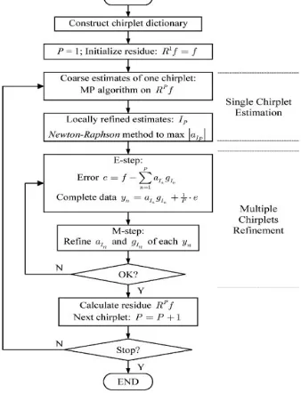
The algorithm was implemented using Matlab 7.0 on a system having configuration Pentium IV PC (3.0 GHz) & 1.0 GB memory. To estimate one chirplet from a 1200-point signal the average time taken was approximately 8 min. For each of the averaged signals, ten Gaussian chirplets were estimated with the algorithm described in Fig. 2.

Fig. 2- Adaptive decomposition algorithm flowchart.

Volume 3, Issue 3, March 2014

Page 406

, and a near zero chirp rate. The remaining two chirplets and had negative chirp rates, indicating that the instantaneous frequency decreased with time. Eventually, the local time-frequency structures that cannot be effectively matched by a single chirplet will be represented by several chirplets.

V. NOVEL FEATURE EXTRACTION ALGORITHM

Feature extraction algorithm for Brain-Computer Interfaces (BCIs) in which the new concept of fuzzy Region Of Interest (ROI) is used. This algorithm is based on inverse models. The relevant ROIs are automatically identified and their reactive frequency bands. It uses Support vector machine. It can automatically identify what are the relevant ROIs for mental task discrimination and in which frequency bands they react [11].

A. Parameters

 Statistical analysis: -

A statistical analysis comparing the different classes (mental tasks) was performed for each frequency and each voxel. The goal was to identify the voxels which activity for a given frequency can discriminate the classes.

 Clustering:-

A clustering algorithm is performed in order to gather voxels, which activity is statistically critical, into different ROIs.

 Fusion: -

ROIs found at similar spatial locations, in continuous frequencies, are fusionned and identified as reactive in the frequency band resulting from the concatenation of these frequencies.

 Adaptation:-

For each ROI obtained during fusion, another statistical analysis is performed in order to remove voxels that are not significant anymore in the reactive frequency band identified at the fusion step.

 Fuzzification: -

Each ROI is “fuzzified”, i.e., turned as a fuzzy ROI in order to properly define its spatial extension.

B. Methodology

 Statistical Analysis:

In this step statistical test is done for comparison. This test is individually done for each frequency. Analyzing all frequencies is obtained. It is called as substantial voxels as Members of the relevant ROIs.

 Clustering:

To perform aggregate of substantial voxels into different ROI’s clustering algorithm is used. For clustering a 4-dimensionnal vector is associated to each significant voxel. The coordinates are the 3D coordinates of the voxel in the chosen head model, and s is the voxel statistic computed at the previous step. When the clustering performed, all the voxels which corresponding vectors belong to the same cluster are aggregated into the same ROI. This step done, a set of relevant ROIs have been identified for each frequency.

 Fusion:

Relevant ROI’s are obtained for each frequency, now to decide which ROI’s are appropriate for which frequency band following procedure is followed:

Associate each ROI Ω found previously with the Frequency f at which it was found.

Among the whole set of couples (Ω; f), select two couples (Ω 1; f1) and (Ω 2; f2), such that the overlap

between Ω 1 and Ω 2 is high, and the frequency bands f1 and f2 are overlapped or are consecutive.

They consider an overlap is high if card (Ω 1 ∩ Ω 2) > 0:5 *min (card (Ω 1); card (Ω 2)) with card (Ω) being the number of voxels in.

Replace the couples (Ω 1; f1) and (Ω 2; f2) by the single couple (Ω 1U Ω 2; f1 Uf2). This means we

choose the union as the way of fusionning ROIs;

Return to point 2, until no more ROIs can be fusionned.

 Adaptation:

A ROI identified as reactive in the frequency band may contain voxels due to the use of the union as the fusion operator that were significant in a frequency between and but that are not substantial anymore in . The results found at this adaptation step are used for the next training step.

 Fuzzification and the concept of fuzzy ROI:

Any voxel carrying information should be in the ROI was derived, but that those with less information should be less in the ROI. A classical ROI is defined by the set of voxels it contains. The activity

Volume 3, Issue 3, March 2014

Page 407

Where is the activity of the voxel . A fuzzy ROI Ω f is not defined by a set of voxels anymore but by a fuzzy

membership function µ. This function provides the degree of membership, in [0; 1], of any existing voxel to the fuzzy ROI . This leads to fuzzy ROIs which boundaries are not well defined and therefore fuzzy. The activity of a fuzzy ROI is computed as follows:

With being the number of voxels in the whole head model. This formalism makes it possible to weigh each voxel according to its relative contribution in the ROI, and as such, use efficiently the whole of the available information. The shape of this function µ Ω depends on the inverse model and the statiscal test used [12].

C. Working Of The Algorithm

FuRIA is a generic algorithm as it is divided into different steps that can be used with different implementations for each of these steps. They chose to use sLORETA (standardized Low Resolution Electromagnetic TomogrAphy) as the inverse-model due to its good localization properties using sLORETA, computing the activity in a fuzzy ROI can be done using a simple matrix product:

Here, m is the vector of instantaneous measurements foreach one of the electrodes used, and a matrixsuch that . Therefore, computing theactivity in a fuzzy ROI is very fast [13].

VI. A SEMI SUPERVISED SUPPORT VECTOR MACHINES ALGORITHM.

A semi supervised SVM was applied for translating the features extracted from the electrical recordings of brain into control signals. This SVM classifier is built from a small labeled data set and a large unlabeled data set [17]. It is seen that in selective two different brain states common spatial pattern (CSP) is very. However, CSP needs a sufficient labeled data set. In order to overcome the drawback of CSP, it suggests a two-stage feature extraction method for the semi supervised learning algorithm. Apply algorithm to two BCI experimental data set [14].

B.Methods

 Dynamic CSP feature extraction:-

To classify the normal versus abnormal EEGs [16] and find spatial structures of event-related (de-)synchronization the common spatial patterns (CSP) is a method applied to EEG analysis. Two CSP features have been defined: (1) nonnormlized CSP feature (2) normalized CSP feature. The nonnormalized CSP feature is extracted directly from the covariance matrix of the raw or filtered EEG signal. The normalized CSP feature is extracted from the normalized covariance matrix of the raw or filtered EEG signal.

 Dynamic power feature extraction and the two-stage feature extraction method:-

The method is based on the following two facts: (1) the power feature extraction is not as dependent on sufficient labeled data set as CSP feature extraction; (2) the power feature is less powerful than CSP feature when the training data is sufficient.

 Semi supervised SVM:-

In this subsection, the semisupervised SVM introduced. Given a training set of labeled data

Where are the n dimensional features that have been labeled as ; and a set of unlabeled data

in , a semisupervised SVM was defined as:

Where is a penalty parameter, and are the slack variables that present the classification error of or .

Volume 3, Issue 3, March 2014

Page 408

 Batch-mode incremental training method:-

In this section the semisupervised SVM is extended. The division of the original unlabeled data set is done into several subsets, and marked them. Then mixed integer programming based on a subset. It is reasonable to assume that the users’ EEGs change gradually during the use of the BCI systems. The most confidently classified elements can be determined according to the distance between the element and the separating boundary. The criteria can be formulated as follows:

Where, constant is the distance threshold. The outline of the batch-mode incremental training method is as follows. Algorithm outline. Given two data sets: a labeled data set , and an unlabeled data set

Step 1: Equally divide the unlabeled data set Du into n subsets (for the online condition, these subsets canbe collected at several time intervals); then take Dl as the initial training set and let (i

denotes the loop of the algorithm); next extract dynamic power feature from data set and .

Step 2: Train an initial SVM classifier using the dynamic power features in .

Step 3:Estimate the labels of using the current classifier,then choose the most confidently classified elements using(7) and add them together with their predicted labels (we mark the most confidently classified elements with their predicted labels as set , to the training set that is, next we denote the remaining elements of as Qi.

Step 4. Run the mixed integer programming based on T and to get the labels of and adjust the parameters of the

SVM classifier; then add with predicted labels to that is,

Step 5. if i is smaller than or equals to M which denotes the number of steps for dynamic.power feature extraction, extract dynamic power features from ; otherwise, extract dynamic CSP features from Note that, for each loop, the transformation matrix of the dynamic CSP feature should be estimated again from the most confidently labeled elements of then use the new transformationmatrix to extract the dynamic CSP features from T again. Finally train a new SVM classifier based on the updated CSP features and their labels of

.

Step 6. If equals terminate; otherwise, go back to Step 3.

Additionally, since the size of the training set is enlarged during the training procedure, the penalty parameter C of the semisupervised SVM should adapt to this change. Thus, we extend the empirical formula for C introduced as:

Where denotes the loop. is the size of training set of the loop. is the size of unlabeled data set [15].

VII. COMPARATIVE ANALYSIS.

Volume 3, Issue 3, March 2014

Page 409

available [14]. By dividing the whole unlabeled data set into several subsets and employing selective learning, the batch mode incremental learning method significantly reduces the computational burden for training the semi supervised SVM.

VIII. CONCLUSION.

This paper presents study of EEG based algorithms in brain computer interface in which different algorithms like Wavelet Common Spatial Pattern (WCSP), which approaches distinguish between two classes of EEG data based & the Adaptive Chirplet Transform and Visual Evoked Potentials which deals with frequency space, chirplets exist as revolved. Also a Novel Feature Extraction Algorithm which contains five types of analysis & a Semi supervised Support Vector Machines Algorithm are analyzed.

References

[1] R.Wolpaw,N.Birbaumer,W.J.Heetdeks,D.J.Mcfarland,P.H.Peckham,G.Schalk,E.Donchin,La.Quatrano,C.J.Robinson And T.M.Vaughan,’Brain-Computer Interface Technology; A Review Of The First International Meeting,”Ieee Trans . Rehab. Eng.,Vol.8,Pp. 164-173,Jun 2000.

[2] G.S.Dean J. Krusienski,Dennis J.Mcfarland, Jonathan R. Woplaw,”A µ-Rhythm Matched Filter For Continuous Control Of Brain-Computer Interface,” IEEE Trans.Biomed.Eng.,Vol.54,No.2,Feburary 2007.

[3] Tanaka,K. Matsunaga, K. Wang H.O. Electroencephalogram- Based Control Of An Electric Wheelchair IEEE Trans Robotics,Vol.21,No.4,Auguest 2005.

[4] K. Ang, Z. Y. Chin, H. Zhang, and C. Guan, “Filter bank commonspatial pattern (FBCSP) in brain-computer interface,” in Proc. IEEE Int.Joint Conf. Neural Netw., Orlando, FL, USA, Jun. 2008, pp. 2390–2397.

[5] Y. B. Hua, Y. G. Zheng, Y. R. Guo, and W. Ting, “Adaptive subject based feature extraction in brain-computer interfaces using wavelet packet best basis decomposition,” Med. Eng. Phys., vol. 29, pp. 48–53, Mar. 2007.

[6] M. Vetterli and C. Herley, “Wavelets and filter banks: Theory and design,” IEEE Trans. Signal Process., vol. 40, no. 9, pp. 2207–2232, Sep. 1992.

[7] J. McFarland, L. M. McCane, S. V. David, and J. R.Wolfpaw, “Spatial filter selection for EEG-based communication,”

Electroencephalography Clin. Neurophysiol., vol. 103, pp. 386–394, Sep. 1997.

[8] S. Mann and S. Haykin, “The chirplet transform—physical considerations”, IEEE Trans. Signal Process., vol. 43, no. 11, pp. 2745–2761, Nov. 1995.

[9] Cohen, Time-Frequency Analysis. Upper Saddle River, N.J: Prentice Hall PTR, 1995.

[10]Davis, S. Mallat, and M. Avellaneda, “Adaptive greedy approxima tions ‘,Constructive Approximation, vol. 13, pp. 57–98, 1997.

[11]Congedo, F. Lotte, and A. L´ecuyer, .Classsification of move ment intention by spatially filtered electromagnetic inverse solutions,. Physics in Medicine and Biology, vol. 51, no. 8, pp. 1971.1989, 2006.

[12]A. Zadeh, .Fuzzy sets,. Fuzzy sets, fuzzy logic, and fuzzy systems: selected papers by Lotfi A. Zadeh, pp. 19.34, 1996.

[13]R. D. Pascual-Marqui, .Standardized low resolution brain electromag netic tomography (sloreta): technical details,.

Methods and Findings in Experimental and Clinical Pharmacology, vol. 24D, pp. 5.12, 2002.

[14]Seeger, “Learning with labeled and unlabeled data,” Tech. Rep., Institute for ANC, Edinburgh, UK, 2000.

[15]R. M. Karp, “Reducibility among combinatorial problems,” in Complexity of Computer Computations, R. E. Miller and J.W. Thatcher, Eds., pp. 85–103, Plenum Press,New York, NY, USA, 1972.

[16]http://en.wikipedia.org/wiki/Brain%E2%80%93computer_interface

[17]X. ZHU, “SEMI-SUPERVISED LEARNING WITH GRAPHS,” PH.D. DISSERTATION CARNEGIEMELLON UNIVERSITY, PITTSBURGH,PA,USA,2005.

[18]Zhang, T. B. Ho, M. S. Lin, and X. Liang, “Feature extraction for time series classification using discriminating wavelet coefficients,” in Proc. Int. Conf. Advances in Neural Netw., May 2006, vol. 3971, pp. 1394- 1399.

[19]——, Human Brain Electrophysiology: Evoked Potentials and Evoked Magnetic Fields in Science and Medicine. New York: Elsevier, 1989.

AUTHORS

Mr. Roshan M. Pote, ME (CSE) ,First Year,Department of CSE,Prof. Ram Meghe Institute Of Technology and Research, Badnera, Amravati. Sant Gadgebaba Amravati University, Amravati, Maharashtra, India – 444701.