Particle Swarm Optimization (PSO) Inspired Grey Wolf Optimization (GWO) Algorithm

(1)

Particle Swarm Optimization (PSO) Inspired

Grey Wolf Optimization (GWO) Algorithm

Yogendra Singh Kushwah#1, R.K. Shrivastava*2 #1

Research Scholar, Deptt. of Mathematics, S.M.S Govt. Science Collage, Jiwaji University, Gwalior, M.P. India

#2

Professor, Deptt. of Mathematics, S.M.S Govt. Science Collage, Jiwaji University, Gwalior, M.P. India

Abstract

This paper presents a new modified Grey Wolf Optimization (GWO) Algorithm inspired by the Particle Swarm Optimization (PSO) algorithm. The main features of the proposed algorithm called PSO Inspired Grey Wolf Optimization (PSOIGWO) is the integration of global best and inertia weights into the basic GWO algorithm that allows the better searching capability and quicker convergence. The combination of well-established features of PSO into the newly developed GWO algorithm provides an efficient hybrid algorithm which comprises the best features of the both algorithms. Experiments on standard optimization problems show the usefulness of the combined approach and its ability to efficiently and quickly search the solution.

Keywords - Global Optimization, Particle Swarm Optimization (PSO), Grey Wolf Optimization.

I. INTRODUCTION

The optimal solution is animportant requirement for many practical problems where the exact solution is either not feasible or difficult to find due to its complexity.The optimization approach is used in many branches of mathematics and engineering such structure designing, aerospace modeling, travelling postman problem etc. since the computation time requiredfor the exact solution finding methods, like branch andbound, dynamic programming, increases exponentially with the size of the instance to solve. The meta-heuristic algorithms are the best alternative of the best solution algorithms as it can provide an acceptable solution with in the required margin without computational complexity.

The meta-heuristic algorithms are not only simple but also have many interesting characteristics such as problem independency, adaptivenessand learning capabilities [2]. Most of the meta-heuristic algorithms uses natural (either physical or bio-intelligence) phenomena’s to find the solutions. Examples of the bio-intelligence inspired optimization algorithms are genetic algorithm, ant colony optimization, bee colony optimization, while the physical phenomenon inspired algorithms are water filling algorithm, particle swarm optimization, gravitational search algorithms etc. Although the meta-heuristic algorithms have several advantages but they also have some limitations as solution is not always guaranteed to be optimum the improper initialization could cause completely irrelative solution etc. hence for any meta-heuristic optimization algorithm these problems must be dealt properly. As sated above a number of meta-heuristic algorithms are already available but everyone has its own advantages and limitations which provide space for development of new algorithms one of such algorithm is Grey Wolf Optimization (GWO).

Grey wolf optimizer (GWO) algorithm described by Mirjalili [1] which is modeledfrom the hunting strategy of grey wolves. With results comparable to particle swarm optimization (PSO) and other optimization algorithms with fewer adjustable parameters and low complexity the GWO can be the preferable choice for deployment in practical applications. However like other optimization algorithms the GWO also has some limitations such as it can be easily trapped in the local optima when used with high-dimensional nonlinear objective functions. Furthermore the higher convergence speed of GWO makes it difficult to manage the balance between exploitation and exploration [3].

(2)

II. LITERATUREREVIEW

The GWO algorithm is firstly proposed by the Mirjalili [1] the algorithm applies the hunting strategy followed by the grey wolves, after that many modifications have been proposed to overcome the shortcomings of the algorithm some of them are discussed in this section. Wen Long et al. [3] proposed the use of a time-varying function of decreasing linearly for changing the value of vector 𝑎 which balances the exploration and exploitationabilities of the GWO. Furthermore the good-point-set method is employed for generating the initial population which enhances the global convergence of the algorithm. Aijun Zhu et al. [7] presented a hybrid GWO which utilizes the DE’s strong searching abilityto update the previous best positions of Alpha, Beta andDelta wolves, the position updating in such way makes GWO prone to the stagnation. Another modification of GWO is proposed by Narinder Singh et al. [8] which modifies the position update equation of standard GWO algorithm. The presented modification uses the mean of wolf position vectors for the estimation of movement direction of wolves. The use of exponential function for the decaying the value of vector 𝑎 is presented by Nitin Mittal et al. [9] the use of exponential decay function improves the exploitation and exploration capability of the algorithm.A Genetic Algorithm (GA) based initial population generation approach for GWO is presented by Qiang Li et al. [10], the proper initialization leads to greater possibility in finding global optimum. As with other meta-heuristic algorithms the GSO also requires proper initial value settings of variables to achieve the best results. Since these values depends upon problem under consideration and must be estimated on the basis of objective function characteristics to address this problem E. Emary et al [11] presented a reinforcement learning and neural network based approach EGWO (Experienced GWO) which evaluates the right parameters values for the algorithm. In their model the exploration rate of each wolf estimated bywolf’s own experienceand the current environment ofthe search space. The experience is storedin the form of neural network that maps agentstates to corresponding actions. The Powell local optimization based GWO algorithm PGWO is presented by Sen Zhang et al. [12]. This proposal uses Powell’s [16] conjugate direction method, is an algorithm used for finding a local minimum ofafunction. The Powell’s algorithm work with non-differentiable functions, and it takes no derivatives, this makes it suitable choice for deciding the direction of movement of wolf.

III.GREYWOLFOPTIMIZATION(GWO)

The Grey Wolf Optimization (GWO) was proposed by Mirjalili et al [4]. The GWO is inspired by the social structure and hunting behavior of grey wolves. The experimental results demonstrated its capabilities and excellent performance in solving many classical engineering design problems, such as spring tension, welded beam etc. [7].

The GWO technique considers the finding optimal solution problem as hunting of prey by grey wolves. The prey is equivalent to optimal solution. As the grey wolves hunting strategy involves three steps encircling prey, hunting, and attacking prey it also uses these approaches to find the optimal solution. The grey wolves strictly follows social hierarchy of leadership. In the hierarchy the group is led by the alpha (𝛼) wolf, which remains at the top of the hierarchy. After alpha the second level of wolves are called beta (𝛽) wolf similarly the third and fourth level wolves are called delta (𝛿) and omega (𝜔) respectively. The alpha wolf is followed by all (beta, delta and omega) wolves, while the beta wolves are followed by delta and omega, and delta wolves are followed by only omega. Since the omega remains in the lowest level they does not have any followers.

Now as the hunting is guided by alpha, beta and delta wolves and rest (omega) wolves just follow them. The movement of all the population in the optimization problem guided by the top three best solutions and these solutions are named as alpha, beta and delta respectively the rest of solutions are considered as omega.

A. Encircling the Prey

the first step of hunting is to encircle prey. The encircling process of grey wolves is equivalent to encircling the optimum solution by all population and it is given by:

𝐷 = 𝐶 ∙ 𝑋 𝑝𝑟𝑒𝑦 𝑖 − 𝑋 𝑤𝑜𝑙𝑓(𝑖) (1)

𝑋 𝑤𝑜𝑙𝑓 𝑖 + 1 = 𝑋 𝑝𝑟𝑒𝑦 𝑡 − 𝐴 ∙ 𝐷 (2)

Here 𝑖 represents the current iteration number, 𝐴 and 𝐶 are the coefficient vectors, 𝑋 𝑃𝑟𝑒𝑦 and 𝑋 𝑤𝑜𝑙𝑓 are the

position vectors of prey and wolf respectively. The coefficient vectors 𝐴 and 𝐶 are calculated as follows:

𝐴 = 2𝑎 ∙ 𝑟 1− 𝑎 (3)

(3)

Here the values of vector 𝑎 is linearly decreased from 2 to 0 with the iterations and 𝑟 1, 𝑟 2 are random vectors

bounded within the interval of [0, 1].

B. Hunting

In real hunting scenario the position of prey is known but in optimization problem the optimum solution is not known hence a rough estimation of optimum location is estimated by the alpha, beta and delta solutions knowing that they have the best knowledge of solution. The position update of wolves is done as follows:

𝑋 𝑤𝑜𝑙𝑓 𝑖 + 1 =𝑋 1+ 𝑋 ₃2+ 𝑋 3 ₍₅₎

where the𝑋 1, 𝑋 2 𝑎𝑛𝑑 𝑋 3 are estimated as:

𝑋 1= 𝑋 𝛼− 𝐴1∙ 𝐷𝛼 ,

𝐷𝛼 = 𝐶1∙ 𝑋𝛼− 𝑋𝑤𝑜𝑙𝑓 ,

(6)

𝑋 2= 𝑋 𝛽 − 𝐴2∙ 𝐷𝛽 ,

𝐷𝛽 = 𝐶1∙ 𝑋𝛽− 𝑋𝑤𝑜𝑙𝑓 ,

(7)

𝑋 3= 𝑋 𝛿− 𝐴3∙ 𝐷𝛿 ,

𝐷𝛿 = 𝐶1∙ 𝑋𝛿− 𝑋𝑤𝑜𝑙𝑓 ,

(8)

The equations 6, 7 and 8 assumes the location of prey (optimum solution) is the location of 𝛼, 𝛽 and 𝛿 respectively, then the mean location of prey is estimated by equation 5, and this is the location where the wolf (population) should move to get the prey (optimum).

C. Attacking

As the grey wolf start tightening their grip to prey the movement of prey becomes more and more smaller so as the movement of wolves, and at last the prey stops moving and wolf perform final attack. This scenario is simulated in mathematical model by decreasing the values of vector 𝑎 linearly from 2 to 0 with every iteration (as shown in equation 3), which limits the movements of prey (optimum location) and wolf (population locations) and finally it gets the prey (optimum).

Figure 1: the position updating process in GWO as presented by Mirjalili et al [4].

IV.PARTICLESWARMOPTIMIZATION(PSO)

(4)

𝑝𝑏𝑒𝑠𝑡

_𝑗

𝑝

𝑗𝑖+1

𝑔𝑏𝑒𝑠𝑡

𝑣

_𝑗𝑖

the search space. The particle positions are evolved to find the optimal solutions similarly as the bird ﬂocks searches for corn.

Figure 2: movement of particle in PSO [19].

The important properties of particles are they all knows the best solution found by particle itself up to current iteration as well as the best of all particles solutions found till current iteration, these positions are known as 𝑝𝑏𝑒𝑠𝑡 (particle’s best) and 𝑔𝑏𝑒𝑠𝑡 (global best). The positions of particles are evolved using these two values till the solution found, the complete process can be described in following steps:

D. Initialization

firstly the particles are randomly positioned all over the search space. For example let there be 𝑛 number of total particles whose location can be defined as {𝑝1, 𝑝2, 𝑝3, … . 𝑝𝑛}.

E. Finding the fitness

each of the generated particles are evaluated for the provided objective function, let for the 𝑗𝑡𝑕 particle

𝑝𝑗 the locations and fitness values till 𝑖𝑡𝑕 generation be

𝑃𝑗𝑖 = 𝑝𝑗1, 𝑝𝑗2, 𝑝𝑗3, … . . , 𝑝𝑗𝑖−1, 𝑝𝑗𝑖 , and 𝐹𝑗𝑖= {𝑓𝑗1, 𝑓𝑗2, 𝑓𝑗3, … . . , 𝑓𝑗𝑖−1, 𝑓𝑗𝑖} respectively. So the particle 𝑝𝑗 will

remember it location related to the best value of 𝐹𝑗𝑖 which can be defined as 𝑝𝑏𝑒𝑠𝑡𝑗. Similarly it will also

remember the values of best location related to the best values of {𝑝𝑏𝑒𝑠𝑡1, 𝑝𝑏𝑒𝑠𝑡2, 𝑝𝑏𝑒𝑠𝑡3, … … , 𝑝𝑏𝑒𝑠𝑡𝑛} which

is named as 𝑔𝑏𝑒𝑠𝑡.

Location Update: now each particle updates their location using their 𝑝𝑏𝑒𝑠𝑡 and 𝑔𝑏𝑒𝑠𝑡 as follows:

𝑝𝑗𝑖+1= 𝑝𝑗𝑖+ 𝑣𝑗𝑖+1 (9)

𝑣𝑗𝑖+1= 𝜔𝑣𝑗𝑖+ 𝑐1𝑟1 𝑝𝑏𝑒𝑠𝑡𝑗− 𝑝𝑗𝑖 + 𝑐2𝑟2(𝑔𝑏𝑒𝑠𝑡

− 𝑝𝑗𝑖) (10)

𝜔 = 𝜔𝑚𝑎𝑥 − 𝜔𝑚𝑖𝑛 𝑖𝑡𝑒𝑟_{𝑖𝑡𝑒𝑟}𝑚𝑎𝑥 − 𝑖

𝑚𝑎𝑥 (11)

Where the 𝑟1 and𝑟2 are the random variable within the range [0, 1], and 𝑐1 and 𝑐2 are the trust coefficient

which defines the weightage 𝑝𝑏𝑒𝑠𝑡 and 𝑔𝑏𝑒𝑠𝑡 in the of movement ofparticle. The 𝜔 represents the inertia of the particle this controls the exploration capabilities of the algorithm.

These three parameters are problem dependent and can be fine-tuned depending upon the nature of the problem.

F. Termination

(5)

V. PARTICLESWARMOPTIMIZATIONINSPIREDGREYWOLFOPTIMIZATION(PSOIGWO)

Looking into the both GWO and PSO algorithms it can be seen that GWO uses 𝛼, 𝛽 and 𝛿 wolf positions to find the solution location (equation 5) and then it updates positions of all the wolves, while the PSO uses 𝑔𝑏𝑒𝑠𝑡, 𝑝𝑏𝑒𝑠𝑡 and inertia (𝜔) (equation 10).

The involvement of inertia in PSO increases the exploration capability, while the knowledge of 𝑔𝑏𝑒𝑠𝑡 and 𝑝𝑏𝑒𝑠𝑡 keeps track on best locations of the particles encountered which increases its capabilities of both exploitation and exploration.

The proposed algorithm uses equivalents of these parameters to improve the performance of GWO as follows: The position of the wolves in GWO modified using

𝑋 𝑤𝑜𝑙𝑓 𝑡 + 1 =

𝑋 1+ 𝑋 2+ 𝑋 3

3 (12)

In proposed algorithm this is considered as the equivalent to 𝑔𝑏𝑒𝑠𝑡 as they actually represents the mean of best three.

Next the 𝑝𝑏𝑒𝑠𝑡 and inertia (𝜔) are estimated in same way as in the standard PSO algorithm.So the position estimation equation for the PSO inspired GWO is defined as follows:

𝑋 𝑗𝑖+1= 𝑓𝑑∙ 𝜔𝑋 𝑗𝑖+ 𝑐1∙ 𝑓𝑑∙ 𝑟1 𝑝𝑏𝑒𝑠𝑡 + 𝑐𝑗 2(1

− 𝑓𝑑∙ 𝑟2)(𝑔𝑏𝑒𝑠𝑡 )

(13)

Since 𝑐1 and 𝑐2 are set to 1, the above equation can be re written as:

𝑋 𝑗𝑖+1= 𝑓𝑑∙ 𝜔𝑋 𝑗𝑖+ 𝑓𝑑∙ 𝑟1 𝑝𝑏𝑒𝑠𝑡 + (1 − 𝑓𝑗 𝑑

∙ 𝑟2)(𝑔𝑏𝑒𝑠𝑡 )

(14)

Where the 𝑓𝑑 (decay factor) and 𝑔𝑏𝑒𝑠𝑡 are given by

𝑓𝑑 =

𝑎 2

2

(15)

𝑔𝑏𝑒𝑠𝑡 =𝑋 1+ 𝑋 2+ 𝑋 3

3 (16)

where𝑟1 and 𝑟2 are the random variables in the range [-1, 1] unlike the PSO where it remains in the range [0,

1]. The 𝑎 is GWO linearly decreasing variable from 2 to 0.

The application of 𝑓𝑑 decays the impact of inertia, 𝑝𝑏𝑒𝑠𝑡 and randomness in 𝑔𝑏𝑒𝑠𝑡 these all terms are

adopted PSO features. Hence it can be said that the algorithm initially uses the PSO features for exploration of search space and then gradually shifts to GWO for convergence.

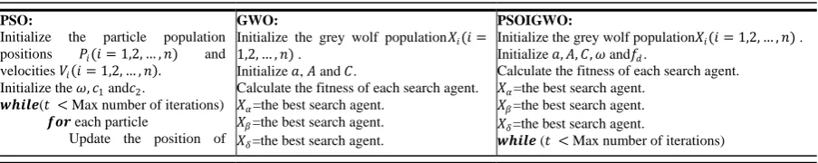
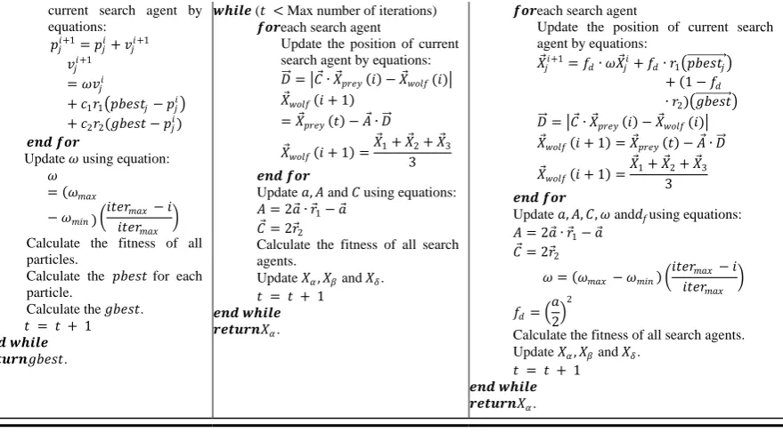
The comparison of the algorithm in pseudo code is provided in table 1.

Table 1: pseudo codes for PSO, GWO and PSOIGWO.

PSO:

Initialize the particle population positions 𝑃𝑖(𝑖 = 1,2, … , 𝑛) and velocities 𝑉𝑖 𝑖 = 1,2, … , 𝑛 .

Initialize the 𝜔, 𝑐1 and𝑐2.

𝒘𝒉𝒊𝒍𝒆(𝑡 < Max number of iterations)

𝒇𝒐𝒓 each particle

Update the position of GWO:

Initialize the grey wolf population𝑋𝑖(𝑖 =

1,2, … , 𝑛) . Initialize 𝑎, 𝐴 and 𝐶.

Calculate the fitness of each search agent.

𝑋𝛼=the best search agent.

𝑋𝛽=the best search agent.

𝑋𝛿=the best search agent.

PSOIGWO:

Initialize the grey wolf population𝑋𝑖(𝑖 = 1,2, … , 𝑛) . Initialize 𝑎, 𝐴, 𝐶, 𝜔 and𝑓𝑑.

Calculate the fitness of each search agent.

𝑋𝛼=the best search agent.

𝑋𝛽=the best search agent.

𝑋𝛿=the best search agent.

(6)

current search agent by equations:

𝑝_𝑗𝑖+1_{= 𝑝} 𝑗𝑖+ 𝑣𝑗𝑖+1

𝑣𝑗𝑖+1

= 𝜔𝑣𝑗𝑖

+ 𝑐1𝑟1 𝑝𝑏𝑒𝑠𝑡𝑗− 𝑝𝑗𝑖

+ 𝑐2𝑟2(𝑔𝑏𝑒𝑠𝑡 − 𝑝𝑗𝑖)

𝒆𝒏𝒅 𝒇𝒐𝒓

Update 𝜔 using equation:

𝜔

= 𝜔𝑚𝑎𝑥

− 𝜔𝑚𝑖𝑛

𝑖𝑡𝑒𝑟𝑚𝑎𝑥− 𝑖

𝑖𝑡𝑒𝑟𝑚𝑎𝑥 Calculate the fitness of all particles.

Calculate the 𝑝𝑏𝑒𝑠𝑡 for each particle.

Calculate the 𝑔𝑏𝑒𝑠𝑡.

𝑡 = 𝑡 + 1 𝒆𝒏𝒅 𝒘𝒉𝒊𝒍𝒆

𝒓𝒆𝒕𝒖𝒓𝒏𝑔𝑏𝑒𝑠𝑡.

𝒘𝒉𝒊𝒍𝒆 (𝑡 < Max number of iterations)

𝒇𝒐𝒓each search agent

Update the position of current search agent by equations:

𝐷 = 𝐶 ∙ 𝑋 𝑝𝑟𝑒𝑦 𝑖 − 𝑋 𝑤𝑜𝑙𝑓(𝑖)

𝑋 𝑤𝑜𝑙𝑓 𝑖 + 1

= 𝑋 𝑝𝑟𝑒𝑦 𝑡 − 𝐴 ∙ 𝐷

𝑋 𝑤𝑜𝑙𝑓 𝑖 + 1 =

𝑋 1+ 𝑋 2+ 𝑋 3

3 𝒆𝒏𝒅 𝒇𝒐𝒓

Update 𝑎, 𝐴 and 𝐶 using equations:

𝐴 = 2𝑎 ∙ 𝑟 1− 𝑎

𝐶 = 2𝑟 2

Calculate the fitness of all search agents.

Update 𝑋𝛼, 𝑋𝛽 and 𝑋𝛿.

𝒓𝒆𝒕𝒖𝒓𝒏𝑋𝛼.

𝒇𝒐𝒓each search agent

Update the position of current search agent by equations:

𝑋 𝑗𝑖+1= 𝑓𝑑∙ 𝜔𝑋 𝑗𝑖+ 𝑓𝑑∙ 𝑟1 𝑝𝑏𝑒𝑠𝑡 𝑗

+ 1 − 𝑓𝑑

∙ 𝑟2 𝑔𝑏𝑒𝑠𝑡

𝐷 = 𝐶 ∙ 𝑋 𝑝𝑟𝑒𝑦 𝑖 − 𝑋 𝑤𝑜𝑙𝑓(𝑖)

𝑋 𝑤𝑜𝑙𝑓 𝑖 + 1 = 𝑋 𝑝𝑟𝑒𝑦 𝑡 − 𝐴 ∙ 𝐷

𝑋 𝑤𝑜𝑙𝑓 𝑖 + 1 =

𝑋 1+ 𝑋 2+ 𝑋 3

3 𝒆𝒏𝒅 𝒇𝒐𝒓

Update 𝑎, 𝐴, 𝐶, 𝜔 and𝑑𝑓using equations:

𝐴 = 2𝑎 ∙ 𝑟 1− 𝑎

𝐶 = 2𝑟 2

𝜔 = 𝜔𝑚𝑎𝑥− 𝜔𝑚𝑖𝑛

𝑖𝑡𝑒𝑟𝑚𝑎𝑥− 𝑖

𝑖𝑡𝑒𝑟𝑚𝑎𝑥

𝑓𝑑=

𝑎 2

2

Calculate the fitness of all search agents. Update 𝑋𝛼, 𝑋𝛽 and 𝑋𝛿.

𝒓𝒆𝒕𝒖𝒓𝒏𝑋𝛼.

VI.SIMULATIONRESULTS

To evaluate the capabilities of the proposed PSOIGWO algorithm, is tested against 23 classical and popular benchmark test problems listed in [7, 19]. The test functions can be divided into three different group’s unimodal functions, multimodal functions and ﬁxed-dimensionmultimodal functions. The details of the functions and their plots are provided in table 2-4 and figure 3-5 respectively. To evaluate the performance of the proposed algorithm four parameters named best, worst, average and standard deviation are used. These performance parameters are obtained for each benchmark test function by repeatedly evaluating them for 50 times. To evaluate the comparative performance of the proposed algorithm these results are compared with the GWO, PSO, GA and DE algorithms. For the comparison following configurations are used each algorithm.

Table 2: Algorithm configurations used for comparison.

Algorithm Parameter’s Name Parameter’s Value

PSOIGWO

𝑐1 1

𝑐2 1

𝜔𝑚𝑎𝑥 0.8

𝜔𝑚𝑖𝑛 0.2

𝑃𝑎𝑝𝑢𝑙𝑎𝑡𝑖𝑜𝑛 𝑆𝑖𝑧𝑒 25

𝑀𝑎𝑥𝑖𝑚𝑢𝑚 𝐼𝑡𝑒𝑟𝑎𝑡𝑖𝑜𝑛𝑠 500

GWO 𝑃𝑎𝑝𝑢𝑙𝑎𝑡𝑖𝑜𝑛 𝑆𝑖𝑧𝑒 25

HGWO

𝑠𝑐𝑎𝑙𝑖𝑛𝑔 𝑓𝑎𝑐𝑡𝑜𝑟 𝐹 0.5

𝐶𝑟𝑜𝑠𝑠𝑜𝑣𝑒𝑟 𝑃𝑟𝑜𝑏 𝑃𝑐 0.2

𝑃𝑎𝑝𝑢𝑙𝑎𝑡𝑖𝑜𝑛 𝑆𝑖𝑧𝑒 25

PSO

𝑐1 2

𝑐2 2

𝜔𝑚𝑎𝑥 0.9

𝜔𝑚𝑖𝑛 0.1

(7)

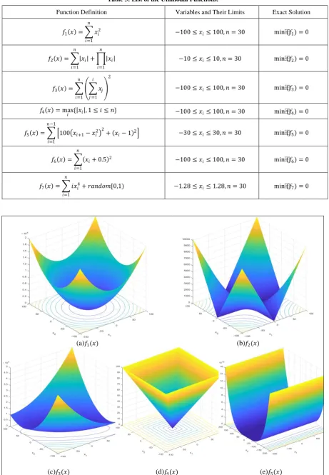
Table 3: List of the Unimodal Functions.

Function Definition Variables and Their Limits Exact Solution

𝑓1 𝑥 = 𝑥𝑖2 𝑛

𝑖=1

−100 ≤ 𝑥𝑖≤ 100, 𝑛 = 30 min⁡(𝑓1) = 0

𝑓2 𝑥 = 𝑥𝑖 𝑛

𝑖=1

+ 𝑥𝑖

𝑛

𝑖=1

−10 ≤ 𝑥𝑖≤ 10, 𝑛 = 30 min⁡(𝑓2) = 0

𝑓3 𝑥 = 𝑥𝑗 𝑖

𝑗 =1 2 𝑛

𝑖=1

−100 ≤ 𝑥𝑖≤ 100, 𝑛 = 30 min⁡(𝑓3) = 0

𝑓4 𝑥 = max_𝑖 { 𝑥𝑖 , 1 ≤ 𝑖 ≤ 𝑛} −100 ≤ 𝑥_𝑖≤ 100, 𝑛 = 30 min⁡(𝑓₄) = 0

𝑓5 𝑥 = 100 𝑥𝑖+1− 𝑥𝑖2 2

+ 𝑥𝑖− 1 2 𝑛−1

𝑖=1

−30 ≤ 𝑥𝑖≤ 30, 𝑛 = 30 min⁡(𝑓5) = 0

𝑓6 𝑥 = 𝑥𝑖+ 0.5 2 𝑛

𝑖=1

−100 ≤ 𝑥𝑖≤ 100, 𝑛 = 30 min⁡(𝑓6) = 0

𝑓7 𝑥 = 𝑖𝑥𝑖4+ 𝑟𝑎𝑛𝑑𝑜𝑚[0,1) 𝑛

𝑖=1

−1.28 ≤ 𝑥𝑖≤ 1.28, 𝑛 = 30 min⁡(𝑓7) = 0

(a)𝑓1(𝑥) (b)𝑓2(𝑥)

(8)

(f)𝑓6(𝑥) (g)𝑓7(𝑥) Figure 3: showing the plots of unimodal functions presented in table 2.

Table 4: List of the Multimodal Functions.

𝑓8 𝑥 = −𝑥𝑖sin⁡( 𝑥𝑖 ) 𝑛

𝑖=1

−500 ≤ 𝑥𝑖≤ 500, 𝑛 = 30 min 𝑓8 = −4189.829_{× 𝑛}

𝑓9 𝑥 = 𝑥𝑖2− 10 cos 2𝜋𝑥𝑖 + 10 𝑛

𝑖=1

, −5.12 ≤ 𝑥𝑖≤ 5.12, 𝑛 = 30 min⁡(𝑓9) = 0

𝑓10 𝑥 = −20 exp −0.2

1 𝑛 𝑥𝑖2

𝑛

𝑖=1

− exp 1

𝑛 𝑐𝑜𝑠 2𝜋𝑥𝑖

𝑛

𝑖=1

+ 20 + 𝑒,

−32 ≤ 𝑥𝑖≤ 32, 𝑛 = 30 min⁡(𝑓10) = 0

𝑓11 𝑥 =

1 4000 𝑥𝑖2

𝑛

𝑖=1

− cos 𝑥𝑖 𝑖 + 1,

𝑛

𝑖=1

−600 ≤ 𝑥𝑖≤ 600, 𝑛 = 30 min⁡(𝑓11) = 0

𝑓12 𝑥 =𝜋_𝑛{10 sin 𝜋𝑦𝑖

+ 𝑦𝑖− 1 2[1 𝑛−1

𝑖=1

+ 10 sin2_𝜋𝑦 𝑖+1

+ 𝑦𝑛− 1 2]}

+ 𝑢 𝑥𝑖, 10,100,4 𝑛

𝑖=1

𝑦𝑖= 1 +𝑥𝑖₄+ 1,

𝑢 𝑥𝑖, 𝑎, 𝑘, 𝑚 =

𝑘 𝑥𝑖− 𝑎 𝑚, 𝑥𝑖> 𝑎

0, −𝑎 ≤ 𝑥𝑖≤ 𝑥

𝑘 −𝑥𝑖− 𝑎 𝑚, 𝑥𝑖< −𝑎

−50 ≤ 𝑥𝑖≤ 50, 𝑛 = 30

min⁡(𝑓12) = 0

𝑓13 𝑥 = 0.1 sin2 3𝜋𝑥𝑖

+ 𝑥𝑖− 1 2[1 𝑛

𝑖=1

+ sin2_(3𝜋𝑥

𝑖)] + 𝑥𝑖+ 1 2[1

+ sin2_(2𝜋𝑥 𝑛)]

+ 𝑢(𝑥𝑖, 5,100,4) 𝑛

𝑖=1

,

(9)

(a)𝑓8(𝑥) (b)𝑓9(𝑥) (c)𝑓10(𝑥)

(d)𝑓11(𝑥) (e)𝑓12(𝑥) (f)𝑓13(𝑥)

Figure 4: showing the plots of multimodal functions presented in table 3.

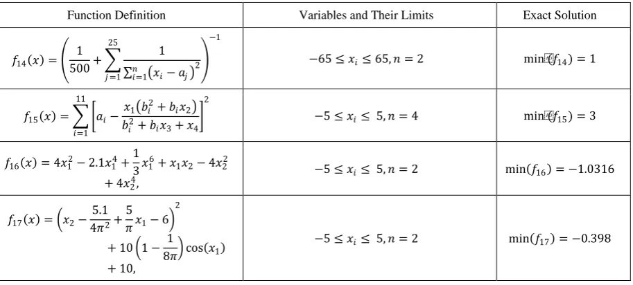
Table 5: List of the Fixed Dimension Multimodal Functions.

𝑓14 𝑥 = ₅₀₀1 + 1

𝑥𝑖− 𝑎𝑗 2 𝑛

𝑖=1 25

𝑗 =1

−1

−65 ≤ 𝑥𝑖≤ 65, 𝑛 = 2 min⁡(𝑓14) = 1

𝑓15 𝑥 = 𝑎𝑖−𝑥1 𝑏𝑖 2_{+ 𝑏}

𝑖𝑥2

𝑏_𝑖2_{+ 𝑏} 𝑖𝑥3+ 𝑥4

2 11

𝑖=1

−5 ≤ 𝑥𝑖≤ 5, 𝑛 = 4 min⁡(𝑓15) = 3

𝑓16 𝑥 = 4𝑥12− 2.1𝑥14+

1

3𝑥16+ 𝑥1𝑥2− 4𝑥22

+ 4𝑥24,

−5 ≤ 𝑥𝑖≤ 5, 𝑛 = 2 min 𝑓16 = −1.0316

𝑓17 𝑥 = 𝑥2−_4𝜋5.12+

5 𝜋𝑥1− 6

2

+ 10 1 − 1

8𝜋 cos 𝑥1 + 10,

(10)

𝑓18 𝑥 = 1 + 𝑥1+ 𝑥2+ 1 2 19 − 14𝑥1

+ 3𝑥12− 14𝑥2+ 6𝑥1𝑥2

+ 3𝑥22 30

+ 2𝑥1− 3𝑥2 2 18

− 32𝑥1+ 12𝑥12+ 48𝑥2

− 36𝑥1𝑥2+ 27𝑥22 ,

−2 ≤ 𝑥𝑖≤ 2, 𝑛 = 2 min 𝑓18 = 3

𝑓19 𝑥 = 𝑐𝑖exp − 𝑎𝑖𝑗 𝑥𝑗− 𝑝𝑖𝑗 2 𝑛

𝑗 =1 4

𝑖=1

1 ≤ 𝑥𝑖≤ 3, 𝑛 = 3 min 𝑓19 = 3.86

𝑓20 𝑥 = 𝑐𝑖exp − 𝑎𝑖𝑗 𝑥𝑗 − 𝑝𝑖𝑗 2 𝑛

𝑗 =1 4

𝑖=1

0 ≤ 𝑥𝑖≤ 1, 𝑛 = 6 min 𝑓20 = −3.32

𝑓21 𝑥 = − 𝑥 − 𝑎𝑖 𝑥 − 𝑎𝑖 𝑇+ 𝑐𝑖 −1 5

𝑖=1

0 ≤ 𝑥𝑖≤ 10, 𝑛 = 4 min 𝑓21 = −10.1532

𝑓22 𝑥 = − 𝑥 − 𝑎𝑖 𝑥 − 𝑎𝑖 𝑇+ 𝑐𝑖 −1 7

𝑖=1

0 ≤ 𝑥𝑖≤ 10, 𝑛 = 4 min 𝑓22 = −10.4028

𝑓23 𝑥 = − 𝑥 − 𝑎𝑖 𝑥 − 𝑎𝑖 𝑇+ 𝑐𝑖 −1 10

𝑖=1

0 ≤ 𝑥𝑖≤ 10, 𝑛 = 4 min 𝑓23 = −10.5363

(a)𝑓14(𝑥) (b)𝑓15(𝑥) (c)𝑓16(𝑥)

(11)

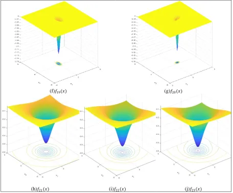
(f)𝑓19(𝑥) (g)𝑓20(𝑥)

(h)𝑓21(𝑥) (i)𝑓22(𝑥) (j)𝑓23(𝑥)

Figure 5: showing the plots of multimodal functions presented in table 4.

Table 6: Evaluation and Comparison of Best Results. Unimodal Functions

function Exact Solution PSOIGWO GWO PSO GA DE

𝑓1(𝑥) 0 5.73312E-81 1.19156E-27 1.15737E-03 1.08515E-01 6.41676E-02

𝑓2(𝑥) 0 2.29022E-43 3.86384E-16 1.89361E+00 2.17493E+00 2.28411E-03

𝑓3(𝑥) 0 1.63830E-54 1.38199E-07 6.82600E+04 4.87321E+00 2.44008E+02

𝑓4(𝑥) 0 3.37323E-35 1.13011E-07 1.21886E+02 1.24059E+00 1.64606E+01

𝑓5(𝑥) 0 2.58802E+01 2.59425E+01 1.31698E+03 2.10619E+00 2.73052E+02

𝑓6(𝑥) 0 5.22899E-01 1.50290E-04 1.18912E-03 2.41504E-01 4.58609E-01

𝑓7(𝑥) 0 8.72565E-05 4.40180E-04 5.10906E+00 7.02064E-01 8.97338E-02 Multimodal Functions.

PSOIGWO GWO PSO GA DE

𝑓8(𝑥) -12569.487 -1.02004E+04 -7.43762E+03 -5.75454E+2 -5.58382E+02 -1.04188E+04

𝑓9(𝑥) 0 0.00000E+00 5.68434E-14 8.47039E+01 1.01643E+01 3.04228E+01

𝑓10(𝑥) 0 4.44089E-15 1.18128E-13 2.09643E+01 1.53522E+00 1.86102E+00

𝑓11(𝑥) 0 0.00000E+00 0.00000E+00 1.74743E-03 7.17464E-03 3.98328E-02

𝑓12(𝑥) 0 2.45736E-02 1.33638E-02 3.22578E+00 1.05966E-02 4.17999E-01

𝑓13(𝑥) 0 5.57171E-01 2.47707E-01 3.87094E+00 1.27219E-02 2.96557E+00 Fixed Dimension Multimodal Functions.

𝑓14(𝑥) 1 9.98004E-01 9.98004E-01 9.98004E-01 1.07632E+01 9.98004E-01

𝑓15(𝑥) 0.00030 3.07611E-04 3.07601E-04 1.19064E-03 7.28637E-04 3.07486E-04

(12)

𝑓17(𝑥) 0.398 3.97887E-01 3.97887E-01 3.97887E-01 3.97887E-01 3.97887E-01

𝑓18(𝑥) 3 3.00000E+00 3.00000E+00 3.00000E+00 3.00000E+00 3.00000E+00

𝑓19(𝑥) -3.86 -3.86278E+00 -3.86278E+00 0.00000E+00 -3.86278E+00 -3.86278E+00

𝑓20(𝑥) -3.32 -3.32199E+00 -3.32199E+00 0.00000E+00 -3.32200E+00 -3.32200E+00

𝑓21(𝑥) -10.1532 -1.01530E+01 -1.01530E+01 -1.01532E+01 -1.01532E+01 -1.01532E+01

𝑓22(𝑥) -10.4028 -1.04028E+01 -1.04027E+01 -1.04029E+01 -1.04029E+01 -1.04029E+01

𝑓23(𝑥) -10.5363 -1.05360E+01 -1.05360E+01 -1.05364E+01 -1.05364E+01 -1.05364E+01

Table 6: Evaluation and Comparison of Worst Results. Unimodal Functions

𝑓1(𝑥) 0 5.97424E-74 1.82667E-24 7.71682E+00 3.63538E+00 1.81294E+03

𝑓2(𝑥) 0 2.94281E-38 7.64921E-15 7.75558E+40 1.00655E+01 6.19411E+00

𝑓3(𝑥) 0 2.70203E-44 1.33103E-02 6.65502E+06 1.47210E+02 2.34668E+03

𝑓4(𝑥) 0 4.41039E-30 1.12640E-05 8.04105E+02 2.95263E+00 5.71032E+01

𝑓5(𝑥) 0 2.88005E+01 2.87683E+01 6.54249E+07 4.06518E+02 1.64963E+06

𝑓6(𝑥) 0 2.53379E+00 1.76372E+00 1.61236E+02 1.76519E+01 7.47995E+02

𝑓7(𝑥) 0 3.74774E-03 6.38262E-03 3.30940E+05 1.66857E+01 4.70505E-01 Multimodal Functions.

𝑓8(𝑥) -12569.487 -3.89086E+03 -3.07866E+03 -1.10083E+02 -4.12515E+02 -5.47418E+03

𝑓9(𝑥) 0 0.00000E+00 2.44096E+01 9.97946E+02 6.32870E+01 1.92381E+02

𝑓10(𝑥) 0 7.99361E-15 3.70370E-13 2.13342E+01 3.06378E+00 1.33922E+01

𝑓11(𝑥) 0 0.00000E+00 3.10384E-02 7.67146E-01 2.73973E-01 9.99982E+00

𝑓12(𝑥) 0 2.01877E-01 5.76287E-01 7.12867E+08 7.06768E-01 7.45479E+05

𝑓13(𝑥) 0 2.41035E+00 1.47133E+00 1.41027E+05 6.88525E-01 2.87328E+06 Fixed Dimension Multimodal Functions.

𝑓14(𝑥) 1 1.07632E+01 1.26705E+01 1.55038E+01 1.45631E+01 1.07632E+01

𝑓15(𝑥) 0.00030 2.03634E-02 2.03634E-02 2.18017E-03 2.30309E-02 2.03633E-02

𝑓16(𝑥) -1.0316 -1.03163E+00 -1.03163E+00 -2.15464E-01 -2.15464E-01 -1.03163E+00

𝑓17(𝑥) 0.398 3.97957E-01 3.97914E-01 3.97887E-01 3.97887E-01 3.97887E-01

𝑓18(𝑥) 3 3.00080E+00 8.40001E+01 8.40000E+01 8.40000E+01 3.00000E+00

𝑓19(𝑥) -3.86 -3.85681E+00 -3.85489E+00 0.00000E+00 -1.00082E+00 -3.86278E+00

𝑓20(𝑥) -3.32 -3.13847E+00 -3.02235E+00 0.00000E+00 -3.20074E+00 -3.18514E+00

𝑓21(𝑥) -10.1532 -3.41617E+00 -2.63013E+00 -2.63047E+00 -2.63047E+00 -2.63047E+00

𝑓22(𝑥) -10.4028 -5.08760E+00 -5.08762E+00 -1.83759E+00 -1.83759E+00 -2.76590E+00

𝑓23(𝑥) -10.5363 -3.83531E+00 -2.42160E+00 -1.67655E+00 -1.67655E+00 -2.42734E+00

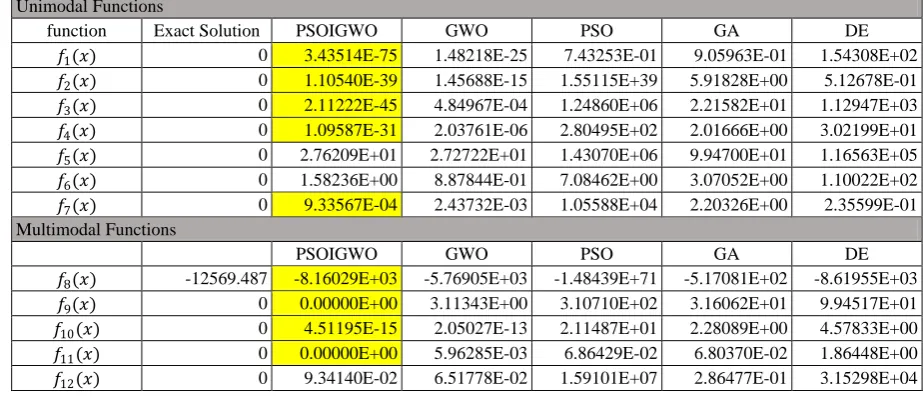
Table 8: Evaluation and Comparison of Average Results. Unimodal Functions

function Exact Solution PSOIGWO GWO PSO GA DE

𝑓1(𝑥) 0 3.43514E-75 1.48218E-25 7.43253E-01 9.05963E-01 1.54308E+02

𝑓2(𝑥) 0 1.10540E-39 1.45688E-15 1.55115E+39 5.91828E+00 5.12678E-01

𝑓3(𝑥) 0 2.11222E-45 4.84967E-04 1.24860E+06 2.21582E+01 1.12947E+03

𝑓4(𝑥) 0 1.09587E-31 2.03761E-06 2.80495E+02 2.01666E+00 3.02199E+01

𝑓5(𝑥) 0 2.76209E+01 2.72722E+01 1.43070E+06 9.94700E+01 1.16563E+05

𝑓6(𝑥) 0 1.58236E+00 8.87844E-01 7.08462E+00 3.07052E+00 1.10022E+02

𝑓7(𝑥) 0 9.33567E-04 2.43732E-03 1.05588E+04 2.20326E+00 2.35599E-01 Multimodal Functions

𝑓8(𝑥) -12569.487 -8.16029E+03 -5.76905E+03 -1.48439E+71 -5.17081E+02 -8.61955E+03

𝑓9(𝑥) 0 0.00000E+00 3.11343E+00 3.10710E+02 3.16062E+01 9.94517E+01

𝑓10(𝑥) 0 4.51195E-15 2.05027E-13 2.11487E+01 2.28089E+00 4.57833E+00

𝑓11(𝑥) 0 0.00000E+00 5.96285E-03 6.86429E-02 6.80370E-02 1.86448E+00

(13)

𝑓13(𝑥) 0 1.18332E+00 8.22504E-01 3.64029E+03 1.78862E-01 3.06647E+05 Fixed Dimension Multimodal Functions

𝑓14(𝑥) 1 2.33542E+00 5.51611E+00 2.98717E+00 1.21745E+01 1.39101E+00

𝑓15(𝑥) 0.00030 3.66615E-03 4.06751E-03 1.79814E-03 2.56545E-03 1.87705E-03

𝑓16(𝑥) -1.0316 -1.03163E+00 -1.03163E+00 -9.01042E-01 -1.01531E+00 -1.03163E+00

𝑓17(𝑥) 0.398 3.97894E-01 3.97890E-01 3.97887E-01 3.97887E-01 3.97887E-01

𝑓18(𝑥) 3 3.00009E+00 4.62007E+00 1.70400E+01 8.40000E+00 3.00000E+00

𝑓19(𝑥) -3.86 -3.86211E+00 -3.86106E+00 0.00000E+00 -3.64008E+00 -3.86278E+00

𝑓20(𝑥) -3.32 -3.25338E+00 -3.27757E+00 0.00000E+00 -3.25764E+00 -3.24786E+00

𝑓21(𝑥) -10.1532 -7.92965E+00 -9.51189E+00 -5.32892E+00 -5.54997E+00 -8.13711E+00

𝑓22(𝑥) -10.4028 -9.23216E+00 -1.00818E+01 -5.48814E+00 -4.96282E+00 -8.66517E+00

𝑓23(𝑥) -10.5363 -9.31027E+00 -1.03718E+01 -4.14082E+00 -4.19933E+00 -9.66556E+00

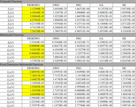
Table 9: Evaluation and Comparison of Standard DeviationResults. Unimodal Functions

𝑓1(𝑥) 1.13396E-74 2.69266E-25 1.66374E+00 8.13535E-01 2.95330E+02

𝑓2(𝑥) 4.36546E-39 1.32875E-15 1.09680E+40 2.04803E+00 1.02999E+00

𝑓3(𝑥) 5.96944E-45 1.92228E-03 1.86078E+06 2.87813E+01 5.42933E+02

𝑓4(𝑥) 6.27561E-31 1.80660E-06 1.03376E+02 5.03672E-01 8.22575E+00

𝑓5(𝑥) 8.21158E-01 7.93564E-01 9.23711E+06 8.13696E+01 2.67122E+05

𝑓6(𝑥) 4.74129E-01 4.26683E-01 3.17071E+01 3.20128E+00 1.78668E+02

𝑓7(𝑥) 7.54238E-04 1.38837E-03 4.98531E+04 2.49356E+00 8.34265E-02

Multimodal Functions

𝑓8(𝑥) 1.51016E+03 9.35468E+02 8.14214E+71 4.23001E+01 1.12532E+03

𝑓9(𝑥) 0.00000E+00 6.06477E+00 1.96301E+02 9.65077E+00 3.90375E+01

𝑓10(𝑥) 5.02430E-16 6.45630E-14 9.33279E-02 3.32551E-01 2.18245E+00

𝑓11(𝑥) 0.00000E+00 9.33413E-03 1.32577E-01 5.48832E-02 2.25803E+00

𝑓12(𝑥) 4.02251E-02 7.88044E-02 1.01249E+08 1.71622E-01 1.09763E+05

𝑓13(𝑥) 3.37832E-01 2.52039E-01 1.99611E+04 1.61148E-01 6.02454E+05 Fixed Dimension Multimodal Functions

𝑓14(𝑥) 2.66955E+00 4.55991E+00 2.94990E+00 8.86815E-01 1.59533E+00

𝑓15(𝑥) 7.36411E-03 7.71527E-03 1.19158E-04 4.07410E-03 4.11825E-03

𝑓16(𝑥) 3.44073E-08 3.47382E-08 3.02249E-01 1.15423E-01 2.37376E-16

𝑓17(𝑥) 1.34584E-05 5.19163E-06 4.06345E-09 3.15912E-09 3.36448E-16

𝑓18(𝑥) 1.55692E-04 1.14551E+01 2.99966E+01 1.44321E+01 2.87453E-15

𝑓19(𝑥) 1.30359E-03 2.71072E-03 0.00000E+00 6.07517E-01 3.14018E-15

𝑓20(𝑥) 6.84498E-02 8.09129E-02 0.00000E+00 6.00007E-02 5.86834E-02

𝑓21(𝑥) 2.59848E+00 1.97063E+00 2.80483E+00 2.36077E+00 2.78313E+00

𝑓22(𝑥) 2.22344E+00 1.27457E+00 3.13909E+00 2.45880E+00 2.98448E+00

(14)

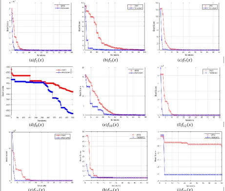
(a)𝑓1(𝑥) (b)𝑓3(𝑥) (c)𝑓7(𝑥)

(d)𝑓8(𝑥) (e)𝑓10(𝑥) (f)𝑓12(𝑥)

(g)𝑓13(𝑥) (h)𝑓18(𝑥) (i)𝑓23(𝑥)

Figure 6: Convergence curve for different functions.

From Table VI it can be seen that the PSOIGWO, compared to standard GWO, PSO,GA and DE algorithms, provide best values for five Unimodal functions𝑓1 𝑥 , 𝑓2 𝑥 , 𝑓3 𝑥 , 𝑓4 𝑥 , 𝑓7 𝑥 , one Multimodal

function 𝑓10(𝑥) it outperforms all other algorithms by large margin, while for Fixed Dimension MultimodalFunctions it provides the same best results obtained by other algorithm. Even for the remaining functions in Unimodal and Multimodal group it remains competitive.

Comparing for worst results from Table VII the PSOIGWOprovide best values for six Unimodal functions 𝑓1 𝑥 , 𝑓2 𝑥 , 𝑓3 𝑥 , 𝑓4 𝑥 , 𝑓5(𝑥), 𝑓7 𝑥 , four Multimodal function 𝑓9 𝑥 , 𝑓10 𝑥 , 𝑓11 𝑥 , 𝑓12(𝑥) it

outperforms all other algorithms by large margin, while for Fixed Dimension MultimodalFunctions it provides the same best results obtained by other algorithm. For the remaining functions in all groups it remains competitive.

Comparing for average results from Table VIII the PSOIGWOprovide best values for five Unimodal functions 𝑓1 𝑥 , 𝑓2 𝑥 , 𝑓3 𝑥 , 𝑓4 𝑥 , 𝑓7 𝑥 , four Multimodal function 𝑓8 𝑥 , 𝑓9 𝑥 , 𝑓10 𝑥 , 𝑓11 𝑥 and six

FixedDimension MultimodalFunctions𝑓16 𝑥 , 𝑓17 𝑥 , 𝑓18 𝑥 , 𝑓19 𝑥 , 𝑓22 𝑥 , 𝑓23 𝑥 , it outperforms all other algorithms by large margin, while for remainingfunctions either it provides the same best results obtained by other algorithm or at least remains competitive.

Comparing for standard deviation results from Table IX the PSOIGWOprovide the lowest deviation for five Unimodal functions𝑓1 𝑥 , 𝑓2 𝑥 , 𝑓3 𝑥 , 𝑓4 𝑥 , 𝑓7 𝑥 , four Multimodal function 𝑓8 𝑥 , 𝑓9 𝑥 , 𝑓10 𝑥 , 𝑓11 𝑥 it

(15)

VII. CONCLUSION

The proposed PSOIGWO algorithm utilizes the exploration capabilities of PSO and convergence capability GWO to achieve the best of both. The comparative analysis of the algorithm for the 23 standard test benchmark function shows that for most of Unimodal functions and Multimodal functions it outperforms the other algorithms with large margin, while for Fixed Dimension Multimodalfunctions it provides the same best results obtained by other algorithm. The analysis also shows that for most cases the PSOIGWO remains first or second best. The algorithm also shows best stability as for five Unimodal functions, four Multimodal functions and six Fixed Dimension Multimodalfunctions it gives the lowest deviation. The algorithm also shows quick convergence than the standard GWO algorithm as shown in figure 6.

REFERENCES

[1] SeyedaliMirjalili, Seyed Mohammad Mirjalili, Andrew Lewis “Grey Wolf Optimizer”, Advances in Engineering Software 69 (2014) 46–61.

[2] VoratasKachitvichyanukul “Comparison of Three Evolutionary Algorithms: GA, PSO, and DE”, Industrial Engineering & Management Systems Vol. 11, No 3, September 2012, pp.215-223.

[3] Wen Long, SongjinXu “A Novel Grey Wolf Optimizer for Global Optimization Problems”, Advanced Information Management, Communicates, Electronic and Automation Control Conference (IMCEC), 2016 IEEE.

[4] E. Emary, WaleedYamany, Aboul Ella Hassanien and Vaclav Snasel “Multi-Objective Grey-Wolf Optimization for Attribute Reduction”, International Conference on Communication, Management and Information Technology (ICCMIT2015).

[5] Ali Parsian, Mehdi Ramezani, NoradinGhadimi “A hybrid neural network-grey wolf optimization algorithm for melanoma detection”, Biomedical Research 2017; 28 (8): 3408-3411.

[6] M.R. Mosavi, M. Khishe, A. Ghamgosar “Classification of Sonar Data Set Using Neural Network Trained By Grey Wolf Optimization”, Neural Network World 4/2016, 393–415.

[7] Aijun Zhu, ChuanpeiXu, Zhi Li, Jun Wu, and Zhenbing Liu “Hybridizing grey wolf optimization with differential evolution for global optimization and test scheduling for 3D stacked SoC” Journal of Systems Engineering and Electronics Vol. 26, No. 2, April 2015, pp.317–328.

[8] Narinder Singh and SB Singh “A Modified Mean Grey Wolf Optimization Approach for Benchmark and Biomedical Problems”, Evolutionary Bioinformatics Volume 13: 1–28 © the Author(s) 2017.

[9] Nitin Mittal, Urvinder Singh, and Balwinder Singh Sohi “Modified Grey Wolf Optimizer for Global Engineering Optimization”, Hindawi Publishing Corporation Applied Computational Intelligence and Soft Computing Volume 2016, Article ID 7950348, 16 pages. [10] iang Li, Huiling Chen, Hui Huang, Xuehua Zhao, ZhenNaoCai, Changfei Tong, Wenbin Liu, and XinTian “An Enhanced Grey Wolf

Optimization Based Feature Selection Wrapped Kernel Extreme Learning Machine for Medical Diagnosis”, Hindawi Computational and Mathematical Methods in Medicine Volume 2017, Article ID 9512741, 15 pages.

[11] E.Emary, Hossam M. Zawbaa, and CrinaGrosan “Experienced Grey Wolf Optimization through Reinforcement Learning and Neural Networks”, IEEE Transactions on Neural Networks and Learning Systems 2017.

[12] Sen Zhang and Yongquan Zhou “Grey Wolf Optimizer Based on Powell Local Optimization Method for Clustering Analysis”, Hindawi Publishing Corporation Discrete Dynamics in Nature and Society Volume 2015, Article ID 481360, 17 pages.

[13] E.Emary, Hossam M. Zawbaa “Impact of Chaos Functions on Modern Swarm Optimizers”, PLoS ONE 11(7): e0158738. doi:10.1371/journal.pone.0158738 2016.

[14] QifangLuo, Sen Zhang, Zhiming Li and Yongquan Zhou “A Novel Complex-Valued Encoding Grey Wolf Optimization Algorithm”, Algorithms, Volume 9, 2016.

[15] Riccardo Poli, James Kennedy, Tim Blackwell “Particle swarm optimization, an overview”, Swarm Intelligence June 2007, Volume 1, Issue 1, pp 33–57.

[16] Gerhard Venter, JaroslawSobieszczanski-Sobieski “Particle Swarm Optimization”, AIAA Journal, Vol. 41, No. 8 (2003), pp. 1583-1589.

[17] James Kennedy and Russell Eberhart “Particle Swarm Optimization”, Proceedings of the 1995 IEEE International Conference on Neural Network.

[18] B.Y. Qu, J.J. Liang, Z.Y. Wang, Q. Chen, P.N. Suganthan “Novel benchmark functions for continuous multimodal optimization with comparative results”, Swarm and Evolutionary Computation 26 (2016) 23–34.