A Non-linear Integer Bi-level Programming Model for Competitive Facility Location of Distribution Centers

Please cite this article as: B. Yousefi Yegane, I. Nakhai Kamalabadi, H. Farughi, A Non-linear Integer Bi-level Programming Model for Competitive Facility Location of Distribution Centers, International Journal of Engineering (IJE), TRANSACTIONSB: Applications Vol. 29, No. 8, (August 2016) 1131-1140

International Journal of Engineering

A Non-linear Integer Bi-level Programming Model for Competitive Facility Location

of Distribution Centers

B. Yousefi Yegane*, I. Nakhai Kamalabadi, H. Farughi

Department of Industrial Engineering, University of Kurdistan, Kurdistan, Iran

P A P E R I N F O

Paper history:

Received 23 May 2016

Received in revised form 24 June 2016 Accepted 14 July 2016

Keywords: Bi-level Programming Competitive Facility Location Ant Colony Algorithm Supply Chain

A B S T R A C T

The facility location problem is a strategic decision-making for a supply chain which determines the profitability and sustainability of its components. This paper deals with a scenario where two supply chains, consisting of a producer, a number of distribution centers and several retailers provided with similar products, compete to maintain their market shares by opening new distribution centers because of increasing demand. The competition problem is formulated as a non-linear integer bi-level mathematical model, where the upper level represents the decisions of the leader producer and the lower level administrates the decisions of the follower producer. It has been shown that even in small-scale problems, level mathematical programming problems are strongly NP-hard, so an adapted bi-level ant colony algorithm with inter-bi-level information sharing is developed to solve the problem.To evaluate the performance of the developed ant colony algorithm, the upper bound of the competitive facility location problem is determined by solving the upper-level problem as an integer linear programming model without considering the follower’s decision. Comparing the computational results of the developed ant colony algorithm with those of the determined upper bounds shows the satisfactory capability of the proposed approach for solving even medium- and large-scale problems.

doi: 10.5829/idosi.ije.2016.29.08b.13

1. INTRODUCTION1

The facility location problem is a branch of operation research with great significance from both practical and combinatorial optimization perspectives. Facility location is an effective tool which easily facilitates its goal by reducing transportation costs and accelerating the rate of return of investment [1]. The classical location problem is concerned with determination of the location of a project to optimize the allocation of facilities to customers. Competitive facility location is a special case of the location problem where at least two decision-makers, simultaneously or consequently, start to seek maximum market shares to optimize their objective functions by opening new distribution centers, but not before giving due consideration to the strength of the competitors. The special case where only two competitors attempt to open their distribution centers is

1_{*Corresponding Author’s Email: [email protected] (B.}

Yousefi Yegane)

location with regard to the number of facilities, their locations and their types (product variety and capacity of the facility); they formulated the problem as a nonlinear integer programming model and obtained its solutions through two heuristic algorithms, the greedy algorithm and the steepest descent algorithm. Beresnev [9] followed a new approach by formulating the CFL problem as a bi-level programming model, and then presented a new method for determining the upper bound of the problem; in this model, both competitors were seeking to maximize their profits.

Saidani et al. [10] studied the facility location problem by considering the responses of competitors in the market and used Huff’s attractiveness function to determine the market share. Ashtiani et al. [11] used robust programming to determine the optimum solution of the competitive facility location problem with the aim of maximizing market share for competitors, under assumption of an unknown number of follower centers. Beresnev [12] continued his research on the competitive facility location problem by developing a branch and bound method to determine an optimum solution. Rahmani and MirHassani [13] studied the competitive facility location problem as a bi-level mathematical programming model; using Lagrangian relaxation method they obtained acceptable solutions for their mathematical model; their results indicated that the proposed method was highly efficient. MirHassani et al. [14] used a modified particle swarm optimization algorithm to solve the competitive location problem and compared their results with the upper bound obtained from solving a mathematical model; based on the conducted analysis, their results showed the capability of the proposed meta-heuristic algorithm of obtaining high-quality solutions. Although the competitive location problem has been the subject of much research, analyzing the problem as a bi-level mathematical programming model is a somewhat neglected approach (Beresnev [12]), and few studies on this subject include the studies of Beresnev ([9, 12, 15, 16]), Rahmani and MirHassani [13] and MirHassani et al. [14].

Increase in consumption of foodstuff such as dairy products and prepared or semi-prepared food and even introduction of a new product by one or several producers can affect the market balance. Thus, when the level of production or the capacity of existing distribution centers cannot meet the market’s demand, each producer, depending on its strength, attempts to survive in the competitive market by increasing the value of production or opening new distribution centers; on the other hand, in markets of products such as food and medicine, each customer may satisfy his own demand with more than one producer or distributer center, and each producer seeks to gain the maximum market share in order to keep its customers and increase their satisfaction level, supplying the demands of one or all of its customers through more than one distribution

center; as these assumptions are not considered in studies similar to this research, our developed mathematical model can be used by numerous industries such as dairy manufacturers, pharmaceutical producers and cosmetic and healthcare industries.

The main objective of the current study is to develop a mathematical model for the competitive facility location problem with the highest degree of adaptability to real-world applications; for example, each producer can spend a limited budget on expanding the distribution centers or production sites, which has not been considered by many researchers up to now. As a results of budget limitation, the producer can open only a few distribution centers among the set of candidate locations. In distribution of commodities such as dairy products, supplying a customer with only one distribution center may not be economically justified, so in this paper, we assume that each distribution center can cover more than one customer and each customer can satisfy his demand with more than one distribution center.

In view of the above points, the bi-level competitive facility location problem presented by Beresnev [12] will be studied and developed as a bi-level mathematical programming model through applying the following changes:

1. Facility location will be subject to budget constraint; 2. The two competitors have an initial market share and try to keep it by creating new centers;

3. New distribution centers only cover customers that are being covered by the current distribution centers of each producer (the new distribution centers of the leader are only used to supply the customers that are covered by the existing distribution centers of the leader, and vice versa);

4. Each customer can satisfy his demand from more than one distribution center of each producer (only the leader or the follower);

5. Each distribution center can cover more than one customer;

6. The profit gained from covering different customers with distribution centers may be different.

Further information about competitive facility location can be found in the works of Kress and Pesch [17] and Drezner [18].

2. BI-LEVEL MATHEMATICAL PROGRAMMING MODEL FOR COMPETITIVE FACILITY LOCATION PROBLEM

the two competitors start to open new distribution centers to deal with growth of market demand.

Suppose that the two competitors operate with a non-cooperative behavior based on game theory approach; the main feature of the non-cooperative games is that each player looks for his own benefit. The Nash and Stackelberg equilibriums are the most important methods used in many non-cooperative games. The Nash equilibrium is used when the players of a game choose their strategies simultaneously; but in a leader-follower scenario, the leader can act before the follower; in this case, the optimal strategy of each player can be determined through the Stackelberg equilibrium.

The Nash equilibrium applies when the players do not cooperate with each other and determine their decisions simultaneously (like in playing rock-paper-scissors). A Stackelberg game is used in a non-cooperative and sequential decision making process. In this game, one player acts as a leader and another plays as a follower. The leader first chooses his decision taking the follower’s reaction into account, and then the follower sees this decision and selects his best decision [19]. The Stackelberg equilibrium consists of two concepts: the leader and the follower. This equilibrium is applicable when one of the players can move before the other players and play as the leader.

In other words, the leader has more power than the follower, and hence in this game, the leader makes the first decisions. Afterwards, the follower makes his own decisions according to the decisions of the leader. In a leader-follower environment, the follower chooses the best response to the decision of the leader, and the leader optimizes his objective function according to the follower’s response.

Accordingly, the competitive location problem will be formulated as a non-linear integer bi-level programming model with regard to the following assumptions (It should be noted that bi-level programming is a representation of Stackelberg game). 1. Two supply chains each of them with one producer, multiple distribution centers and several retailers are considered;

2. The decision-making of the competitors is based on the Stackelberg game;

3. Each distribution center can cover more than one customer;

4. Each customer is covered only by leader or follower distribution centers;

5. The demand of each customer can be satisfied through more than one distribution center;

6. Distribution must be done through distribution centers, and direct shipping from producers to retailers is not allowed;

7. Each producer supplies only a part of the market.

First, the parameters of the problem are introduced, and following that, the bi-level formulation of the competitive facility location problem is presented.

Indices

Indices for leader

Indices for follower

Indices for customer

Indices for distribution centers

Parameters

Number of potential locations;

Number of existent DCs of leader;

Number of existent DCs of follower;

Number of customers;

The maximum number of customers that each DC can

serve;

Setup cost of DC of leader;

Setup cost of DC of follower;

Total budget of leader to open new DCs;

Total budget of follower to open new DCs;

Net profit of delivered products from new DC i

tocustomer j;

̃ products from existentNet profit of delivered leaders’ DC i to customer j;

̌ products from existentNet profit of delivered followers’ DC i to customer j;

Decision variable

{

{

̂ ̂ _{

{

{

̂

̂

According to the definitions of the parameters, a non-linear integer bi-level programming model of the competitive facility location problem is presented as follows:

[∑ (∑ ∑ ( )

∑ (∑ ̃ ̂ ( ̂ )))] ∑ (1)

∑ (2)

(3)

∑ ̂ (4)

∑ ̂ (5)

̂ (6)

* + (7)

* + (8)

̂ * + (9)

[∑ {∑ ∑ ̌ ̂ }] *∑ + (10) (11)

∑ (12)

(13)

̂ ̂ (14)

̂ (15)

∑ ̂ (16)

∑ ̂ (17)

* + (18)

* + (19)

̂ * + (20)

Equation (1) determines the objective function of the leader with respect to lost profit due to customer served by the new and existing distribution centers of the follower; the leader’s budget constraint to open new centers is presented by Equation (2); constraint (3) ensures product distribution through opened distribution

centers; constraints (4) indicates that the demand of each customer can be supplied by all of the distribution centers of the leader; constraint (5) indicates the maximum number of customers served by each of the existing distribution centers of the leader, Equation (6) states that new distribution centers deliver products only to customers who are covered by existing centers; Equations (7) to (9) represent the status of upper-level decision variables; Equation (10) states the objective function of the follower producer, which aims to maximize profit through opening new distribution centers and also through using existing distribution centers; Equation (11) ensures that at every candidate location, only the leader or follower can open a new distribution center; constraint (12) represents the budget constraint of the follower; constraint (13) acts like constraint (3) but at the upper level; customer segmentation for the two competitors based on existing distribution centers is stated by Equation (14), meaning that for each customer, the product will be delivered only by one of the two competitors; constraint (15) acts like constraint (6) but at the upper level; constraints (16) and (17) act like constraints (4) and (5); constraints (18)-(20) define lower-level decision variables just like constraints (6) -(8).

In this model, the upper-level decision-maker determines his strategy, and then the lower-level decision-maker, knowing this strategy, determines his policy to optimize his own objective function, and lastly, the optimum response of the leader is determined based on the best response of the follower.

Jeroslow [20] proved that even in small scale, a bi-level mathematical programming problem is strongly NP-hard; thus, several heuristic and meta-heuristic methods have been developed to deal with the high complexity of bi-level mathematical programming problems.

Beresnev [12] used a branch-and-bound algorithm to solve the bi-level competitive facility location problem and introduced a technique to determine an upper bound for the problem. MirHassani et al. [14] used a modified version of particle swarm optimization algorithm to solve the competitive facility location problem as a bi-level mathematical programming model. Farvaresh and Sepehri [21] presented a branch-and-cut method by defining valid inequalities based on Steiner tree for the bi-level mathematical programming problem. Several researchers have used meta-heuristic techniques to solve bi-level mathematical programming; more information about numerous metaheuristic methods proposed to solve bi-level mathematical problems can be found in the work of El-Ghazali [22].

bi-level mathematical programming problems can be classified into four categories:

I. Nested Sequential Approach In this category,

the lower-level problem must be solved by an exact, heuristic or metaheuristic method based on the results generated for the upper-level problem, and the result of the lower-level problem must be used to re-solve the upper-level problem, and this process must be repeated until the stopping criteria are met.The main flaw of this approach is the complexity of the process, since for each solution obtained at each stage for the upper-level problem, the optimal solution of the lower-level problem must also be determined.

II. Single-level Transformation Approach In

this approach, first, a technique such as Karush–Kuhn– Tucker conditions must be used to transform the bi-level mathematical programming problem to a single-level model, and it must then be solved by an exact, heuristic or metaheuristic method.

III. Multi-objective Approach In this category,

the bi-level problem must be transformed into a single-level multi-objective model; linking between the pareto-optimal solution of a multi-objective problem and solution space of a bi-level problem is the most important part of the method. This technique has been used in only a few studies (El-Ghazali [22]).

IV. Co-evolutionary Approach In this approach,

each level of the problem must be solved by a separate meta-heuristic algorithm; the information of the two levels must then be shared, and the process of parallel solution must continue until a termination criterion is achieved.The most important point in this approach is how to share information between two levels of the problem.This approach also requires a particular segment of memory to be dedicated to shared information. Figure 1 shows the general framework of this method.

In this study, the bi-level mathematical model is solved by a co-evolutionary approach in which both levels are solved by ant colony algorithm simultaneously.

Metaheuristic 1 Metaheuristic 2

Upper level population of solutions

lower level population of solutions

Evaluation of solution (x,y) Generate (x,y)

Evaluation of solution (x,y) Generate (x,y) Information

exchange

Figure 1. General framework of co-evolutionary solution to

bi-level problem [22]

To evaluate the performance of the proposed algorithm, the upper bound of the problem is developed based on the approach described in Section 4, and the results of ant colony algorithm are compared with this bound.

3. THE PROPOSED ANT COLONY ALGORITHM

In this study, each level of the bi-level mathematical problem is solved by the ant colony algorithm proposed by Dorigo and Gambardella [23]. The discussed problem is a three-level supply chain consisting of a producer for each supply chain, a number of distribution centers and several retailers, which can all be represented on a network.The arcs between the first and second levels represent the products flowing from producers to distribution centers, and those between the second and third levels represent delivery of the products from distribution centers to retailers. It should be noted that in this network, direct shipment from producers to retailers is not allowed.The general structure of the used ant colony algorithm is described in the following:

Algorithm (1)

Step 0. Set all problem parameters (including the number of ants of the two competitors, the initial pheromone path, etc.)

Until termination condition holds do:

Step 1. Given the number of leader (follower) ants, repeat the following steps:

Step 1. 1. Use the selection rule to generate an initial solution;

Step 1. 2. If this solution is not acceptable2, go to step 1-3; otherwise, use algorithm (2) to convert it into an acceptable solution;

Step 1. 3. Add the resulting acceptable solution to the Tabu list3;

Step 2. If the solution of the previous step pertains to the leader, repeat step 1 for the follower; otherwise, go to step 3;

Step 3. Alter the pheromone path with both local and global updating rules;

Step 4. If the termination condition does not hold, go to step 1; otherwise, go to step 5;

Step 5. Select the best solution;

Step 6. End.

2_{-Acceptable solution is a solution whose cost does not exceed the} total available budget.

1. 3. Selection Rule Artificial ants use a probability law inspired by the behavior of natural ants for consecutive selection of distribution centers for both competitors and construction of a solution with respect to data obtained via a pheromone path which is updated over time. Based on the system designed by Dorigo and Gambardella [23], each ant of the leader or the follower uses the following rule to select the new distribution center with probability of ( ), where signifies the follower and signifies the leader.

{ } (21)

where denotes the pheromone path, represents the heuristic information of distribution center and is a value between 0 and 1, signifying the importance of ; in a particular iteration of the algorithm, distribution center is selected with a probability of (

) according to the following probability distribution:

∑ (22)

Parameter is determined based on the two rules of nearest and most profitable distribution center, as shown below.

Parameter is calculated for each potential location:

∑ (23)

In addition, based on the rule of nearest location, parameter is calculated as follows:

∑ (24)

and finally:

{ } (25)

After generating solutions based on algorithm (1), the costs of some of the generated solutions may exceed the total available budget, so algorithms (2) is used to convert these solutions into acceptable solutions.

Algorithm (2)

Step 1. Select among the not-selected centers the one with the highest benefit-cost ratio for the leader (follower), and insert it in place of selected center with the highest cost.

Step 2. As long as cost is higher than budget, repeat step 1.

The following rule is used for local updating of pheromone in each iteration:

( ) (26)

where is considered for each competitor. The following relationship is used for global updating of the pheromone path based on the best found solution,which, at this stage, is the most profitable distribution center:

( ) ( ⁄ ) (27)

After the termination of both algorithms 1 and 2, a new ant colony algorithm is run to maximize the profits of product delivery.

Algorithm (3)

Step 0. Set all parameters for all new and existing distribution centers of the two competitors (number of ants, initial pheromone value, and probability of acceptance);

Step 1. Repeat the following steps for all new and existing leader (follower) centers and all ants in these centers;

Step 1. 1. Use the selection rule to generate an initial solution for the existing distribution centers (specifying the customers to which each distribution center is allowed to send the product);

Step 1. 2. Use the selection rule to generate a solution for new distribution centers only for customers selected in the previous step;

Step 1. 3. Add the resulting solution (selected customers) to the ban list;

Step 2. If the solution of the previous step pertains to the leader, repeat step 1 for the follower; otherwise, go to step 3;

Step 3. Alter the pheromone path with both local and global updating rules;

Step 4. If the termination condition does not hold, go to step 1; otherwise, go to step 5;

Step 5. Select the best solution (the objective function, new distribution centers and covered customers);

Step 6. End.

Local and global pheromone path updating rules are similar to those used for selection of new distribution centers but do not necessarily employ the parameters of the previous step.

It should be mentioned that the profits gained from delivery through new and existing distribution centers are expressed as a matrix, where is the number of existing or new distribution centers of the two competitors, and is the number of customers. Each distribution center covers only a certain number of customers, which is based on its profit threshold; in this study, this threshold is defined as { } for all

existing and new distribution centers of the two competitors.

4. DETERMINING AN UPPER BOUND FOR THE COMPETITIVE LOCATION PROBLEM

Theorem.The upper bound for the objective function of the competitive location problem can be determined by solving the following problem:

[∑ (∑ ∑ ̃ ̂ )]

∑ (28)

∑ (29)

(30)

∑ ̂ (31)

∑ ̂ (32)

̂ (33)

* + (34)

* + (35)

̂ * + (36)

Proof. Please see appendix A.

5. COMPUTATIONAL RESULTS

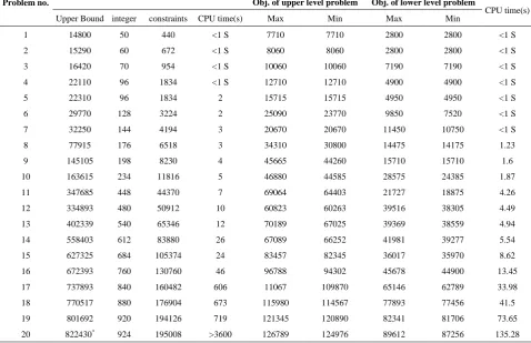
To evaluate the performance of the developed ant colony algorithm, 20 test problems were generated, and then, the upper bound of each problem was determined by the mathematical programming model presented in Section 4.

These values were then compared with the results of the developed ant colony algorithm. Table1 shows the obtained upper bound for the objective function of the leader-follower problem and the objective function values of the upper-level and lower-level problems calculated by ant colony algorithm.

The proposed ant colony algorithm was coded in VB 6.0, and was run ten times for each test problem on a computer with Core i5 processor and 4GB RAM under 64-bit Windows 7 operating system.The upper bound of each instance problem was determined with Lingo 9.0 software.

In all instances, the profit of the existing and new distribution centers and the cost of setting up a new distribution center were generated randomly from the intervals [500,2500], [1000,3500], and [2000,4000] in that order.

TABLE 1. Computational results for test problems

Ant colony results Upper level problem

Problem no.

CPU time(s) Obj. of lower level problem

Obj. of upper level problem

6. CONCLUSION

This paper deals with a location problem with two supply chains consisting of one producer, a number of distribution centers and several retailers, where each producer obtains a portion of the market share by delivering its products through distribution centers. The leader producer establishes new distribution centers to exploit the new market demand due to increase in market demand, and the follower reacts by opening its own new distribution centers. These two competitors choose new distribution centers among several potential locations based on the rules of Stackelberg game and their own strength. The problem was described as a bi-level mathematical model, and then, because of its high complexity, an adopted ant colony algorithm was developed to achieve high-quality solutions. Compared to similar researches, the bi-level mathematical model of this paper is more compatible with the real world because new distribution centers are opened based on budget constraint, such as what happens in real world, each distribution center in the model can serve more than one customer or retailer whilst each retailer could be supplied by more than one distributor.To evaluate the capability of the proposed ant colony algorithm, an upper bound was developed for the problem, and the results were compared with the upper bound; the comparison showed the high performance of the proposed approach to obtain high-quality and near-optimal solutions. Our suggestions for future research on this problem include examination of other problems such as relocating of one or more than one distribution center, development of better upper bounds with different approaches, use of different methods of product distribution such as vehicle routing and hybrid delivery approaches as well as other methods of transport that could make the problem more conforming with real-world applications.

1. Shishebori, D., "Study of facility location-network design problem in presence of facility disruptions: A case study (research note)", International Journal of Engineering-Transactions A: Basics, Vol. 28, No. 1, (2014), 97-108. 2. Hotelling, H., ''Stability in competition'', The Economic

Journal, Vol. 39, (1929), 41-57

3. Teitz, M. B., "Locational strategies for competitive systems†", Journal of Regional Science, Vol. 8, No. 2, (1968), 135-148. 4. Huff, D. L., "Defining and estimating a trading area", The

Journal of Marketing, (1964), 34-38.

5. Hakimi, S. L., "On locating new facilities in a competitive environment", European Journal of Operational Research,

Vol. 12, No. 1, (1983), 29-35.

6. Labbe, M. and Hakimi, S. L., "Market and locational equilibrium for two competitors", Operations Research, Vol. 39, No. 5, (1991), 749-756.

7. Pal, D. and Sarkar, J., "Spatial competition among multi-store firms", International Journal of Industrial Organization, Vol. 20, No. 2, (2002), 163-190.

8. Aboolian, R., Berman, O. and Krass, D., "Competitive facility location model with concave demand", European Journal of Operational Research, Vol. 181, No. 2, (2007), 598-619. 9. Beresnev, V., "Upper bounds for objective functions of discrete

competitive facility location problems", Journal of Applied and Industrial Mathematics, Vol. 3, No. 4, (2009), 419-432. 10. Saidani, N., Chu, F. and Chen, H., "Competitive facility location

and design with reactions of competitors already in the market", European Journal of Operational Research, Vol. 219, No. 1, (2012), 9-17.

11. Ashtiani, M. G., Makui, A. and Ramezanian, R., "A robust model for a leader–follower competitive facility location problem in a discrete space", Applied Mathematical Modelling, Vol. 37, No. 1, (2013), 62-71.

12. Beresnev, V., "Branch-and-bound algorithm for a competitive facility location problem", Computers & Operations Research, Vol. 40, No. 8, (2013), 2062-2070.

13. Rahmani, A. and MirHassani, S., "Lagrangean relaxation-based algorithm for bi-level problems", Optimization Methods and Software, Vol. 30, No. 1, (2015), 1-14.

14. MirHassani, S., Raeisi, S. and Rahmani, A., "Quantum binary particle swarm optimization-based algorithm for solving a class of bi-level competitive facility location problems", Optimization Methods and Software, Vol. 30, No. 4, (2015), 756-768.

15. Beresnev, V. and Mel’nikov, A., "Approximate algorithms for the competitive facility location problem", Journal of Applied and Industrial Mathematics, Vol. 5, No. 2, (2011), 180-190.

16. Beresnev, V. and Mel’nikov, A., "The branch-and-bound algorithm for a competitive facility location problem with the prescribed choice of suppliers", Journal of Applied and Industrial Mathematics, Vol. 8, No. 2, (2014), 177-189. 17. Kress, D. and Pesch, E., "Sequential competitive location on

networks", European Journal of Operational Research, Vol. 217, No. 3, (2012), 483-499.

18. Drezner, T., "A review of competitive facility location in the plane", Logistics Research, Vol. 7, No. 1, (2014), 1-12. 19. Alaei, S. and Setak, M., "Designing of supply chain coordination

mechanism with leadership considering (research note)", International Journal of Engineering-Transactions C: Aspects, Vol. 27, No. 12, (2014), 1888-1896.

20. Jeroslow, R. G., "The polynomial hierarchy and a simple model for competitive analysis", Mathematical programming, Vol. 32, No. 2, (1985), 146-164.

21. Farvaresh, H. and Sepehri, M. M., "A single-level mixed integer linear formulation for a bi-level discrete network design problem", Transportation Research Part E: Logistics and Transportation Review, Vol. 47, No. 5, (2011), 623-640.

22. Talbi, E.-G., "Metaheuristics for bi-level optimization, Springer, Vol. 482, (2013).

23. Dorigo, M. and Gambardella, L.M., "Ant colony system: A cooperative learning approach to the traveling salesman problem", IEEE Transactions on Evolutionary Computation, Vol. 1, No. 1, (1997), 53-66.

8. APPENDIX

Determination of the Upper Bound for the Problem

The upper bounds of the problem instances were determined by a method similar to the one proposed by Beresnev and Mel'nikov [15]. Each customer could be covered by both new and existing distribution centers of one of the two competitors.

We show each acceptable solution of the upper-level problem with an ordered triple of ( ̂ ), for

which the lower-level problem will have an optimum solution in the form of ( ̂ ). In addition, we denote each acceptable solution of the follower problem with ̃ ( ̂ ). An admissible solution to the

above leader-follower problem will be expressed as

( ̃), the value of which can be determined by

replacement in Equation (1) and is represented by

( ̃). Also, the optimum solution of the problem is

shown with ( ̃ ), and for each acceptable solution ( ̃), the relationship ( ̃ ) ( ̃) holds.

Supposing that the two competitors are not of equal strength, we assume that to maximize the profit, the follower producer selects the locations with lower importance to the leader; so a non-cooperative game will be played between the two competitors. Thus, for each arbitrary solution , there is an optimum non-cooperative solution in the form of ̅̅̅which applies in the relationship ( ̃) ( ̅). According to the above definition, an acceptable non-cooperative solution is defined in the form of ( ̅), and an optimum non-cooperative solution is defined in the form of ( ̅ ). We show the optimal value of the objective function with ( ̅ ).

Lemma 1. For each possible solution to the problem and for each customer, the following relationship is true:

∑ ( ∑ ) ∑ ̃ ̂ ( ∑ ̂ )

( { } { ̃ ̂ })

Proof. If customer is covered by at least one of the follower’s centers, i.e. and̃ ̂ , the

proof is completed, because one of the two equations

∑ and ∑ ̂ or both of them will be true; suppose that for a set of candidate locations

and a set of existing locations , one of the equations

( ) and ̃ ̂ (

) or both of them are true; in this case, we will

have:

∑ ( ∑ ) ( )

(

{ ̃ ̂ } ̂̂ )

(( { } { ̃ ̂ }) ̂̂ )

∑ ̃ ̂ ( ∑ ̂ ) ( ̃ ̂ ̂̂ )

(

{ ̃ ̂ } ̂̂ )

(( { } { ̃ ̂ }) ̂̂ )

If each customer is covered by one of the existent or new distribution centers or both of them, the following equation is true:

∑ ( ∑ ) ∑ ̃ ̂ ( ∑ ̂ )

( { } { ̃ ̂ })

The proof is complete, so the quantity of

(∑ ( { } { ̃ ̂ })) ∑

A Non-linear Integer Bi-level Programming Model for Competitive Facility Location

of Distribution Centers

B. Yousefi Yegane, I. Nakhai Kamalabadi, H. Farughi

Department of Industrial Engineering, University of Kurdistan, Kurdistan, Iran

P A P E R I N F O

Paper history:

Received 23 May 2016

Received in revised form 24 June 2016 Accepted 14 July 2016

Keywords: Bi-level Programming Competitive Facility Location Ant Colony Algorithm Supply Chain

هديكچ

میمصت کی تلایُست یتایواکم

ٌزیجوس یازت کیژتازتسا یزیگ یم بًسحم هیمات یاَ

ءاقت هیىچمَ ي یريآدًس ي دًض

ٌزیجوس ءاضعا هیمضت ار هیمات

زَ رد ٌذىىکذیلًت کی لماض ةیقر یحطس ٍس هیمات ٌزیجوس يد قیقحت هیا رد .ذىکیم

ٌدزخ ذىچ ي عیسًت شکزم یداذعت ٌازمَ ٍثَزیجوس رد شيزف

یازت ار یُتاطم تلاًصحم کیزَ ٍک تسا ٌذض ٍتفزگ زظو

یم لاسرا دًخ فذَ راسات ةیقر يد ،یلعف تلاًصحم یازت اضاقت ناشیم زظو سا راسات یاضاقت حطس رد زییغت لیلد ٍت ي ذىىک

یم دًخ عیسًت شکازم صیاشفا ٍت میمصت مُس نآ لاثود ٍت ي نایزتطم ،دًثمک داجیا سا یزیگًلج ات ات ذوزیگ

تسد سا ار راسات

ناکم هیزتُت باختوا یازت تتاقر ذىتسیو رادرًخزت ناسکی ترذق سا ةیقر يد ٍک ٍتکو هیا هتفزگ زظو رد ات .ذىَذو هیت سا اَ

یم ذَاًخ داجیا ذیذج عیسًت شکازم ناًىعت اذیذواک ناکم یداذعت کی ترًصت ٌذض فیصًت یتتاقر یتایواکم ٍلاسم ؛دًض

ٍماوزت لذم یضایر یشیر ناطو لاات حطس ٍک دًطیم ٍلًمزف ٍتسسگ یحطسيد

میمصت ٌذىَد حطس ي زثَر ٌذىىکذیلًت یزیگ

یم ناطو ار يزیپ ٌذىىکذیلًت تامیمصت هییاپ ٍماوزت لیاسم ٍک اجوآ سا .ذَد

کچًک داعتا رد یتح یحطسيد یشیر

NP-hard

میمصت حطسيد هیت تاعلاطا لداثت دزکیير سا ٌدافتسا ات اذل ،ذىتسَ زیگ

ٍلاسم لح یازت یحطسيد ناگچرًم متیرًگلا ،ٌذو

لذم کی ترًصت لاات حطس ٍلاسم ،ٍتفای ٍعسًت ناگچرًم متیرًگلا ییآراک سا ناىیمطا لًصح رًظىم ٍت .تسا ٌذض ٍعسًت

ٍماوزت میمصت هتفزگ زظو رد نيذت ي حیحص دذع یطخ یشیر یم لح ،يزیپ یزیگ

سا لصاح یتاثساحم جیاتو ٍسیاقم .دًض

رًگلا ناطو ،ٌذمآ تسذت یلاات نازک ات ناگچرًم متی داعتا ات یتح لیاسم لح رد یداُىطیپ دزکیير یلاات ییاواًت ٌذىَد

یم گرشت ي طسًتم .ذضات