ACKNOWLEDGMENT
The author wishes to thank the three anonymous reviewers for their valuable suggestions which greatly improved the quality and readability of this correspondence. In particular, the author would like to thank one of the reviewers for whose detailed advice and the suggestion on Theorem 4.
REFERENCES
[1] H. C. Ferreira and A. J. H. Vinck, “Interference cancellation with permu-tation trellis codes,” inProc. IEEE Vehicular Technology Conf., Tokyo, Japan, May 2000, pp. 2401–2407.
[2] J.-C. Chang, R.-J. Chen, T. Kløve, and S.-C. Tsai, “Distance-preserving mappings from binary vectors to permutations,”IEEE Trans. Inf. Theory, vol. 49, no. 4, pp. 1054–1059, Apr. 2003.
[3] K. Lee, “New distance preserving maps of odd length,”IEEE Trans. Inf. Theory, vol. 50, no. 10, pp. 2539–2543, Oct. 2004.
[4] J.-C. Chang, “Distance-increasing mappings from binary vectors to per-mutations,”IEEE Trans. Inf. Theory, vol. 51, no. 1, pp. 359–363, Jan. 2005.
Low-Resolution Scalar Quantization for Gaussian Sources and Squared Error
Daniel Marco, Member, IEEE,and David L. Neuhoff, Fellow, IEEE
Abstract—This correspondence analyzes the low-resolution performance of entropy-constrained scalar quantization. It focuses mostly on Gaussian sources, for which it is shown that for both binary quantizers and infinite-level uniform threshold quantizers, as approaches the source variance , the least entropy of such quantizers with mean-squared error or less approaches zero with slope . As the Shannon rate-distortion function approaches zero with the same slope, this shows that in the low-resolution region, scalar quantization with entropy coding is asymptotically as good as any coding technique.
Index Terms—Entropy constrained quantization, Gaussian, low rate, low resolution, scalar quantization, squared error.
I. INTRODUCTION
This correspondence focuses on the rate-distortion performance of scalar quantization in the low-resolution regime where rate is small. While there are well known, asymptotically accurate, closed-form for-mulas for the rate-distortion performance of a variety of quantization schemes in the high resolution, i.e., high-encoding rate, regime, there is a shortage of similar formulas for the low resolution, i.e., low rate, regime. As a step in this direction, this correspondence focuses on scalar quantization with entropy coding and squared error distortion Manuscript received June 1, 2004; revised December 27, 2005. This work was supported by the National Science Foundation under Grant ANI-0112801. This material in this correspondence was presented at the IEEE International Symposium on Information Theory, Chicago, IL, June/July 2004.
D. Marco was with the Department of Electrical Engineering and Computer Science, University of Michigan, Ann Arbor, MI 48109 USA. He is now with the Department of Electrical Engineering, California Institute of Technology, Pasadena, CA 91125 USA (e-mail: [email protected]).
D. L. Neuhoff is with the Department of Electrical Engineering and Com-puter Science, University of Michigan, Ann Arbor, MI 48109 USA (e-mail: [email protected]).
Communicated by M. Effros, Associate Editor for Source Coding. Digital Object Identifier 10.1109/TIT.2006.871610
TABLE I
SLOPEDETERMININGFACTORsOF THEOPERATIONALRATE-DISTORTION
FUNCTIONR(D)ATD =
measure. For several sources, namely, exponential, Laplacian and uni-form, the low-rate performance of such quantizers was found in or de-rives directly from previous work giving closed-form expressions for the operational rate-distortion function [1], [2]. The main contribution of this correspondence is the derivation of the low-rate performance for a memoryless Gaussian source and squared error distortion mea-sure, for which no closed-form expressions exist or seem feasible.
To determine the low-resolution performance, we analyze the oper-ational rate-distortion function,R(D), of entropy-constrained scalar quantization in the low-rate region. We focus on squared-error distortion and stationary memoryless sources with absolutely continuous distri-butions, which are completely characterized by the probability density function (pdf) of an individual random variable. Accordingly,R(D)is defined to be the least output entropy of any scalar quantizer with mean-squared errorDor less. As it determines the optimal rate-distortion per-formanceof this kind of quantization, it is important to understand how R(D)depends on the source pdf and how it compares to the Shannon rate-distortion function. For example, the performance of conventional transform coding, which consists of an orthogonal transform followed by a scalar quantizer for each component of the transformed source vector, depends critically on the allocation of rate to component scalar quantizers, and the optimal rate allocation is determined by the operational rate-distortion functions of the components [3, p. 227].
WhileR(D)can be determined numerically with various quantizer optimization algorithms [1], [4]–[11], closed-form formulas forR(D) are known only for the exponential [1] and uniform [2] pdfs. A general closed form expression is known only for the high resolution, i.e., high rate, region [12], namely
R(D) = h 0 12log(12 D) + o (1) whereh = 0 011 f(x) log2f(x) dxis the differential entropy of the source being quantized,fis its pdf, ando denotes a quantity that goes to zero asD ! x.
In the low-resolution region, it is well understood thatR(D) ap-proaches zero asDapproaches the variance2. Accordingly, oneob-tains a first-order approximation toR(D)in this region by finding the slopeofR(D)atD = 2, namely
R(D) = s 1 0 D
2 1 + o (2)
where2is thevarianceoff,sis a slope determining factor, namely, it is the magnitude of the slope with respect to distortion normalized by variance, and where the assumption throughout this correspondence is that ino ,Dgoes to2from below.
The parametric formula of Sullivan [1] for the exponential pdf and of Gyorgy and Linder [2] for the uniform pdf implys = 0ands = 1, respectively. Likewise,s = 0for the Laplacian pdf [1]. Whereas these calculations are enabled by the special tractability of exponential and uniform pdfs, the principal result of this correspondence uses, pri-marily, tail behavior to find the slope determining factor for a Gaussian pdf, which turns out to be log e2 .
As a result, for the aforementioned pdfs, whose low resolution slope determining factors are summarized in Table I, we now have simple, 0018-9448/$20.00 © 2006 IEEE
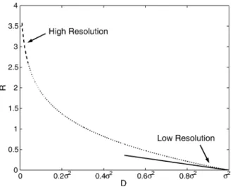
Fig. 1. The dotted line is a qualitative representation of the operational rate-distortion curve of scalar quantization. The dashed line indicates the section of the curve that is well described by (1). The solid line, which shows the tangent of thecurveatD = , indicates the low resolution performance given by (2).
accurate approximations to the performance of optimal entropy-con-strained scalar quantization in both the high- and low-resolution re-gions, as illustrated in Fig. 1.
It is interesting to compare the low resolution behavior ofR(D)for a given pdf to that of the Shannon rate-distortion function, denoted R(D), of a stationary memoryless source with the same pdf. Since R(D)represents the best performance attainable by any quantization technique, it must be thatR(D) R(D). It follows from this and the fact that, likeR(D),R(D) ! 0asD ! 2, that themagnitudeof theslopeofR(D)atD = 2is no larger than that ofR(D).
Wenow seefrom TableI that sincetheslopeofR(D)atD = 2 equals0for exponential and Laplacian pdfs, it must equal the slope of the Shannon rate-distortion function (because the latter could be no larger). Therefore, in the low-resolution region, scalar quantiza-tion for these pdfs is asymptotically as good as any quantizaquantiza-tion tech-nique—scalar, vector or otherwise. In contrast, in the high-resolution region,R(D)exceedsR(D)by 12log2e6 = 0:255bits/sample, for all pdfs.
For theuniform pdf, theslopeof R(D) atD = 2 is infinite, whereas the slope ofR(D)is finite (because it is convex). Therefore, for the uniform pdf at low rate, uniform scalar quantization is nowhere near as good as the best high-dimensional vector quantizers.
For theGaussian pdf, therate-distortion function is R(D) = 1
2log2 D. Interestingly, asD ! 2, this approaches 0 with precisely thesameslopeas R(D). Therefore, just as for exponential and Laplacian pdfs, in thelow-resolution region scalar quantization for a Gaussian pdf is asymptotically as good as any quantization technique. Weconcludethis introduction with a few additional comments. To derive the low resolution slope for a Gaussian pdf, we focus on uniform threshold quantizers with infinitely many cells, optimal reconstruction levels, and increasingly large step sizes1. While it is easy to see that, under ordinary conditions, distortionD 2and quantizer output en-tropyH 0when1is large, the slope at whichHapproaches0as D ! 2 is not obvious. Nevertheless, we find accurate approxima-tions toDandHfrom which thelow resolution slopecan bestraight-forwardly determined.
Whereas the high-resolution formula (1) is based on the fact that the source density can be approximated by a constant on most suffi-ciently small cells, the low-resolution formula (2) is based on the fact that when the cells are large, the tail of the source probability density decays sufficiently quickly that only a few cells contribute materially
to distortion and rate. We will show precisely which cells dominate the distortion and theentropy.
Wealso analyzebinary quantization and show that it has low res-olution performance characterized by the same slope. Thus, it, too, is asymptotically as good in thelow-resolution region as any quantization technique for the Gaussian memoryless source.
As Laplacian and Gaussian arethetwo most commonly cited models for transform components (usually called coefficients) [13, pp. 215–218], [14, p. 564], thefact that scalar quantization is asymp-totically as good for them as any type of quantization in the low resolution region has interesting ramifications for transform coding. In particular, in situations where transform coding is most effective, a sizable fraction of the coefficients must be coded at low rate. For such coefficients, simple scalar quantization is essentially as effective as any more sophisticated quantization technique. In contrast, to encode the coefficients that must be encoded with high resolution, scalar quantization requires approximately one quarter bit per sample more than optimal vector quantization.
We note that scalar quantization with fixed-rate coding does not at-tain the rate-distortion performance described in (2). This is because with fixed-rate coding, the smallest nonzero rate is at least1, which implies that for anyD < 2, the least rate of any fixed-rate scalar quan-tizer with mean-squared errorDor less is at least1. Consequently, the discussion throughout the correspondence is relevant to variable-rate coding, i.e., scalar quantization with entropy coding.
For completeness, we mention other analytical results on low-rate quantization of which we are aware. In [15], [16], the low resolution performance of fixed-rate transform codes is analyzed for Gaussian sources with memory, where low rate is attained with large block lengths. In [17], [18], upper bounds are found to the mean-squared error of dithered scalar quantization. Since these apply to all rates, they also apply to low rates. However, they have little use at asymptotically low rates, and in particular they give no indication of the slope of R(D)atD = 2.
Finally, we note that the method used in this correspondence applies more widely. Specifically, as shown in [19] it can also be used for a Gaussian source with absolute error distortion measure as well as to a Laplacian source with both absolute and squared error distortion mea-sures (the latter has been derived in a different way in [1]).
The remainder of the correspondence focuses on Gaussian sources and squared error distortion measure. Section II introduces and ana-lyzes uniform scalar quantization. Section III does the same for binary quantizers. Section IV offers concluding remarks. Finally, proofs of certain lemmas are relegated to the Appendix , whereas the key results are proved in Sections II and III.
II. UNIFORMTHRESHOLDQUANTIZERS
An infinite-level uniform threshold scalar quantizer (UTQ) with step size1and offset0 < 1is a scalar quantizer with partition having cellsSk= [(k0)1; (k+10)1),k 2 , along with reconstruction levelsrk 2 Sk,k 2 . Its quantization ruleisq(x) = rk, when x 2 Sk. Theoffsetindicates the fraction of cellS0that lies to the left of the origin. For example, when = 1=2, cellS0 is centered at the origin, whereas when = 0, cellS0begins at the origin. Let
1 0 .
Weassumethroughout that thesourceto bequantized is stationary, memoryless and Gaussian with mean zero and variance2, denoted N (0; 2)for short, (ordinarily we do not mention stationarity or mem-orylessness). The (output) entropy of this quantizer on such a source is
H(; 1; 2) = 0 1 k=01
wherePkdenotes the probability of thekth cell, and all logarithms in this correspondence have base2. Sincethesourceis Gaussian
Pk= Q (k 0 )1 0 Q (k + 1 0 ) 1 whereQ(x) = x1p1
2e0 dt. The mean-squared error of this quan-tizer on such a source is
d(; 1; 2) = 1
01(x 0 q(x)) 2f(x) dx
wheref is the Gaussian density. Except where stated otherwise, we take the reconstruction levels to be the centroids of their respective cells; i.e.,rk= S xf(x)P dx. As is well known, this choice minimizes distortion for a given partition. The operational rate-distortion function of infinite-level uniform threshold quantization is the function
RU; (D) = inf
0<1;1>0:d(;1; )DH(; 1;
2) (3) which specifies the least entropy of any such quantizer with mean-squared errorDor less. LetR (D) = 12logD denote the Shannon rate-distortion function of the source.
Weset to betheratio 1= and refer to it throughout as the normalized step size. We notice thatPkdepends only onand, and for emphasis, we will sometimes denote itPk(; ). Consequently, H(; 1; 2) = H(; 1=; 1), depends only on and as well. Therefore, we will frequently use the notation H(; ). Similarly, d(; 1; 2) = 2d(; 1=; 1) = 2d(; ; 1). It follows from these remarks thatRU; (D) = RU;1 D .
To find theslopeofRU; (D)atD = 2we need to consider what happens when2d(; ; 1) ! 2 andH(; ) ! 0. Weobserve that in order for the latter to happen it is necessary and sufficient that ! 1and ! 1. Moreover, because of this, for sufficiently largevalues ofD, it suffices to restrictto be greater than0in the definition ofRU; (D)in (3).
Sections II-A and II-B find asymptotic low-resolution formulas for H(; )and 2 0 d(; 1; 2), respectively, and Section II-C uses these to find an asymptotic expression forRU; (D)asD ! 2.
Before proceeding, we introduce notation and facts to be used later. LetG(x) = p1
2e0 denote the Gaussian density with mean zero and unit variance. Let the entropy function be defined as
H(. . . ; z01; z0; z1; . . .) = 0 1 k=01
zklog zk
where0 < zk 1for allkarea finiteor countably infiniteset of numbers that need not sum to one. Letox!1denote a quantity that converges to zero asx ! 1. More generally, letox!x ;y!y denote a quantity that converges to zero asx ! xoandy ! yo, where it will be clear from context whetherx % xo,x & xoor simplyx ! xo, and similarly for thevariabley. If this quantity depends on parameters other thanxandy, its convergence to zero is uniform in such parameters. To keep notation short, we writeoxinstead ofox!1, whenxo= 1, and weletox;ydenoteox!1;y!1.
The following facts provide elementary bounds and approximations to theQfunction and closely related functions.
Fact 1: Q(x) 2G(x),x 0. Fact 2: Q(x) < x1G(x),x > 0. Fact 3: Q(x) > 1x(1 0x1) G(x),x > 0. Fact 4: Q(x) > 2x1 G(x); x p 2 Q(p2); x <p2. Fact 5: Q(x) = 1xG(x) 1 + ox ,x > 0. Fact 6: Q((x + 1)) = Q(x) o,x 0; i.e., Q((x+1))Q(x) ! 0 as ! 1, uniformly forx 0.
Fact 7: For all sufficiently large,Q (x + 1) < 12Q(x)for allx 0.
Fact 8: For all sufficiently large,
Q(x) 0 Q((x + 1)) > 4x1 G(x); x p 2 Q(p2) 2 ; 0 x < p 2: Fact 9: C(x) x1t G(t) dt = G(x). Fact 10: V (x) 1 x t 2G(t) dt = x G(x) + Q(x) = x G(x) [1 + ox]: Fact 11: C((x + 1)) = C(x) o,x 0; i.e., C((x+1))C(x) ! 0 as ! 1, uniformly forx 0. Fact 12: V ((x + 1)) = V (x) o,x 0; i.e., V ((x+1))V (x) ! 0 as ! 1, uniformly forx 0.
Facts 1, 2, and 3 are demonstrated in [20, pp. 82–83]. Fact 4 truncates thelower bound of Fact 3. Fact 5 follows from Facts 2 and 3. Fact 6 is derived by upper bounding Q((x+1))Q(x) using Facts 1 and 4 when x < p2, and using Facts 2 and 4 whenx p2. Fact 7 follows from Fact 6, and Fact 8 follows from Facts 4 and 7. Fact 9 and the first equality of Fact 10 derive from elementary integration. The second equality of Fact 10 follows from Fact 5. Fact 11 follows from Fact 9 and simple manipulation of exponentials. Finally, Fact 12 is derived using Facts 10, 4, and 2. Specifically, whenx <p2, Fact 4 is used to lower boundV (x), and thefact thatx < p2is used to upper boundV ((x + 1)). Whenx p2, Fact 2 is used to upper bound V ((x + 1)).
A. Asymptotic Entropy
We begin with several lemmas (one is proved here and the rest are proved in the Appendix) that lead to the main result of this section, a low resolution approximation for entropy.
Lemma 1: When a UTQ with offset,0 < < 1, and sufficiently large normalized step sizeis applied to aN (0; 2)source
A: Pk+1(; ) < Pk(; )P1(; ) for alland allk 1 B: Pk01(; )<Pk(; )P01(; )for alland allk 01:
Lemma 2:
lim p!0
H(1 0 p + p op!0)
H(p) = 0:
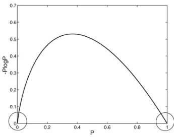
We comment that this lemma is due to the fact that the entropy func-tionH(p) = 0p log phas infiniteslopeatp = 0and finiteslope atp = 1, as illustrated in Fig. 2. A formal proof is provided in the appendix.
The next lemma shows that in low resolution, quantizer entropy is dominated by the cells adjacent to the center cell.
Lemma 3: For a UTQ with offset,0 < < 1, and normalized step sizeapplied to aN (0; 2)source
H(. . . ; P01(; ); P0(; ); P1(; ); . . .)
Fig. 2. Theentropy function,0p log p.
Proof: For brevity, we omit the parameters and from Pk(; ). The proof is composed of two main steps. In Step 1, we show that H(. . . ; P01; P0; P1; . . .) can beasymptotically approxi-mated by the three middle terms; that is,
H(. . . ; P01; P0; P1; . . .) = H P01; P0; P1 1 + o; : In Step 2, it is shown that these three terms can be asymptotically ap-proximated by only two terms; that is,
H P01; P0; P1 = H P01; P1 1 + o; where we note thatP0! 1as ! 1and ! 1.
Step 1:Wefirst show that for all sufficiently largeand, 1 < H(. . . ; PH(P01; P0; P1)01; P0; P1; . . .)< 1 + 6P1+ 6P01: (4) The left inequality is trivial. We upper bound the middle term in the following way: 1 k=010Pklog Pk 1 k=010Pklog Pk = 1 + 02 k=010Pklog Pk+ 1k=20Pklog Pk 1 k=010Pklog Pk(s) < 1 + 02k=010Pklog Pk 0P01log P01 + 1 k=20Pklog Pk 0P1log P1 : (5) Consider the terms in the last summation. We claim that when is sufficiently large,0Pklog Pk < 0P1klog P1k for allk 2. To se e this, we observe that when is large, so is(since < 1), and Lemma 1 impliesPk < Pk01P1for allk 2, which in turn implies Pk < Pk
1 < P1, for allk 2. Next, Fact 1 implies thatP1 < Q() < 1
e when is sufficiently large. Since0p log pincreases forp < 1e,0Pklog Pk < 0P1klog P1k for allk 2, when is sufficiently large. Substituting this into the last summation of (5), we havethat whenis sufficiently large
1 k=20Pklog Pk 0P1log P1 < 1 k=20P1klog P1k 0P1log P1 = 1 k=2 kPk01 1 =(1 0 P1)2P1 2 0 P12 (1 0 P1)2 <(1 0 P1)2P1 2 < 6P1
where the last inequality derives from the fact thatP1 < 1e. In much thesameway it follows that whenis sufficiently large
02
k=010Pklog Pk
0P01log P01 < 6P01:
This shows (4).SubstitutingP01 = oandP1 = ointo (4), we obtain
H(. . . ; P01; P0; P1; . . .) = H P01; P0; P1 1 + o which completes Step 1.
Step 2:Wewill show that H(P0) = H(P1; P01) o;, from which it will follow that
H P01; P0; P1 = H P01; P1 1 + o; :
DefineP = 02k=01Pk+ 1k=2Pk. Using thefact that for all suf-ficiently large,Pk < Pk01P1 for allk 2, weupper bound the second sum as 1 k=2 Pk< 1 k=2 Pk 1 = P 2 1 1 0 P1 < 2P12;
where the last inequality is due toP1< 12for all sufficiently large. Thefirst sum in thedefinition ofPcan be upper bounded in much the same way, except that it holds for all sufficiently large. Thus when andare both sufficiently large,P < 2(P012 + P12). Therefore, P0>1 0 P010 P10 2(P2
01+ P12)>1 0 P010 P10 2(P01+ P1)2: SinceP01+ P1 = o+ o, it follows that whenand are sufficiently large,P0 > 1 0 P010 P10 2(P01+ P1)2> 1e, which sinceH(p)decreases monotonically forp > 1e, implies that
H(P0) < H 1 0 P010 P10 2(P01+ P1)2 : Consequently H(P0) H P01; P1) < H(1 0 P010 P10 2(P01+ P1)2 H(P01; P1) <H 1 0 P010 P10 2(P01+ P1) 2 H(P01+ P1) = H(1 0 p 0 2pH(p) 2)
wherep P01+ P1, and where the second inequality follows from theeasy to provefact that for anya; b 2 +,H(a + b) < H(a; b). We observe that asand tend to infinity,pgoes to zero. Therefore, by Lemma 2 it follows that H(10p02p )H(p) ! 0asp ! 0. This shows thatH(P0) = H(P1; P01) o;, which completes Step 2 and the proof of thelemma.
Lemma 4: Leta(s)andb(s)bepositivefunctions on such that a(s) = b(s)[1+os], and for some" > 0,jb(s)01j > "for alls. Then
H(a(s)) = H(b(s)) 1 + os : Lemma 5:
H Q(x) = log e2 x G(x) 1 + ox :
The following theorem gives the low resolution approximation to the entropy of uniform quantization.
Theorem 6: For a UTQ with offset,0 < < 1, and normalized step sizeapplied to aN (0; 2)source
whereH(; ) = H(. . . ; P01(; ); P0(; ); P1(; ); . . .)is the quantizer entropy.
If onefixes, this theorem shows the rate at which entropy con-verges to0as ! 1. However, the convergence is not uniform in , and this theorem shows how entropy depends onas well as. In particular, it gives an accurate approximation to quantizer entropy when bothandarelarge. Noticethat = 0is not allowed since H(0; ) = 1 + o, namely, the output entropy does not go to zero as ! 1.
Proof: For brevity, we omit the parameters and from Pk(; ). Lemma 3 shows that
H(; )=H(. . . ; P01; P0; P1; . . .)=H P01; P1 1 + o; : (7) Since P01 = Q() 0 Q (1 + ) , Fact 6 implies that P01= Q()[1+o], and thus in particularP01= Q()[1+o], since0 < < 1. SincejQ() 0 1j > 12 for all, it follows from Lemma 4 thatH(P01) = H(Q()) [1 + o]. Next, applying Lemma 5, we obtain
H(Q()) = 12log e G() 1 + o : Combining these yields
H(P01) = 12log e G() 1 + o : In a similar way
H(P1) = 12log e G() 1 + o :
Combining theexpressions forH(P01)andH(P1)together with (7) completes the proof of the theorem.
We now comment on the cell or cells that dominate entropy when it is small. TheentropyH(; )will besmall if and only ifP0 1and Pk 0,k 6= 0, which makes0Pklog Pk 0for allk, and which happens if and only ifandare both large. Lemma 3 shows that H(; )is dominated by the cells,S01andS1, immediately adjacent to the center cell. This is not coincidental; rather, as mentioned earlier, it follows from the fact, illustrated in Fig. 2, that the entropy function, H(p) = 0p log p, has infiniteslopeatp = 0and finiteslopeatp = 1. Thus, when entropy is nearly zero, it is dominated by the largest of the nearly zero probabilities, which areP01and/orP1. Indeed the two terms within the large parentheses in (6) correspond toH(P01) andH(P1), respectively. If , e.g., if < 12 andis very large, thenP01 P1, and it is cellS01and thefirst term within the parentheses that dominate the entropy. Conversely, if , then P1 P01, and it is cellS1and the second term within the parentheses that dominate. Finally, if , then the two dominating cells contributeroughly thesameto theentropy.
B. Asymptotic Distortion
The following theorem provides the low-resolution approximation to distortion.
Theorem 7: For a UTQ with offset,0 < < 1, normalized step size, centroid reconstruction levels, and aN (0; 2)source
20 d(; 1; 2)
2 = G() + G() 1 + o; :
Like Theorem 6, this theorem gives an accurate approximation when bothand are large. The proof will be structured in a way that makes evident which cell or cells dominate20 d(; 1; 2).
Proof: For brevity we omit the arguments ofd(; 1; 2). Le t 2
k
S x
2f(x) dx = 2 V ((k 0 )) 0 V ((k + 1 0 )) where f is thepdf of theGaussian sourceand V (x) is defined in Fact 10. Let
dk
S (x 0 rk)
2f(x) dx = 2 k0 r2kPk
bethecontribution of thekth cell to the distortion (recalling that rk = S xf(x) P dx). Weobservethat2 = k2kandd = kdk. Wenow write 20 d = 20 d0 0 d010 d10 jkj2 dk: (8)
We deal with these terms in reverse order. First, sincedk k2
jkj2 dk jkj2 k2= 0(+1)1 01 x 2f(x) dx+ 1 (20)1x 2f(x) dx = 2V (( + 1)) + 2V ((2 0 )) (a) = 2V () o+ 2V ((1 0 )) o (b) = 2 G() o+2 G() o (9)
where(a)follows from Fact 12, and(b)is obtained using Fact 10. Next, wehave(10) shown at thebottom of thepage, where(a)is due to thedefinition ofC(x)given in Fact 10,(b)follows from Facts 6, 11, and 12, and(c)follows from Facts 5, 9, and 10. By symmetry it follows that d01= 2 G() o: (11) Finally 20 d0= (20 2 0) + (020 d0) (12) where as in (9) above 20 2 0 = k6=0 2 k= 2V () + 2V ((1 0 ) = 2G() 1 + o + 2G() 1 + o (13) d1= 2 10 r21P1 (a) = 2(V ((1 0 )) 0 V ((2 0 ))) 0 C((1 0 )) 0 C((2 0 ))Q((1 0 )) 0 Q((2 0 )) 2 Q((1 0 )) 0 Q((2 0 )) (b)= 2V ((1 0 )) 1 + o 0 2 C((1 0 )) 1 + o 2 Q (1 0 ) 1 + o (c)= 2 G() [1 + o] 0 2G2() 1 + o 1 G() 1 + o = 2 G() o (10)
where the third equality uses Fact 10, and where as in (10) 2 00 d0 = r20P0 = 1 0 Q() 0 Q((1 0 ))C() 0 C((1 0 )) 2 1 0 Q() 0 Q() (a) = 2 G() 0 G() 2 1 + o+ o = 2 G() G() 0 G() +G() G()0G() 1 + o+ o (b)= 2 G()o+ G()o 1 + o+ o = 2 G() + 2 G() o; (14)
where(a)is dueto Fact 9, and(b)follows from having
G() 0 G() = G() 0 G() = o
and similarly
G() 0 G() = o:
Substituting (13) and (14) into (12) yields
20 d0= 2 G() + 2 G() 1 + o;
: (15) Substituting (9), (10), (11), and (15) into (8) yields
20 d = 2 G() + G() 1 + o;
:
Dividing theaboveby2gives the desired result.
We now consider which cell or cells make the dominating contribu-tion to20d, when the latter is very small. Whend 2, bothand are large. From (15), we see thatd0 2, and from (9)–(11), we see thatdk 0fork 6= 0. We are interested, however, in finding the cells that dominate the rate at which distortion converges to variance. Sinced0! 2anddk! 0,k 6= 0, it makes most sense to compare 20 d0and thesum of thedk’s,k 6= 0. Comparing (15) to (9)–(11), reveals that k6=0dkis asymptotically negligible relative to20 d0. Weconcludethat whend 2,20 d0is thedominant component of20 d.
C. Asymptotic Rate-Distortion
The following lemma, which is used in the proof of Theorem 9 below, derives directly from Theorems 6 and 7.
Lemma 8: For a UTQ with offset,0 < < 1, normalized step size, centroid reconstruction levels, and aN (0; 2)source
H(; )
20 d(; 1; 2) = log e22 1 + o; The following is the principal result of this correspondence.
Theorem 9: In the low resolution region, the operational rate-dis-tortion function of infinite-level uniform threshold scalar quantization for a Gaussian sourcewith variance2is
RU; (D) = log e2 1 0 D2 1 + o : (16)
Proof: SinceRU; (D) = RU;1 D , it suffices to show lim
D!1
RU;1(D)
1 0 D = log e2 : (17)
Next, we rewrite the operational rate-distortion function for a unit vari-ancesourcefor all sufficiently largeDas
RU;1(D) = inf
0<<1RU;1;(D) where
RU;1;(D) inf
1>0:d(;1;1)DH(; 1)
is the operational rate-distortion function of UTQ with fixed offset for a source with unit variance, and as mentioned before, = 0can be omitted from the constraint sinceDis sufficiently large. As a prelim-inary to showing (17), wewill showRU;1;(D)satisfies (17) for any fixed 2 (0; 1). First lim sup D!1 RU;1;(D) 1 0 D (a) = lim sup !1 RU;1; d(; ; 1) 1 0 d(; ; 1) (b) lim sup !1 H(; ) 1 0 d(; ; 1) (c)= log e 2 (18)
where(a)derives from the fact thatd(; ; 1)goes continuously to1 as ! 1,(b)follows from thedefinition ofRU;1; d(; ; 1) , and (c)is obtained from Lemma 8. Next
lim inf D!1 RU;1;(D) 1 0 D (a) lim inf !1 H(; ) 1 0 d(; ; 1) (b)= log e 2 (19)
where(b)is obtained from Lemma 8 and(a)is shown as follows. By thedefinition of RU;1;(D), for anyD 2 (0; 1), there exists(D) such that
H(; (D)) RU;1;(D) + "(D) and d(; (D); 1) D (20) where"(D) > 0andlimD!1"(D)10D = 0. (Thechoices of"(D)and (D)are not unique, but any fixed choices will do.) From (18) it fol-lows thatRU;1;(D) ! 0asD ! 1. Thus, by (20)H(; (D)) ! 0 asD ! 1, which implies that(D) ! 1as D ! 1, since H(; ) ! 0if and only if ! 1. This and (20) yield
lim inf D!1 RU;1;(D) 1 0 D lim infD!1 H(; (D)) 0 "(D) 1 0 d(; (D); 1) lim inf !1 H(; ) 1 0 d(; ; 1): It now follows from (18) and (19) that
lim D!1
RU;1;(D)
Finally, to obtain the result of the theorem we proceed as follows: lim sup D!1 RU;1(D) 1 0 D (a) = lim sup D!1 infRU;1;(D) 1 0 D (b) inf lim supD!1 RU;1;(D) 1 0 D (c) = log e2 (22)
where(a)follows from thedefinition ofRU;1(D),(b)is elementary, and(c)follows from (21). Similarly
lim inf D!1 RU;1(D) 1 0 D (a) lim inf D!1 R1(D) 1 0 D (b)= lim inf D!1 1 2logD1 1 0 D (c) = log e2 (23)
whereR1(D)is theShannon rate-distortion function of a unit variance Gaussian source, and where(a)follows from the converse rate-dis-tortion theorem,(b)uses the well-known formula forR1(D)[21, p. 477], and(c)is obtained by taking the limit, for example, by using L’Hospital’s rule. Equation (17) and the theorem now follow from (22) and (23). We note that (19) could have been shown using Shannon’s rate-distortion function as a lower bound, as was done in (23). How-ever, the approach taken above, demonstrates that
lim D!1 RU;1;(D) 1 0 D = lim!1 H(; ) 1 0 d(; ; 1)
without using either Gaussianity or Shannon’s rate-distortion function. It requires only that the latter limit exist.
As it is easy to see, R (D) = 12log
2
D = log e2 1 0 D2 1 + o : Comparing this to the theorem statement reveals that for a Gaussian source and the low resolution region, the operational rate-distortion function of infinite-level uniform threshold scalar quantization and the Shannon rate-distortion function approach0with thesameslopeas D ! 2. Therefore, in the low resolution region, such quantizers areasymptotically as good as any quantization technique— scalar, block, or otherwise. Additionally, from (21) and the relation between RU; ;(D)andRU;1;(D), oneconcludes that for any 6= 0, the operational rate-distortion functionRU; ;(D)of uniform threshold quantization with offsetalso approaches zero with the same slope as the Shannon rate-distortion function, as does the operational rate-dis-tortion function of scalar quantization in general. Finally, we note that from the dominance results presented previously, the slope is approx-imately equal toH(P 0D)+H(P ), i.e., the distortion term is dominated by the center cell and the entropy is dominated by the two adjacent cells.
Remark: We assumed throughout that the quantizers’ reconstruc-tion levels were centroids, which is necessary for optimal performance. It turns out, however, that this assumption can be relaxed somewhat, asymptotically in the low-resolution region. That is, for Theorem 9 to hold it is only necessary that the reconstruction levels be sufficiently close to the centroids. More specifically, there is very little sensitivity
to the reconstruction levels fork 6= 01; 0; 1, in thesensethat there-quirement thatrk2 Skis sufficient. Fork = 01; 0; 1, the requirement depends on the behavior ofrelative toas both quantities tend to infinity. If , thenr01needs to be close to the centroid ofS01 and there is no restriction onr1(except for lying inS1). Similarly, if , thenr1 needs to be close to the centroid ofS1and there is no restriction onr01(except for lying inS01). Lastly, if , then bothr01andr1need to be close to the centroids ofS01andS1, respectively. In all cases,r0 needs to be sufficiently close to zero. A formal derivation of these statements can be found in [22, pp. 98–104].
III. BINARYQUANTIZERS
A binary (two-level) scalar quantizer is characterized by three num-bers: a thresholdtand two reconstruction levelsr0< tandr1 t. Le t S0(t) = (01; t)andS1(t) = [t; 1)bethetwo quantization cells, and let the quantization rule beq(x) = rkwhenx 2 Sk,k = 0; 1.
As in the previous section, the source considered is stationary, mem-oryless Gaussian with mean zero and variance2, and thereconstruc-tion levelsr0andr1are taken to be the cell centroids, unless otherwise specified. We letPkorPk(t; 2)denotetheprobability of thesource valuelying inSk,k = 0; 1.
LetH(t; 2) = H(P0(t; 2); P1(t; 2))denote the entropy of the quantizer output with thresholdtfor the Gaussian source. Let
d(t; 2)1= 1
01(x 0 q(x)) 2f(x) dx
denote the mean-squared error distortion of this quantizer on this source. The operational rate-distortion function of binary quantization for this sourceisRB; (D) = inft:d(t; )DH(t; 2), which spec-ifies the least entropy of any such quantizer with mean-squared error Dor less.
It is easy to see thatPk(t; 2) = Pk(t; 1),H(t; 2) = H(t; 1), d(t; 2) = 2d(t
; 1), andRB; (D) = RB;1(D). Hence it is con-venient to parameterizePkandHby = t, i.e.,Pk()andH(). Due to the symmetry of the Gaussian density, it suffices to restrict at-tention tot > 0.
As before, we will find asymptotic low-resolution approximations to entropy and distortion, and then combine these to determine the asymptotic low resolution expression forRB; (D). We also deter-mine which cells dominate entropy and distortion, and we relax the requirement that the levels be centroids. Since the derivations in the binary casearesimilar in spirit to thosein theuniform case, wewill only state the results and provide no proofs, so as to spare the reader repetitive details.
Theorem 10: For a binary scalar quantizer with thresholdtapplied to aN (0; 2)source
H() = log e2 G() 1 + o ;
where as indicated earlier = t,H() = H(P1(); P2())and G(x)denotes a zero-mean, unit-variance Gaussian density.
Theorem 11: For a binary scalar quantizer with thresholdtand re-construction levels at cell centroids applied to aN (0; 2)source
20 d(t; 2)
2 = G() 1 + o
Theorem 12: In the low resolution region, the operational rate-dis-tortion function of binary scalar quantization for a Gaussian sourcewith variance2is
RB; (D) = log e2 1 0 D2 1 + o :
Notice that the expression given in this theorem for binary quantiza-tion is precisely the same as that given in Theorem 9 for infinite-level uniform threshold quantization, which in turn matches the Shannon rate-distortion function in the low resolution region. We conclude that binary quantization is another type of quantization that is asymptoti-cally optimal in thelow resolution region.
We now comment on the cells that dominate the entropy and distor-tion. As before, when entropy is small, it is dominated by the cell that has largest probability not close to one, which isS1. And just as with uniform quantizers, when distortion is close to2,20 Dis domi-nated by the cell whose probability is nearly one, namely,S0. That is,
0D 0D 1.
As with uniform quantizers, the requirement for cell centroids can be relaxed somewhat. Specifically, the reconstruction levels need not lie exactly at cell centroids, but they do need to be sufficiently close to them. This is formally stated in [22, pp. 106–107].
IV. CONCLUSION
This correspondence considered the asymptotic performance of scalar quantizers in the low-resolution domain, which is determined by the slope of the operational rate-distortion function of such quantizers at distortion equal 2. For the cases of exponential, Laplacian and uniform sources and difference distortion measures, this slope has been provided in or can be determined from [1], [2]. The focus of this correspondence has been on the Gaussian source and squared error distortion measure. We considered infinite-level uniform threshold and binary scalar quantizers in the asymptotic case that the cell sizes tend to infinity (for the uniform case) and that the quantizer threshold tends to infinity (for the binary case). We derived simple formulas for the rate of convergence of entropy to zero and of mean-squared error distortion to thesourcevariance.
The convergence of entropy and distortion as ! 1for uniform quantization is not uniform in theoffset. The derived formulas show how entropy and distortion depend onas well as. Specifically, they provideaccurateapproximations when bothandarelarge.
Using these convergence formulas, the operational rate-distortion function of infinite-level uniform threshold and binary scalar quanti-zation has been shown to approach zero asD ! 2with thesame slopeas that of theShannon rate-distortion function. This shows that in thelow resolution region scalar quantization (in particular uniform and binary) is asymptotically optimal for Gaussian sources and squared error distortion measure.
Last, the method used in this correspondence can also be applied to a Gaussian source with absolute error distortion measure and to a Laplacian source with both absolute and squared error distortion mea-sures [19].
APPENDIX
A. Proof of Lemma 1
Wewill show Part A; PartB follows by symmetry. To simplify notation, we omit the parametersandfromPk(; ). Consider k 1. First, Fact 8, with(k 0 ) playing theroleofx, shows that
for all sufficiently large , thefollowing lower bound toPk holds for all k 1: Pk= Q (k 0 ) 0 Q (k + 10) > 1 4(k0)1 G((k0)); (k 0 ) p 2 (a) Q(p2) 2 ; (k 0 ) < p 2 (b): (A1) Next, we upper boundPk+1using Fact 2
Pk+1= Q (k + 1 0 ) 0 Q (k + 2 0 ) <(k + 1 0 )1 G((k + 1 0 )):
Combining thelower bound toPkwith theupper bound toPk+1, we obtain Pk+1 Pk < 4e 0 ; (k 0 ) p2 (a) 2 G((k+10)) Q(p2)(k+10); (k 0 ) < p 2 (b): (A2)
It now suffices to show that for all sufficiently large, theabove upper bound to PP is smaller than the lower bound toP1 obtained from (A1). We do so by considering two cases.
Case 1: (k 0 ) <p2—In this case,(1 0 ) <p2. Thus, by (A1b),P1 > Q( p 2) 2 . Next, by (A2b), Pk+1 Pk < 2 G((k + 1 0 ))Q(p2)(k + 1 0 ) < 2 G()Q(p2) where the last inequality usesk + 1 0 > 1. SinceP1> Q(
p 2) 2 and P
P < Q(2 G()p2) ! 0as ! 1, weconcludethat for all sufficiently large,PP < P1, for allk; such that(k 0 ) <p2.
Case 2: (k 0 ) p2— We consider two subcases. First, sup-pose(1 0 ) <p2. Then by (A1b),P1 >Q(
p 2)
2 . Next, by (A2a) Pk+1
Pk < 4e0 < 4e0 :
Weconcludethat for all sufficiently large,PP < P1, for all of the k; such that(k 0 ) p2and(1 0 ) <p2. Next, suppose (1 0 ) p2. Then by (A1a) P1> 14(1 0 )1 G((1 0 )) > 141G() using1 0 < 1. By (A2a) Pk+1 Pk < 4e0 < 4e0 e0 p 2 using(k 0 ) p2. Sincee0 p 2 ! 0faster than 1 ! 0, we concludethat for all sufficiently large, PP < P1, for allk; such that(k 0 ) p2and(1 0 ) p2. This completes the proof of PartAand thelemma.
B. Proof of Lemma 2
We need to show that
lim p!0
0(1 0 p + p op!0) ln (1 0 p + p op!0)
0p ln p = 0:
Thefact thatlimx!0ln(10x)0x = 1, or equivalently, that ln(10x)0x = 1 + ox!0, implies
0(1 0 p + p op!0) ln (1 0 p + p op!0) 0p ln p
= 0(1 0 p + p o(1 0 p + p op!0)(p + p op!0)p!0) ln (1 0 p + p op!0) 1 (1 0 p + p o0p ln pp!0)(p + p op!0)
= 1 + op!0 1 10 p +p op!0 1+op!0]0ln p 0!0asp ! 0
which proves the lemma.
C. Proof of Lemma 4 It is sufficient to show lim s!s H(a(s)) H(b(s)) = 1: We have the following string of equalities:
H(a(s))
H(b(s)) = 0a(s) log a(s)0b(s) log b(s) = a(s)b(s)
log a(s) b(s)b(s) log b(s) = a(s)b(s) 1 +log a(s) b(s) log b(s) = a(s)b(s) + a(s) b(s)loga(s)b(s) log b(s) :
Sincejb(s)01j > "for alls, it follows that eitherlog b(s) > log(1+") orlog b(s) < log(10")for alls. Therefore,log b(s)is bounded away from zero. Combining this with the fact thata(s)b(s) ! 1ass ! 1, and thata(s)b(s)loga(s)b(s) ! 0ass ! 1, theresult follows.
D. Proof of Lemma 5
The lemma is obtained by using Fact 5 in the first equality as follows: H Q(x) = H 1xG(x) 1 + ox = 0 1xG(x) 1 + ox log 1xG(x) 1+ox = 1 xG(x) 1+ox log p 2x+ x2
2 log e0log 1+ox = log e2 x G(x) 1 + ox :
REFERENCES
[1] G. J. Sullivan, “Efficient scalar quantization of exponential and Lapla-cian random variables,”IEEE Trans. Inf. Theory, vol. 42, no. 5, pp. 1365–1374, Sep. 1996.
[2] A. Gyorgy and T. Linder, “Optimal entropy-constrained scalar quanti-zation of a uniform source,”IEEE Trans. Inf. Theory, vol. 46, no. 7, pp. 2704–2711, Nov. 2000.
[3] A. Gersho and R. M. Gray,Vector Quantization and Signal Compres-sion. Boston, MA: Kluwer, 1992.
[4] T. Berger, “Optimum quantizers and permutation codes,”IEEE Trans. Inf. Theory, vol. IT-18, no. 6, pp. 759–765, Nov. 1972.
[5] A. N. Netravali and R. Saigal, “Optimal quantizer design using a fixed-point algorithm,”Bell Syst. Tech. J., vol. 55, pp. 1423–1435, Nov. 1976. [6] P. Noll and R. Zelinski, “Bounds on quantizer performance in the low bit-rateregion,”IEEE Trans. Commun., vol. COM-26, no. 2, pp. 300–305, Feb. 1978.
[7] N. Farvardin and J. W. Modestino, “Optimum quantizer performance for a class of non-Gaussian memoryless sources,”IEEE Trans. Inf. Theory, vol. IT-30, no. 3, pp. 485–497, May 1984.
[8] J. C. Kieffer, T. M. Jahns, and V. A. Obuljen, “New results on optimal entropy-constrained quantization,”IEEE Trans. Inf. Theory, vol. 34, no. 5, pp. 1250–1258, Sep. 1988.
[9] P. A. Chou, T. Lookabaugh, and R. M. Gray, “Entropy-constrained vector quantization,”IEEE Trans. Acoust., Speech, Signal Process., vol. 37, no. 1, pp. 31–42, Jan. 1989.
[10] J. Buhmann and H. Kuhnel, “Vector quantization with complexity costs,”IEEE Trans. Inf. Theory, vol. 39, no. 4, pp. 1133–1145, Jul. 1993.
[11] K. Rose and D. Miller, “A deterministic annealing algorithm for en-tropy-constrained vector quantizer design,” inProc. Asilomar Conf. Sig-nals, Systems, and Computing, vol. 2, Pacific Grove, CA, Nov. 1993, pp. 1651–1655.
[12] H. Gish and J. N. Pierce, “Asymptotically efficient quantization,”IEEE Trans. Inf. Theory, vol. IT-14, no. 5, pp. 676–683, Sep. 1968. [13] A. N. Netravali and B. G. Haskell,Digital Pictures: Representation,
Compression and Standards, 2nd ed. New York: Plenum, 1988. [14] N. S. Jayant and P. Noll,Digital Coding of Waveforms: Principles and
Applications to Speech and Video. Englewood Cliffs, NJ: Prentice-Hall, 1988.
[15] D. F. Lyons and D. L. Neuhoff, “A coding theorem for low-rate trans-form codes,” inProc. IEEE Int. Symp. Information Theory, San Antonio, TX, Jan. 1993, p. 333.
[16] D. F. Lyons, “Fundamental Limits of Low-Rate Transform Codes,” Ph.D. dissertation, EECS Dept., Univ. Michigan, Ann Arbor, 1992. [17] J. Ziv, “On universal quantization,”IEEE Trans. Inf. Theory, vol. IT-31,
no. 3, pp. 344–347, May 1985.
[18] R. Zamir and M. Feder, “On universal quantization by randomized uni-form/latticequantizers,”IEEE Trans. Inf. Theory, vol. 38, no. 2, pp. 428–436, Mar. 1992.
[19] D. Marco and D. L. Neuhoff, “Low Resolution Scalar Quantization for Gaussian and Laplacian Sources with Absolute and Squared Error Dis-tortion Measures,” Univ. Michigan, Ann Arbor, CSPL Tech. Rep., TR 372, Jan. 2006.
[20] J. M. Wozencraft and I. M. Jacobs,Principles of Communication Engi-neering. New York: Wiley, 1967.
[21] R. G. Gallager, Information Theory and Reliable Communication. New York: Wiley, 1968.
[22] D. Marco, “Asymptotic Quantization and Applications to Sensor Net-works,” Ph.D. dissertation, EECS Dept., Univ. Michigan, Ann Arbor, 2004.