Intelligent Medium Access Control
Protocols for Wireless Sensor
Networks
Yan Yan
Ph.D.
University of York
Electronics
May 2015
Abstract
The main contribution of this thesis is to present the design and evaluation of intelligent MAC protocols for Wireless Sensor Networks (WSNs). The objective of this research is to improve the channel utilisation of WSNs while providing flexibility and simplicity in channel access. As WSNs become an efficient tool for recognising and collecting various types of information from the physical world, sensor nodes are expected to be deployed in diverse geographical environments including volcanoes, jungles, and even rivers. Consequently, the requirements for the flexibility of deployment, the simplicity of maintenance, and system self-organisation are put into a higher level. A recently de-veloped reinforcement learning-based MAC scheme referred as ALOHA-Q is adopted as the baseline MAC scheme in this thesis due to its intelligent collision avoidance feature, on-demand transmission strategy and relatively simple operation mechanism. Previous studies have shown that the reinforcement learning technique can consider-ably improve the system throughput and significantly reduce the probability of packet collisions. However, the implementation of reinforcement learning is based on as-sumptions about a number of critical network parameters. That impedes the usability of ALOHA-Q. To overcome the challenges in realistic scenarios, this thesis proposes numerous novel schemes and techniques. Two types of frame size evaluation schemes are designed to deal with the uncertainty of node population in single-hop systems, and the unpredictability of radio interference and node distribution in multi-hop systems. A slot swapping techniques is developed to solve the hidden node issue of multi-hop networks. Moreover, an intelligent frame adaptation scheme is introduced to assist sensor nodes to achieve collision-free scheduling in cross chain networks. The com-bination of these individual contributions forms state of the art MAC protocols, which offers a simple, intelligent and distributed solution to improving the channel utilisation and extend the lifetime of WSNs.
Contents
Abstract . . . ii
List of Figures . . . vii
List of Tables . . . x
Acknowledgements . . . xi
Declaration . . . xii
1 Introduction 1 1.1 Research Background . . . 1
1.2 Overview of Medium Access Control Layer . . . 4
1.3 Overview of Reinforcement Learning Technique . . . 5
1.3.1 Q-learning . . . 8
1.4 The Scope of Thesis . . . 11
1.5 Thesis Outline . . . 13
2 Fundamentals of Wireless Sensor Networks 16 2.1 A Brief History of Wireless Sensor Networks . . . 17
2.2 System Classification . . . 18
2.3 Sensor Node Technology . . . 20
2.3.1 Basic Functionalities . . . 20
2.3.2 Node Architecture . . . 23
2.4 Communication Protocol Stack . . . 26
2.5 Current Applications . . . 28
2.5.1 Environmental Application: Habitat Monitoring . . . 28
2.5.3 Health Application: Wearable Medical Sensors . . . 31
2.5.4 Summary . . . 32
2.6 Design Challenges . . . 33
2.7 Summary . . . 36
3 Medium Access Control Protocols 37 3.1 Fundamentals of MAC protocols . . . 38
3.1.1 Introduction . . . 38
3.1.2 MAC Design Trade-offs . . . 40
3.1.3 Energy Efficiency of MAC Design . . . 43
3.1.4 Taxonomy of MAC Protocols . . . 44
3.2 Examples of MAC protocols . . . 51
3.2.1 Pure ALOHA protocol . . . 51
3.2.2 Slotted ALOHA protocol . . . 53
3.2.3 Sensor-MAC protocol: S-MAC . . . 54
3.2.4 Timeout MAC protocol: T-MAC . . . 56
3.2.5 Zebra MAC protocol: Z-MAC . . . 58
3.2.6 IEEE 802.15.4 MAC layer . . . 58
3.3 ALOHA-Q . . . 62
3.4 Summary . . . 64
4 Simulation Techniques and Validation Methods 66 4.1 Introduction . . . 66
4.2 Discrete Event Simulation . . . 67
4.3 OPNET Modeller . . . 68
4.4 Performance Measures and System Assumptions . . . 73
4.5 Validation Methods . . . 76
4.6 Summary . . . 76
5 Frame Size Adaptation of ALOHA-Q for Single-hop WSNs 77 5.1 Introduction . . . 78
5.2 Modelling of ALOHA-Q in Single-hop Network . . . 79
5.2.1 Scenarios and Parameters . . . 79
5.2.2 Traffic Model . . . 81
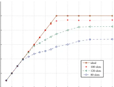
5.3 Impact of Frame Size Selection on Performance of ALOHA-Q . . . . 82
5.3.1 Throughput Performance . . . 84
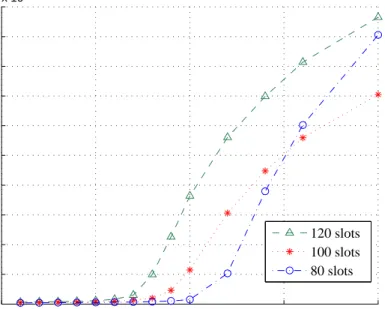
5.3.2 Delay Performance . . . 86
5.3.3 System Convergence Time . . . 87
5.4 Distributed Frame Size Adaptation . . . 88
5.4.1 Basic Principle . . . 88
5.4.2 Frame Size Adaptation Process . . . 90
5.4.3 Consistency of Frame Size Adjustment . . . 92
5.5 Performance Analysis . . . 95
5.6 Summary . . . 100
6 A Self-adaptive ALOHA-Q Protocol for Multi-hop WSNs 101 6.1 Introduction . . . 102
6.2 Network Topologies . . . 102
6.2.1 Linear Chain Topology . . . 103
6.2.2 Cross Chain Topology . . . 106
6.3 Adaptation of ALOHA-Q to Linear Chain Networks . . . 107
6.3.1 Maximum Throughput and Optimal Frame Size Estimation . . 107
6.3.2 Actual Throughput Analysis . . . 110
6.3.3 Hidden Node Problem . . . 114
6.3.4 Slot Swapping Technique . . . 117
6.3.5 Frame Size Adaptation for Linear Chain Networks . . . 120
6.3.6 Performance Analysis . . . 124
6.4 Adaptation of ALOHA-Q to Cross Chain Networks . . . 127
6.4.1 Subframe Adaptation Scheme for Cross Chain Networks . . . 127
6.4.2 Performance Analysis . . . 131
7 Future Work 138
7.1 Frame Size Adaptation to Event-based Traffic Delivery . . . 138
7.2 Intelligent Duty Cycling . . . 139
7.3 Lifelong Machine Learning . . . 139
8 Summary and Conclusions 141 8.1 Novel Contributions . . . 143
8.1.1 Frame Size Adaptation for Single-hop Networks . . . 143
8.1.2 Adaptation of ALOHA-Q to Linear Chain Networks . . . 144
8.1.3 Subframe Adaptation . . . 144
8.2 Publications . . . 145
Glossary 146
List of Figures
1.1 Protocol Stack of WSNs . . . 5
1.2 Reinforcement Learning Process . . . 6
1.3 Example of Q-learning . . . 10
1.4 Simplified Environment . . . 10
1.5 Thesis Outline . . . 14
2.1 Modern Wireless Sensor Network Arrangement . . . 18
2.2 Category 1 WSNs . . . 19
2.3 Category 2 WSNs . . . 20
2.4 Typical Sensor Mote [117] . . . 21
2.5 Architecture of Typical Wireless Sensor Nodes . . . 24
2.6 Habitat Monitoring Application [118] . . . 29
2.7 Smart Dust Application [119] . . . 30
2.8 Wearable Medical Sensor Networks [120] . . . 32
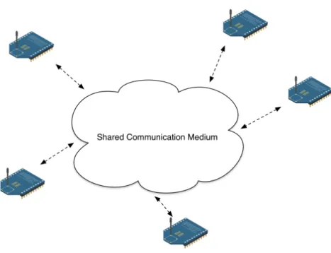
3.1 Medium Sharing Between Nodes . . . 39
3.2 Classification of Existing MAC Protocols . . . 44
3.3 Fixed Assignment Multiple Access [121] . . . 45
3.4 Contention Process of CSMA/CA . . . 51
3.5 Contention process of Pure ALOHA . . . 52
3.6 Throughput performance of Pure ALOHA . . . 52
3.7 Contention process of Slotted ALOHA . . . 53
3.8 Throughput performance of Slotted ALOHA . . . 54
3.9 S-MAC wake-up and sleep modes of operation . . . 55
3.11 Contention Process of T-MAC . . . 57
3.12 Superframe Structure of IEEE 802.15.4 . . . 60
3.13 The Workflow of ALOHA-Q . . . 63
4.1 The Network Domain . . . 70
4.2 The Node Domain . . . 71
4.3 The Process Domain . . . 72
4.4 The Radio Transceiver Pipeline . . . 73
5.1 The Time Slot Structure . . . 81
5.2 Typical Single-Hop Based WSN . . . 83
5.3 Topology of the Simulated Single-hop Network . . . 84
5.4 Comparison of Throughput Performance . . . 85
5.5 Comparison of Average End to End Delay Performance . . . 86
5.6 Comparison of Average System Convergence Time . . . 87
5.7 General Workflow of DFA . . . 91
5.8 Frame Size Adjusting Process for 10 Nodes . . . 92
5.9 The Changing Trend of Highest Q value for Steady and Unsteady Nodes 93 5.10 Proactive Jamming Strategy . . . 94
5.11 Frame Size Adaptation Process for Individual Nodes . . . 97
5.11 Frame Size Adaptation Process for Individual Nodes . . . 98
5.12 Real Time Number of Steady Nodes . . . 99
5.13 Real Time Running Throughput . . . 100
6.1 Example of Linear Chain Network . . . 104
6.2 Randomly Deployed Linear Chain Multi-hop Network . . . 105
6.3 Example of Cross Chain Multi-hop Network . . . 106
6.4 Linear Chain Network . . . 107
6.5 Comparison of Throughput Performance . . . 110
6.6 Comparison of Throughput Performance . . . 112
6.8 Hidden Node Problem . . . 114
6.9 The Workflow of Slot Swapping Technique . . . 118
6.10 The Comparison of Average End-to-end Throughput Performance with Slot Swapping . . . 120
6.11 The CDF of End-to-end Throughput Performance with Slot Swapping 120 6.12 The Workflow of Frame Size Evaluating Process . . . 122
6.13 Linear Chain Network . . . 125
6.14 Frame Size Adaptation Process for Individual Nodes . . . 126
6.15 Comparison of Real-time Offered Traffic and Throughput for Route A 127 6.16 Comparison of Real-time Offered Traffic and Throughput for Route B 127 6.17 Example of Cross Chain Network . . . 128
6.18 Subframe Structure . . . 129
6.19 Cross Chain Network . . . 133
6.20 Subframe Adaptation Process . . . 134
6.21 Real-time Probability of Successful Transmission . . . 135
List of Tables
2.1 Current consumption for IRIS and MICA-2 motes . . . 34
5.1 Simulation Parameters I . . . 80
6.1 Simulation Parameters II . . . 111
6.2 Simulation Parameters III . . . 124
Acknowledgements
I would like to dedicate this thesis to my parents for their love and support in my Ph.D. life. They have always encouraged me towards excellence.
My deepest gratitude is to Dr. Paul Daniel Mitchell for his patience, encouragement and persistent help throughout the past four years. As my first supervisor, Paul always give me immense knowledge and unique insights about my research work. Without his guidance, this thesis would not have been possible. I would also like to gratefully acknowledge the valuable help from my thesis advisor Dr. David Grace and my second supervisor Mr. Tim Clarke. They always give me inspiration and guidance, which is really beneficial to my research progress.
In addition, I want to extend my appreciation to my friends, colleagues and experts from the communications and signal processing group, their support is very important to my research as well. All in all, the merits of this thesis are due to the good efforts of contributors mentioned above, I wish to express my sincere gratitude to them.
Declaration
To the best knowledge of the author, all work in this thesis claimed as original is so. Any research not original is clearly specified. References and acknowledgements to other researchers have been given as appropriate. In addition, I certify that this thesis was never submitted in my name, for any other degree or diploma in any university or other tertiary institution.
Chapter 1
Introduction
Contents
1.1 Research Background . . . 1
1.2 Overview of Medium Access Control Layer . . . 4
1.3 Overview of Reinforcement Learning Technique . . . 5
1.3.1 Q-learning . . . 8
1.4 The Scope of Thesis . . . 11
1.5 Thesis Outline . . . 13
1.1
Research Background
This thesis focuses on the techniques and challenges concerning the design of intelli-gent Medium Access Control Protocols for WSNs. The concept of WSNs originated in the 1950s. The earliest application was the Sound Surveillance System (SOSUS), designed by the United States Military for the purpose of detecting and tracking sub-marines [1]. This system contains a large number of acoustic sensors deployed in the Atlantic and Pacific oceans for gathering sound signals. Since then, sensing and wireless communication technologies have been constantly and gradually developed
throughout the 1960s and 1970s. In the early 1980s, the Defence Advanced Research Projects Agency (DARPA) initiated the modern WSN programme called Distributed Sensor Networks (DSN) [4]. The creation of DSN led researchers to realise the po-tential benefits of WSNs in consumer markets. From the mid of 1990s to the present, WSN technology became an important focus in academia and civilian scientific re-search. As a multidisciplinary technology, WSNs merge a wide range of techniques of wireless communication and networking, distributed sensing, signal processing and pervasive computing. A wireless sensor network is a system consisting of densely dis-tributed sensor nodes that gives people the capability to observe and react to events and phenomena within a specific sensing area [2]. Currently, WSNs play a key role in real-time information monitoring and collection due to their flexibility and efficiency. To some extent, WSNs represent the unique means of real-time remote information sensing and collecting.
WSNs have been developed for decades, but the market demands were mainly driven by the military and heavy industry. After entering the 21st century, corresponding research gained increasing attention due to breakthroughs in multiple key areas. As the standardisation of CMOS processing technologies for most semiconductor compo-nents begun from early 2000s. Network designer can use simplified hardware solutions such as wireless Micro-controllers (MCUs) that usually consist of a general-purpose MCU and an RF transceiver in a single chip. Therefore, the cost of high node count WSN applications finally reaches an affordable level. Besides, the development of battery and energy harvesting technologies enable longer operation of sensor nodes. Moreover, System-on-Chip (SoC) [3] integration technology has achieved unprece-dented development during the past decade. Sensing units, processing units, memory and antennas can be integrated at a cubic millimetre sized scale. Owing to those tech-nological advances, the production of small-sized, low-cost and multifunctional wire-less sensor nodes becomes technically and economically feasible. The current trend of WSNs turns towards long term distributed sensing and intelligent self-maintenance [94]. Sensor nodes can be eventually deployed on any physical object and in any
ge-ographic area, perform various applications in diverse environments, including soil, natural habitats, oceans, volcanoes and the human body. In the near future, WSNs are expected to be integrated into many life-changing technologies such as the Internet of Things and Smart Cities [95]. Across a wide range of applications, sensor networks can help us to understand and manage an increasingly interconnected physical world. Energy efficiency of wireless sensor nodes is usually treated as the paramount priority while designing a WSN [6]. It determines the operating period of WSNs due to the battery-driven nature of typical wireless sensor nodes. How to minimise the power consumption of nodes, on the condition that the reliability of the data transmission is guaranteed, is an important research topic for WSNs. To eliminate power ineffi-ciencies, researchers have devoted substantial effort to extend the lifetime of sensor nodes from all aspects. Current studies about the energy consumption of sensor net-works suggest that the power consumption of nodes is strongly dependent on their radio modes which are directly controlled by the Medium Access Control (MAC) pro-tocols [13]. MAC propro-tocols aims to regulate radio activities of nodes and coordinate channel sharing in order to avoid retransmissions, idle listening, overhearing and other energy waste activities. Consequently, the design of efficient MAC protocols plays a decisive role in ensuring system QoS and prolonging the operation time of sensor nodes. Compared to conventional wireless networks, the design of MAC protocols for WSNs needs to overcome some unique challenges about hardware constraints, power consumption, channel bandwidth, topology management, etc. The demand for higher channel utilisation and reduction in the coordination overheads intensifies the need for an intelligent channel sharing policy. The network uncertainty associated with en-vironmental changes creates the demand for node self-organisation. In addition, to improve the reliability and efficiency of protocol implementation, a simpler operation mechanism is desired.
1.2
Overview of Medium Access Control Layer
WSNs rely on a group of protocols that are running concurrently to fulfil required ap-plications. Those protocols are need to be properly managed to ensure the operation of individual sensor nodes and increase the overall efficiency of the network. Therefore, a protocol stack architecture is required to standardise and abstract the internal functions of sensor nodes. The protocol stack of WSNs is similar to Open Systems Interconnec-tion (OSI) network model proposed by InternaInterconnec-tional OrganizaInterconnec-tion for StandardizaInterconnec-tion (ISO). OSI model divides the communication functions of an open system into seven logical layers including physical layer, data link layer, network layer, transport layer, session layer, presentation layer and application layer [12]. Each layer deals with a particular problem. Compared to standard OSI model, the WSNs have a relative sim-plified protocol stack (see Fig. 1.1) due to their unique characteristics [13].
Amongst the layers demonstrated in Fig. 1.1, this thesis puts emphasis on the Media Access Control (MAC) layer which plays significant role in channel utilisation, system Quality of Service (QoS) and the lifetime of sensor nodes. The Media Access Control Layer is one of the two sublayers that form the Data Link Layer (DLL). The MAC sublayer is located above the physical layer and it is responsible for the following basic functions.
• Frame encapsulation and disassembling.
• Addressing of destination stations.
• Conveyance of source-station addressing information.
• Protection against errors, generally by means of generating and .checking frame check sequences.
• coordination of access to the physical communication medium.
The prime focus of MAC layer is the channel access control mechanisms which are also known as MAC protocols [15]. A MAC protocol is composed of a set of rules
Figure 1.1: Protocol Stack of WSNs
allow multiple stations connected to the same physical medium to share it. Compared to wired networks such as ethernet. The data transmission of wireless networks can be easily disturbed due to channel noise, long range signal fading and environmental issues, so that the design of an efficient MAC protocol is vitally important for WSNs to successfully carry out their required operations.
1.3
Overview of Reinforcement Learning Technique
To improve the intelligence of sensor nodes for access channel, this research exploits reinforcement learning techniques, which are specific learning algorithms in the ma-chine learning family. Reinforcement learning is expected to enable sensor nodes to
form an optimal scheduling policy without consuming any significant control over-heads [53]. In a general sense, machine learning is a subfield of artificial intelligence concerned with techniques that intelligent systems (i.e. computers, robots, sensor nodes.) simulating the learning behaviour of humans with the purpose of imbibing knowledge and skills from the external environment [89]. Machine learning allows learners to gain experience by doing tasks and then improve their performance on the same task or similar tasks in the domain. A learner is composed of a learning module, database and action module. These components help a learner capture useful informa-tion from the environment according to supervised or unsupervised approaches. The core idea of reinforcement learning is simple: when a learning process starts, the action module firstly executes random interaction between the learner and the environment [88]. The information from the environment will then be converted into the valuable experience by the learning module. These experience are always stored in the database module. From the next interaction, an improved action will be performed by analysing the database.
Figure 1.2: Reinforcement Learning Process
As an important machine learning category, reinforcement learning has been widely applied in many areas including intelligent robots, financial forecasting and analysis,
etc [87]. It can be considered as a computational algorithm for transforming real-world situations into actions. As Fig. 1.2 shows, a typical reinforcement learning process can be divided into two sub-processes: learning process and exploitation process. During the learning process, a learner attempts to obtain an optimal policy for achieving its goal. Specifically, a learner performs a random action and environment will respond a feedback to the learner at the beginning of the learning process. Subsequently, the learner transforms the received feedback into reward or punishment value and then evaluate which is the optimal action based on a specific reward function. Any action performed by a learner also affects subsequent actions and rewards. In this manner, a learner continuously reinforces its actions by receiving feedback from the environment. After a period of time, the learner is expected to find an optimal action policy which always leads to maximum reward, it then enters an exploitation status where the learner does not need to gather more experience but makes best action according to current policy.
Compared to supervised learning algorithms, reinforcement learning does not assume that labelled or explicit patterns or examples are given to the learner for training. More-over, reinforcement learning differs from unsupervised learning in that it introduces the error or reward signal to evaluate a potential solution. In reinforcement learning, a learner is not told directly what to do or which action to take. Instead, reinforcement learning eliminates examples and requires that the learners form and evaluate concepts based on action/reward functions. There are two important features of reinforcement learning: trial-and-error search and delayed reinforcement [88]. The learners are able to learn an optimal policy for accomplishing goals by trial, error and feedback. In order to optimise reward possibilities, the learner should not just do what it already knows but must explore further options. Generally, exploration must be made multiple times to gain reliable estimates of rewards. The learner that explores more has a higher prob-ability to make the best selection in future, but learners who rarely explore or never explore can struggle to learn useful knowledge from the environment.
actions A. In the Markov Decision Process (MDP), during every discrete time t, a learner will observe its current statestthen take an optimal actionat. The environment will respond toat with a reward rt =r(st,at), and generate a subsequent statest+1= σ(st,at). In MDP,σ(st,at)andrt=r(st,at)just relate to the current state and action
pair of a learner rather than a historic state and action pair. The main task of the learner is to maximise the control policyπ:S→Ato accomplish its task. The control policy defines the learner’s choices and methods of action at any given time, it helps the learner take the most appropriate actionat based on the current statest. In order to make precise decisions, a learner keeps an accumulated valueVπ(st) =∑i∞=0σirt+i
by obey the control policy π. The actionat brings highestVπ(st), so a learner has to estimate and then re-estimate from the successes and failures over time. In fact, the most important aspect of reinforcement learning is to create the accumulated value for efficiently determining actions.
1.3.1
Q-learning
Q-learning is a model-free reinforcement learning technique. It enables learner to learn an optimal policy from local experience without require established state to action (S→A) policies [88]. Therefore, a learner can explore an optimal action policy in unknown environments. In Q-learning, the experience of a learner is represented by a Q-value (Q[S,A]), which is a function of state-action pairs to learned values. By executing different actions, the learner can move from state to state. Performing a particular action aoffers the learner a reward r. The main objective of the learner is to maximum its total reward. To achieve this, a learner maintains a table of Q[S,A], whereSis the tuple of states andAis the tuple of actions.Q[S,A]represents a learner’s current estimate of Q-value. During the learning process, the learner always takes the action which is expected to result in the highestQ[S,A].
The procedure of Q-learning algorithm can be summarised as follows:
• Observe the current state,si
• Choose an actionaifor that state based on currentQs,a.
• Execute the actionai.
• Receive immediate rewardri.
• Update the table entryQsi,aias follows:
Qsi+1,ai+1 = (1−α)Qsi,ai+α(r+maxQsi,ai). (1.1) Whereα is called learning rate, and controls the extent to which the newly acquired experience will override the past experience. Whenα =0, the learner will not learn anything while α =1 will make the learner only learn the most recent experience. When solving a stochastic problem, a small constant learning rate (such as 0.1) is used so the learner can find the optimal policy quickly.γ is a discount factor, which decides the importance of expected rewards. When γ =0, the learner only considers instant rewards while γ approaching 1 will make the learner pursue long-term high rewards. The introduction of learning rate and discount factor allows learner to decide its future actions according to instant rewards or accumulate rewards.
The Following example illustrates how Q-learning can be used to solve a practical problem. Consider there are 5 rooms (A, B, C, D and E) in a building. Rooms are interconnected by doors as shown in Fig. 1.3. We put a learner in room C and ask it to learn how to get out of this building in an optimal way. In other words, the learner has to reach F from its current location. Fig. 1.4 shows a simplified graph (of Fig. 1.3). Individual arrows represent mono-directional paths from one room to another, and each arrow is associated with a reward value. The paths that directly connect to F have an instant reward 100, the rest of paths which do not directly lead to F have zero rewards. In the context of Q-learning, each room can be considered as astateand the learner’s movement refers toaction.
Figure 1.3: Example of Q-learning
Figure 1.4: Simplified Environment
When the learner is in the initial state C, it can only go the state D since C is directly connected to D. From state D, the learner has three possible actions: either go to state B or E or back to state C. Once the learner reaches state E, the possible actions are go to state A, F or D. Moreover, if the learner is in state B, it can either go to state F or state D. From state A, the learner can only go back to state E. The state diagram and instant reward values can be represented by following matrixQ:
Each row of matrixQrepresents a unique state, and each columns refers to a possible action leading to the next state. The matrixQis initialised to zero prior to the beginning
Q= A B C D E F A − − − − 0 − B − − − 0 − 100 C − − − 0 − − D − 0 0 − 0 − E 0 − − 0 − 100 F − 0 − − 0 100
of learning process. When the learner stays in a certain state, it updatesQs,aby
assign-ing specific reward value fromQbased on (1.1). For example, let assume the discount value is 0.8 and learning rate is 0.1. Therefore,QSD,SB=0+0.1(0.8+max(0,100))=10.08. Accordingly, the Q-value tables can be continuously updated when the learner gains more and more experience through state-action pairs. MatrixQwill eventually reach a convergence point (where the leaner keeps updating its Q-value function but the value ofQs,aremains the same) such as:
Q= A B C D E F A − − − − 90 − B − − − 74 − 100 C − − − 74 − − D − 90 71 − 90 − E 74 − − 74 − 100 F − 90 − − 90 100
Subsequently, an optimal path to F is obtained by the leaner, which is C→D→B→F.
1.4
The Scope of Thesis
This thesis presents the design and evaluation of intelligent MAC protocols for WSNs with particular focus on addressing the challenges faced by their practical operation.
The ultimate goal is to apply the proposed MAC protocols into broadly dispersed high-node-count applications such as target tracking and event monitoring applications. This thesis starts out by introducing basic knowledge of WSNs and MAC protocols so as to profoundly understand the various techniques and challenges among MAC design. Existing MAC schemes struggle to achieve a high level of channel utilisation with a relatively simple operating mechanism. CSMA/CA-based schemes have been shown to solve the hidden node problem ineffectively and consume significant control overheads [14]. Time-division schemes often require strict time synchronisation and continuous centralised control that may increase the cost of system maintenance [15]. To successfully complete required missions, nodes are supposed to self-organise their operations to deal with underlying challenges resulting from environmental changes. Recently, a novel machine learning based MAC scheme called ALOHA-Q has been proposed [66]. ALOHA-Q utilises a frame-slotted structure and a Q-learning based slot-selection strategy. It combines the general merits of free and contention-based protocols but eliminates their shortcomings. In ALOHA-Q, a node can manip-ulate its transmission history in order to form an unique scheduling strategy. The transmission behaviour of nodes starts in a contention-based manner but eventually ends up with contention-free based performance level. Nodes need to expand a cer-tain amount of overhead at the beginning of network operation but they can enjoy the hugely improved throughput performance during the remaining lifetime. ALOHA-Q was originally applied to a single-hop network model and its performance has been examined in both software and hardware platforms. The simulation results from [66] suggested that the throughput of ALOHA-Q protocol is as good as TDMA under sat-urated traffic conditions, and the average convergence time of the whole system is predictable if the optimal number of slots per frame is selected. The study in [67] has applied the ALOHA-Q into real sensor test-beds, and corresponding practical results also showed the power of ALOHA-Q on improving throughput and delay performance. However, the implementation of ALOHA-Q relies on a known number of active nodes and relatively stable network environment. With a rapid increase of network scale
and node populations, a multi-hop based data transmission strategy gains popularity in mainstream WSN applications. This trend brings extra challenges to MAC proto-col design, such like the uncertainty of network size, unpredictable node interference range, dynamic network topologies, unstable traffic loads, etc. In this thesis, several novel schemes are presented in order to improve the functionalities of ALOHA-Q. The contribution of this research includes, but is not limited to:
• Designing a distributed and intelligent frame size adaptation scheme for max-imising the performance of ALOHA-Q under single-hop and multi-hop condi-tions.
• Developing a slot swapping scheme for helping ALOHA-Q to overcome hidden nodes problem under multi-hop conditions.
• Introducing a sub-frame adaptation scheme which allows sensor nodes to assign unique scheduling policies to individual incoming traffic flows and proposal of a set of self-organisation functions to sensor nodes for the purpose of achieve optimal performance level in event-driven sensor networks.
1.5
Thesis Outline
The rest of thesis is divided into seven chapters and the structure is presented in Fig. 1.5 Chapter II begins with a brief introductory survey about the evolution of WSNs. The classification and the layered models of WSNs are presented, followed by an investi-gation into basic wireless sensor node technologies. Several representative WSN ap-plications are introduced. Moreover, design challenges and technical hurdles of WSNs are summarised.
Chapter III places special focus on the Medium Access Control protocols of WSNs. This chapter begins with an exposition about the fundamental aspects of MAC proto-cols including performance trade-offs, energy efficiency design and MAC taxonomy.
Figure 1.5: Thesis Outline
Several representative MAC protocols are introduced, include the discussion of their pros and cons. Subsequently, a machine learning MAC scheme named as ALOHA-Q is introduced.
Chapter IV covers the discussion of the simulation techniques and the validation meth-ods. Software based simulation techniques and theoretical modelling methodologies are presented, followed by an introduction of the performance measures used to evalu-ate the proposed protocols.
Chapter V investigates the relationship between frame size selection and throughput performance of ALOHA-Q under single-hop conditions. A frame size adaptation scheme of ALOHA-Q for single-hop networks is proposed and analysed for the pur-pose of dealing with the uncertainty of node population.
Chapter VI investigates the challenges when implementing ALOHA-Q in multi-hop networks. The impact of the hidden node problem on throughput performance of ALOHA-Q in linear chain networks is analysed and simulated. A slot-swapping
tech-nique is proposed to resolve potential traffic congestion caused by the effect of hidden nodes. Besides, a frame size adaptation scheme specifically designed for linear chain networks is also introduced and analysed. The later sections of this chapter intro-duce a subframe adaptation scheme, which help sensor nodes to achieve collision-free scheduling in cross chain networks. Plentiful simulation results are illustrated to high-light unique features and evaluate the overall performance of proposed schemes and techniques.
Chapter VII provides potential further research to extend this thesis. The frame size adaptation schemes introduced in this thesis can be enhanced to achieve better chan-nel utilisation for event-centric applications. Moreover, the introduction of intelligent duty cycle mechanism and Lifelong Machine Learning (LML) algorithm can further improve the adaptivity and energy efficiency of proposed MAC protocols.
Chapter VIII concludes the work in this thesis. The unique contributions are high-lighted followed by corresponding publications developed as a result of the work un-dertaken.
Chapter 2
Fundamentals of Wireless Sensor
Networks
Contents
2.1 A Brief History of Wireless Sensor Networks . . . 17
2.2 System Classification . . . 18
2.3 Sensor Node Technology . . . 20
2.3.1 Basic Functionalities . . . 20
2.3.2 Node Architecture . . . 23
2.4 Communication Protocol Stack . . . 26
2.5 Current Applications . . . 28
2.5.1 Environmental Application: Habitat Monitoring . . . 28
2.5.2 Military Application: Smart Dust . . . 30
2.5.3 Health Application: Wearable Medical Sensors . . . 31
2.5.4 Summary . . . 32
2.6 Design Challenges . . . 33
2.1
A Brief History of Wireless Sensor Networks
A wireless sensor network (WSN) is an infrastructure comprising a group of spatially dispersed sensor nodes, which are responsible for measuring parameters from a spe-cific geographic area [13]. WSNs have become an active research field and intensively studied over the past few decades. During the early stage, related applications were mainly designed to fulfil either military or scientific research purposes, and the cor-responding research were limited in universities and institutes. In the early 1980s, the development of WSNs has gained the major impetus from the Distributed Sensor Network (DSN) program of the Defence Advanced Research Agency (DARPA). DSN initialised numerous novel techniques relate to distributed sensing, signal processing and wireless networking. It applied the newly established Transmission Control Proto-col/Internet Protocol (TCP/IP) protocols and ARPnet’s (the predecessor of the internet) technologies to the context of sensor networks. Based on the outcomes of the DSN pro-gram, some well-known corporations like Intel, Boeing, Motorola and Siemens and their academic partners such as Carnegie Mellon University and the Massachusetts Institute of Technology have greatly promoted the development of the sensor hard-ware, the application softhard-ware, and the network protocols of WSNs [4]. As a conse-quence, WSNs have been applied to many fields for various purposes (i.e., environment monitoring, traffic management, healthcare, industrial production). These applications promise tremendous societal benefits, from disaster prevention to productivity increas-ing. From the late 1990s, advances in semiconductor, distributed computing, wireless communication, and energy storage result in a new generation of WSNs. Today’s state-of-the-art WSNs employ inexpensive compact sensor nodes that can complete required tasks in a collaborative way and self-organise their operations [10]. Com-pared to traditional WSNs, the cost of deployment and the complexity of maintenance are significantly reduced. The evolved WSNs support a diverse range of connectivity technologies and network standards so that sensed information can easily be uploaded to the internet through wireless access points (as Fig. 2.1 shows). This offers a huge improvement in the flexibility of information access. WSNs are finding their way into
countless applications in our homes, offices, factories, and beyond, provide an unprece-dented way to help people to capture information about various real-world phenomena and convert these information into a form that can be further processed and shared.
Figure 2.1: Modern Wireless Sensor Network Arrangement
2.2
System Classification
There has been extensive science and engineering progress on WSNs over the recent decade. The high-speed development of WSNs enables a wide range of applications for information sensing and controlling. Conventional WSN applications are distinct from each other in operating scenarios. From an applications perspective, WSN systems can be classified into the following two categories [4]:
• Category 1 Wireless Sensor Networks (C1WSNs): they represent the mesh-based WSN system with multi-hop wireless connectivity between source nodes and forwarding nodes (see Fig. 2.2). Source nodes refer to the sensor nodes in the usual sense, which can capture, transmit and receive information. In practical scenarios, the distance between a source node and the back-end data sink may be too far to establish a direct radio link. Therefore, the messages generated from
Figure 2.2: Category 1 WSNs
source nodes need to be relayed by intermediate devices called forwarding nodes that might be multiple link hops away from a source node. Forwarding nodes are interconnected via wireless links. Each of them acts as a wireless router that bridges the source nodes and the data sink. They can process and/or compress the messages from neighbouring source nodes, and send these messages to the data sink via an optimal route by using a dynamic routing technique.
• Category 2 Wireless Sensor Networks (C2WSNs): they are networks in which source nodes are one link hop away from each forwarding node (see Fig. 2.3). The major characteristics include: there is no direct link between any two source nodes; Forwarding nodes support static routing technique instead of dynamic routing; Forwarding nodes cannot process and/or compress the sensed message on the behalf of source nodes.
The two categories of WSNs have different scopes. C1WSNs focus the large-scale highly distributed WSN systems. These systems usually cover a broad sensing area, and individual sensors are assumed to self-operate over a relatively long period. Corre-sponding applications include habitat monitoring and battlefield surveillance. C2WSNs
Figure 2.3: Category 2 WSNs
tend to handle the short-range single-hop systems with low traffic loads. Related appli-cations include the Radio Frequency Identification (RFID), Indoor Intrusion Detection, and Wearable Human Health Monitoring.
2.3
Sensor Node Technology
2.3.1
Basic Functionalities
Wireless sensor nodes (also referred to motes) are the fundamental element of a WSN. They provide the functionalities of sensing, processing and communication by exe-cuting built-in communication protocols, data-processing algorithms and application programs. The design and implementation of sensor nodes determine the quality of information which can be accessed by the network. As technology-intensive research, the development of wireless sensor nodes were stymied by many technical issues dur-ing the early stages. Since the early 1990s, advances in Micro Electro Mechanical Systems (MEMs), SoC, Wireless Communications and Low Power Consumption
Em-bedded technologies has enabled the great development of wireless sensor networks (WSNs). It has become technically and economically possible to manufacture power-ful small-sized (According to the needs of the application, the size of a sensor node may vary from the size of a shoe box to a microscopically small particle) and low-cost wireless sensor nodes such as the example shown as Fig. 2.4.
Figure 2.4: Typical Sensor Mote [117]
From a functional perspective, wireless sensor nodes combine physical sensing of pa-rameters with computation and networking capabilities. The main responsibility of a sensor node is cover a geographic area in order to monitor certain parameters [13]. These parameters include but not limited to, mechanical, chemical, thermal, electri-cal, chromatographic, magnetic, biologielectri-cal, optielectri-cal, ultrasonic information. Further-more, sensor nodes have wireless communication capabilities and some logic for data sensing, signal processing and transmission handling. The basic functionalities of a wireless sensor node mainly depend on a specific application, but the following re-quirements are typical.
• Determine the value of a parameter at a given locations: for example, in a environment-oriented WSN, one may need to capture the temperature of the
crater of a volcano, sense the atmospheric pressure of aircrafts, or obtain the value of humidity in a room.
• Detect the occurrence of interesting events and estimate the parameters of the events: for instance, in a traffic-oriented sensor network, one would like to detect a vehicle is moving through an intersection and estimate the speed and direction of the vehicle.
• Classify an object that has been detected: for example, whether a fire disas-ter occurs in sensing areas by comparing the current values of temperature and smoke particle density with the threshold values.
• Track an object: for example, in a military sensor network, track an enemy vehicle as it moves through the battlefield a covered by wireless sensor nodes.
Typical parameters that can be measured by sensor nodes include:
• Physical measurement: examples include speed and displacement (accelerome-ters measure acceleration); radiation levels (Ionisation detectors); acoustic wave’s intensity (resonators) and location (Global Positioning System (GPS)).
• Chemical and biological measurement: examples include the air composition (infrared gas sensors); body acidity or alkalinity (PH sensors) and elements of drugs (electrochemical sensors).
Some of the design requirements that sensor nodes need take into account include the following:
• For military and security applications, sensor nodes need to support rapid de-ployment which must be supportable in an ad-hoc manner.
• Sensor nodes may be prone to failure, unattended, untethered, self-powered low-duty-cycle.
• The topology that the sensor nodes need to maintain may change very frequently. the cost of supporting high-capacity and long-range communications may be expensive.
• Sensor nodes may not have global addresses due to the potentially large number of nodes and overhead needed to support such global addresses.
• Sensor nodes usually require in-network processing, even while data are being routed. Typical processing jobs involve signal processing, data aggregation, data fusion, and data analysis.
• Sensor nodes may be deployed in a dense manner. The level of node local inter-ference is not predictable.
2.3.2
Node Architecture
Wireless sensor nodes come in a variety of hardware components, and these compo-nents can be categorised into four subsystems: sensing, processing, communication and power storage [8]. Fig. 2.5 shows the architecture of a typical wireless sensor node. The power subsystem and its relationship with the other subsystems are not shown here. The sensing subsystem is the interface between the virtual data and ical world. It is responsible for the measurement and quantification of interested phys-ical attributes. A sensing subsystem consists of single or multiple sensing units and/or analog to digital signal converters. It is through these components that the target infor-mation are converted into meaningful discrete digital signals. The processing subsys-tem can be thought of as a data hub that connects to the rest of subsyssubsys-tems and addi-tional peripherals. This subsystem is used to handle processing and management tasks including data processing and manipulation, short-term data storage, digital modula-tion, self-organisation and communication control. To fulfil these tasks, the processing subsystem includes one of components from a micro-controller, Digital Signal Pro-cessor (DSP), Application-Specific Integrated Circuit (ASIC), or Field-Programmable Gate Array (FPGA) according to its needs [4]. The selection and implementation of
each component of the processing subsystem are vital to the performance, cost, as well as the energy consumption of a sensor node. The communication subsystem is mainly composed of a radio transceiver. It is capable of establishing radio connectiv-ity between sensor nodes and to transmit the encrypted data packets output from the processing subsystem. As a energy intensive subsystem, the operation of the com-munication subsystem is critical to the energy-efficiency of a sensor node as well as the overall efficiency of a network [8]. Finally, the power subsystem which usually contains a built-in battery or energy harvesting component provides sustained energy to all the other subsystems. Clearly, the architecture of sensor nodes varies with cost, application and operating environment. However, typical sensor nodes are comprised of some necessary components which are introduced as follows
Figure 2.5: Architecture of Typical Wireless Sensor Nodes
• Sensing unitsare devices that produce a measurable response to a change in a physical condition. That converts a form of energy quantity (usually voltage) into analog signals. Typical sensing units can be classified as passive or active units. Passive sensing units tend to be low-energy devices as they just rely on environmental changes. Corresponding examples include the measurement of acoustic waves, humidity, temperature, and vibration. On the contrary, active sensing units transmit probing signals (e.g., microwaves, light, sound, infrared) to a target and then capture the interesting information by detecting the changes
in the energy of the transmitted signals. Related examples include ultrasonic measuring and infrared measuring.
• Micro-controllershave been used widely by most embedded systems including home appliances, vending machines, elevators, etc. It is a miniaturised pro-grammable computer that performs most functions of a typical personal com-puter. A micro-controller contains the following units: a Central Processing Unit (CPU) a Random Access Memory (RAM) unit, programmable input/output in-terfaces and a clock generator. Amongst these units, the CPU is the core element of a micro-controller. It is responsible for handling the locally collected data or the received data from other sensor nodes, and supervise different components of a sensor node. The most prominent advantages of micro-controllers is their programming flexibility, which enables developers to reduce the cost and time when trying to adapt new algorithms and applications to a given sensor node. Sometimes, micro-controllers can be replaced by DSP or FPGA if the applica-tions required intensive computation or high speed data acquisition [13].
• Radio transceiver is the most necessary component of wireless sensor nodes. It is a single component but comprises both a transmitter and a receiver that are used to exchange information with other sensor nodes.Currently, frequen-cies used for wireless sensor systems include 315 MHz, 433 MHz, 868 MHz (Europe), 915 MHz (North America), and the 2.45-GHz Industrial-Scientific-Medical (ISM) band. When a sensor node is turned on, the radio transceiver has four operational states: transmitting, receiving, idle, and sleep [3]. A built-in coprocessor controls built-in which state the radio transceiver stays automatically. Compared to other onboard components, radio transceivers consume a signifi-cant amount of energy during operation time [45]. To reduce unnecessary en-ergy consumption, the transceiver is expected to stay in the idle or the sleep state when a node has no message to send. Therefore, the regulation of the data transmissions is the most important factor that affects the energy conservation of sensor nodes.
• Power supply takes charge of providing DC currents to each component of a sensor node. For a typical sensor node, the primary power supply is a built-in battery that could support the operation of sensor nodes rangbuilt-ing from a few days to several years. In addition to relying on its built-in batteries, an energy-harvesting device can also provide energy to sensor nodes from external sources including sunlight, water stream, wind and etc [97]. Currently, energy harvesting has become a key research topic due to its advantages of perpetual power supply, simple device and good portability. However, the operation of energy-harvesting devices has specific requirements regarding node operating environments and would increase the cost of sensor nodes.
Small, low-cost, robust and reliable wireless sensor nodes are needed to enable the wide-scale deployment of practical and economical WSNs, which are expected to be-come ubiquitous in the future for improving the quality of human life. The current trend of wireless sensor nodes includes several aspects: to enhance the sensitivity, the speed, and the robustness of data acquisition; to increase the functions to respond to more physical phenomenon; To improve the ability to complete tasks in complex and dynamic environments. to address these needs, advanced research in broadband wire-less communication, miniaturisation of embedded systems, pervasive computing and energy harvesting can be brought in the future stage [94].
2.4
Communication Protocol Stack
In addition to selecting superior sensor hardware, the most efficient approach to en-hancing the performance of a WSN is to design a set of flexible, robust and interoper-able networking protocols. A protocol refers to a rule that achieves a specific internal function of a node [96]. To characterise and standardise individual protocols of an open communication system, researchers introduced the concept of Open Systems In-terconnection (OSI) reference model. This model divides the system architecture into seven layers: physical layer; data link layer; network layer; transport layer; session
layer; presentation layer and application layer [12]. Each layer is composed of a group of protocols that deal with the same set of issues. The inspiration for the OSI reference model leads to a similar layered model for WSNs. Generally, Communication proto-cols of WSNs can be classified into five layers: physical layer, data link layer, network layer, transport layer and application layer [4]. The main descriptions of these layers are presented as follows.
• Physical layer: this layer consists of the basic transmission technologies of a node. It provides the means of generating raw bit streams and transmitting these streams over robust physical links between dispersed nodes. The functions per-formed by the physical layer protocols including medium and frequency selec-tion, signal detecselec-tion, carrier modulaselec-tion, data encrypselec-tion, etc.
• Data Link layer: this layer provides functional and procedural means to trans-mit data between nodes. The data link layer concerns some key issues like the utilisation of available radio resources and management of the transmission ac-tivity. As the interface between the physical layer and the upper layers, the data link layer is also responsible for detecting and correcting errors generated in the physical layer. The protocols of the data link layer are used to provide services related to medium access, error control, timing, and locality.
• Network layer: this layer is responsible for transmitting packets between a source node and a destination node while maintaining Quality of Service (QoS). The network layer protocols mainly focus on the services regard to routing, topology management, flow control, and congestion detection.
• Transport layer: the objective of the transport layer is to deliver data packets along a established transmission route. Transport layer protocols mainly con-cern the services related to data dissemination, caching, storage and congestion control. For WSNs, the design of transport layer protocols has unique focus. For example, how to achieve reliable transport in a WSN with dynamic topologies caused by node mobility, failure or power-down.
• Application layer: this layer directly connects to the application interface and mainly responsible for the execution of specific application services. As the highest layer, the application layer controls all the functions provided by lower layers. The protocols of the upper layer are mainly used to perform self-organisation tasks, including data processing and aggregation, time synchronisation, and clus-tering of nodes.
2.5
Current Applications
Through decades of development, envisaged sensor-network applications have been spread over the real world with commercial or military availability. The market scope of WSNs is expanding rapidly since the beginning of 21st century. Many academic institutes and companies have emerged as suppliers of the necessary hardware and software building blocks. Wireless sensor nodes have considerable deployment flexi-bility. They can be deployed in various sensing fields to detecting interesting events, to track moving targets, to support the operation of intelligent systems. The diversity of WSN applications can be remarkable, ranging from environment monitoring to human health care [10]. In this section, some representative applications are given to provide a better insight into the potential of WSNs.
2.5.1
Environmental Application: Habitat Monitoring
The evolution of wireless sensor networks has enabled new classes of applications that benefit the environmental monitoring domain. In recent decades, many research groups have proposed using WSNs for habitat monitoring. Traditional data loggers for habitat monitoring are typically large and expensive [11]. To obtain accurate results, probes need to be redeployed manually and constantly in different locations of the in-terest area. They also have to be connected to additional equipment for recording and analysing the collected raw data. Moreover, using probes often result in a ”shadow
effect”, a situation that occurs when an organism alters its behavioural patterns due to interference in their space or lifestyle. Instead, biologists argue for the small-sized de-vices that may be deployed on the surface, in burrows or trees. Since the interference is such a significant concern, the sensor must be inconspicuous. They should not disrupt the natural processes or behaviours of human or animal.
Figure 2.6: Habitat Monitoring Application [118]
WSNs represent a significant advance over the traditional methods of habitat moni-toring [9]. Small nodes can be deployed prior to the sensitive period (e.g., breeding season for animals, plant dormancy period). Besides, sensor nodes can be deployed in small areas where it would be unsafe or unwise to frequently reached by the human. A key difference between WSNs and traditional probes or data loggers is that WSNs per-mit real-time data access without repeated visits to habitats [11]. Moreover, deploying sensor networks is a more economical and efficient method for conducting long-term studies than traditional methods such as data loggers, since sensor nodes can be de-ployed and left easily in habitat areas. WSNs may organise themselves and store data that may be later retrieved and notify that the network needs servicing. With the help of WSNs, researchers could access more information that often limited by concerns
about disturbance or lack of easy access.
2.5.2
Military Application: Smart Dust
WSNs can be an integral part of military Command, Control, Communications, Com-puters, Intelligence, Surveillance, Reconnaissance, and Targeting (C4ISRT) systems. The clearest example is the Smart Dust project which was developed by UC Berke-ley in 1998 [7]. Researchers want to use most advanced technologies from MEMs and SOC with the purpose of producing ultra-small, ultra-light wireless sensors which could float in the air like dust (see Fig. 2.7). Similar to the typical application of WSNs, the smart dust is a complete sensor system. Each dust contains a sensing unit, micro-processor, transceiver and power supply, and all of these components are embedded into a cubic-millimetre package [18].
Figure 2.7: Smart Dust Application [119]
The US army believes that smart dust will play a crucial role in future battlefield mon-itoring systems, due to significant advantages in terms of reliability and fault-tolerance under harsh environmental conditions. The smart dust sensors can be deployed in a war zone by soldiers, vehicles or aircrafts. These sensors are usually randomly dis-tributed and work in a self-organised manner. The performance of the whole system would not be severely affected even if the malfunction occurs in some nodes. If one node goes down another will immediately pick up its task. Commonly, smart dust sen-sors can be classified as source nodes, sink nodes and target nodes. The source nodes
can collect real-time data of interest (i.e. position of enemies) and transmit perceived information to sink nodes through multi-hop communication routes. The sink nodes take charge of the analysis, processing and relaying of received data. Eventually, the data received by sink nodes will be further passed to data hubs out of the sensing area. Compared to traditional technologies, smart dust provides an invisible, low-cost and low-risk solution for gathering the useful data from a whole battlefield.
The prospect of the smart dust project is truly appealing. However, researchers still face a lot of technical issues that may restrict the development of smart dust for a relatively long period. With current technologies, it is difficult to integrate high-end electronic components into the expected cubic-millimetre package, so there will be a trade-off between performance and size. Moreover, power consumption is another challenge because the battery of the sensor is almost irreplaceable. Some of the re-searchers decide to investigate various low-power network protocols that are expected to help individual sensor nodes to reduce unnecessary power overheads.
2.5.3
Health Application: Wearable Medical Sensors
The use of WSNs in health care systems has yielded a tremendous effort in recent years [24]. Wearable health monitoring systems have gained great popularity during the past decade. These systems consist of multiple wearable medical sensors that can be easily placed in the human body to record their health status. The traditional health monitoring technologies are quite expensive and often feature unwieldy wires between the sensors and the control system. The activity and feeling of patients will be restricted and degraded by wires, so that affects the accuracy of the measured results. However, low weight and low-cost wearable medical sensors can provide a more convenient and affordable solution. Patients will benefit from continuous long-term, accurate, and real-time or near real-time monitoring. In addition, the wearable sensors could be connected with other telemedicine systems through the internet or some other wireless local networks [10]. Patients can make a medical enquiry at home, their physiological
measures such as body temperature, heart rate, blood pressure will be transmitted to a computer viewed by remote doctors who then make an instantaneous diagnose and return useful feedback to the patients. The advantages of wearable medical sensors could significantly reduce the time and cost for patients and hospitals.
Figure 2.8: Wearable Medical Sensor Networks [120]
2.5.4
Summary
In this section, a set of existing and possible WSN applications were introduced. WSNs have very broad application spectrum. Wherever people want to observe and react to events and phenomena in a particular environment, they can use WSNs. The environ-ment can be the physical world, a biological system, infrastructure or even IT frame-work. In terms of the market scope, WSNs are expected to see further expansion in the next decade. This expansion not only relates to science and engineering applications but also to upcoming new technologies from various emerging areas.
2.6
Design Challenges
WSNs offer powerful functionality of information sensing, data processing, and com-munication. They have brought about a plethora of applications and, in the meanwhile, bringing numerous technical challenges with respect to the unique traits of the sensor nodes and networks. The reliable and sustainable operation of WSNs is restricted with-out overcoming these challenges. The following section shows the major challenges that are shared among typical applications.
• Energy efficiency: energy efficiency is the paramount design consideration in WSNs. Wireless sensor nodes usually contain a limited built-in energy supply unit but are required to operate as long as possible in unpredictable environ-ments [4]. To replace or recharge sensor batteries is a difficult effort, especially for large scale networks. In fact, some design goals of sensor networks are to build nodes that are cheap enough to be discarded rather than reused or that are efficient enough to operate only on ambient power sources. In all cases, prolong-ing the lifetime of sensor nodes is a critical issue. Usprolong-ing low-power units and energy saving circuit design is a popular approach for reducing node power con-sumption [6]. The study [121] suggests that the power rating of a typical wireless sensor node which is supported by two 2.7V AAbatteries ranges from 10 mW to 1000 mW. Commonly, nodes consume a relatively small amount of energy when they sleep (processor off, sensor off, and radio off), but the energy con-sumption rises significantly when nodes switch from sleep state to active state (processor on, sensor on, radio on). The major energy consumption sources include communication, processing, status transient, sensor loggings and sens-ing [122]. These activities are controlled by different on-board units includsens-ing micro-controller (MCU), radio transceiver, and sensing unit. The following table presents the current consumption for two representative sensor node platforms: IRIS and MICA2.
con-Table 2.1: Current consumption for IRIS and MICA-2 motes Mote Type MCU Active MCU Sleep RF Tx RF Rx RF Sleep
IRIS 8 mA 8µA 17 mA 16 mA 0 mA
MICA2 8 mA <15µA 27 mA 10 mA <1µA
sists of a micro-controller, a radio transceiver, and a sensor board that can be in-terfaced to specific sensing units according to applications. It can be clearly seen that the radio transceiver of both motes has higher current consumption than their MCUs if they are not in sleep mode. SinceEnergy=Current∗Voltage∗Time, radio transceiver can be considered more energy intensive when compared to MCU. However, it does not mean that the radio transceiver always the largest power consumer. The actual energy consumption of a transceiver is also deter-mined by a number of factors including duty-cycle and data rate. Besides, some sophisticated sensing units such as infrared gas detectors may consume signif-icant amount of energy if compared with MCU and radio transceiver. When comes to MAC layer, the most efficient way of improve energy efficiency is to properly manage the activities of radio transceivers [8]. To achieve this, the communication of nodes need to be operated efficiently. In some cases, sensor nodes can be powered by energy-harvesting devices such as solar panels or wind turbines. However, the cost of system raises and the deployment environments will be restricted.
• Hardware performance: a sensor node may need to fit into a tight module. Due to the restriction in size, the performance of wireless sensor nodes is signif-icantly limited, especially in terms of processing capability (power consumption and cost of CPU), and the radio communication range (antenna size). In realistic scenarios, sensor nodes probably only have finite battery power but need to com-plete a large amount of tasks during the mission time or as long as possible [16]. Replacing the power sources of sensor nodes in a remote sensing field is usually not practicable. Sensor nodes also have to cooperate with adjacent nodes and
adapt themselves to the environmental changes, which requires additional data computation and processing. To conserve energy, typical sensor nodes integrates a low-power and single-channel transceiver. Therefore, the communications be-tween sensor nodes are more easily to be interrupted by noise signals.
• Traffic pattern: traffic pattern is an important consideration when designing WSNs. Modelling accurate traffic patterns brings great benefits to network op-timisation. For example, better MAC protocols or routing strategies can be de-signed if the traffic burden among individual sensor nodes is better investigated [125]. According to [126], existing WSN applications can be classified as pe-riodic or event-driven data generation. For pepe-riodic scenarios, the traffic arrival process follows either constant bit rate (CBR) where the bit rate [127] is always constant or Poisson distribution [128]. For event-driven scenarios, bursty traf-fic can arise from anywhere the sensing area when an event occurs. The burst phenomenon of the data generation can be simulated by ON/OFF model where the duration of ON/OFF periods follow the generalised Pareto distribution [129]. The WSNs simulated in this research are assumed to employ the Poisson based periodic traffic generation. The transmission data rate is set to 250kbps which fits the standard of IEEE 802.15.4 MAC layer. The ultimate goal is to achieve close-to-capacity throughput while fully eliminates packet collisions.
• Operating environment: sensor nodes may be deployed in harsh, hostile, or widely scattered environments. In such environments, nodes may die over time. The connectivity of network is easily affected by various environmental factors such as high electromagnetic interference, high humidity levels, vibrations, dirt and dust. Therefore, the reliability of a network may be threatened.
• Topology management: in some scenarios, sensor nodes are expected to be de-ployed in a random fashion so that the network topology is hardly to be predicted and managed [39]. For example, nodes could be dropped from a helicopter and the deployment location of each node is totally unknown. In more complex sit-uations, the network topology may ensue, as the nodes may malfunction due to
a lack of power or physical damage. To maintain reliable connections between nodes, an efficient mechanism is required to handle the changes of topology.
2.7
Summary
This chapter has introduced the basic concept of WSNs and supportive technologies. Typical WSNs are collections of miniaturised, inexpensive, self-operating computa-tional nodes. These nodes cooperate with to each other and organise themselves into a single-hop or multi-hop network. The unique characteristics of WSNs such as con-nectivity models of the network, system operating environments, and hardware and software constraints of nodes have brought great challenges to researchers. Under-standing these challenges is essential for the design and implementation of WSNs. Amongst all of these technical hurdles, the power consumption of nodes is the most important one since it directly affects the lifetime of entire network. In the following chapter, a technology called Medium Access Control (MAC) will be introduced, with detailed discussions of how MAC can be designed to improve the energy-efficiency of nodes.
Chapter 3
Medium Access Control Protocols
Contents
3.1 Fundamentals of MAC protocols . . . 38
3.1.1 Introduction . . . 38
3.1.2 MAC Design Trade-offs . . . 40
3.1.3 Energy Efficiency of MAC Design . . . 43
3.1.4 Taxonomy of MAC Protocols . . . 44
3.2 Examples of MAC protocols . . . 51
3.2.1 Pure ALOHA protocol . . . 51
3.2.2 Slotted ALOHA protocol . . . 53
3.2.3 Sensor-MAC protocol: S-MAC . . . 54
3.2.4 Timeout MAC protocol: T-MAC . . . 56
3.2.5 Zebra MAC protocol: Z-MAC . . . 58
3.2.6 IEEE 802.15.4 MAC layer . . . 58
3.3 ALOHA-Q . . . 62

![Figure 2.6: Habitat Monitoring Application [118]](https://thumb-us.123doks.com/thumbv2/123dok_us/1773181.2752300/41.892.236.722.325.693/figure-habitat-monitoring-application.webp)