Classification of Missing Youths Cases using Support Vector Machines

(1)

Classification of Missing Youths Cases using

Support Vector Machines

A Thesis Submitted to the

College of Graduate and Postdoctoral Studies

in Partial Fulfillment of the Requirements

for the degree of Master of Science

in the Department of Computer Science

University of Saskatchewan

Saskatoon

By

Maryam Orafaee Azghan

(2)

Permission to Use

In presenting this thesis in partial fulfilment of the requirements for a Postgraduate degree from the University of Saskatchewan, I agree that the Libraries of this University may make it freely available for inspection. I further agree that permission for copying of this thesis in any manner, in whole or in part, for scholarly purposes may be granted by the professor or professors who supervised my thesis work or, in their absence, by the Head of the Department or the Dean of the College in which my thesis work was done. It is understood that any copying or publication or use of this thesis or parts thereof for financial gain shall not be allowed without my written permission. It is also understood that due recognition shall be given to me and to the University of Saskatchewan in any scholarly use which may be made of any material in my thesis. Requests for permission to copy or to make other use of material in this thesis in whole or part should be addressed to:

Head of the Department of Computer Science 176 Thorvaldson Building 110 Science Place University of Saskatchewan Saskatoon, Saskatchewan S7N 5C9 Canada Or Dean

College of Graduate and Postdoctoral Studies University of Saskatchewan

116 Thorvaldson Building, 110 Science Place Saskatoon, Saskatchewan S7N 5C9

(3)

Abstract

A missing person is defined as a person who has been formally reported to the police as someone whose whereabouts are unknown. Many people go missing every year, and the vast majority of them are found or return home within one week. The purpose of this study is to provide the Saskatoon Police Service (SPS) with a set of predictive models for intervention and risk reduction applied to the missing youths (MY) database in a graphical user interface (GUI). The study is conducted on 434 missing persons cases with 91 features for each case. Two classification features are used to build the predictive models presented in this study. The first feature ismissing_again. This feature allows us to train a predictive model to assess the likelihood of a person to go missing again. The second feature is gang_involvement. This feature allows us to train a predictive model to assess the likelihood of a missing person will be involved in gang activity. The machine learning method Support Vector Machines (SVMs) is used to build models based on both classification variables and 91 items as input features for each MY case.

The SVM classifier obtained an accuracy of 89%, sensitivity of 84%, and specificity of 91% for the classification featuremissing_again. This classifier can be used by officers to consider when deciding whether or how to intervene in cases where youths are at a high risk to go missing again. The SVM classifier obtained an accuracy of 84%, sensitivity of 43%, and specificity of 90% for the classification featuregang_involvement. This classifier can be used by officers to determine whether a missing youth is likely to have gang affiliations. This knowledge could change how the case is approached and the safety measures the officers may take. The Ministry of Justice of Saskatchewan and the SPS also desire a graphical user interface for data analysis and reporting amenable for use by end users of the Missing Persons Project (MPP), e.g., police officers and data analysts.

(4)

Acknowledgements

I wish to thank my supervisor Prof. Raymond J. Spiteri for his fantastic guidance, support, and passion. The door to his office was always open whenever I ran into a trouble spot or had a question about my research or writing. I would like to give my thank you to my parents, and my husband, Navid, for providing me with continuous support and encouragement throughout my years of study, the process of researching and writing this thesis. This accomplishment would not have been possible without them. I would also like to thank the Saskatoon Police Services that provided me and the team I work with ethical access to the data worked with in this thesis.

(5)

List of Tables

3.1 Comparison of different kernel functions for the MY database . . . 15

3.2 A confusion matrix . . . 17

4.1 Basic information about the MY cases . . . 24

4.2 Basic statistics for age (years) . . . 24

4.3 Basic statistics for age grouped by gender (years) . . . 25

4.4 Basic statistics for time missing (days) . . . 25

4.5 Basic statistics for time missing grouped by gender (days) . . . 26

4.6 Basic statistics for repeat occurrences (number of times) . . . 26

4.7 Basic statistics for repeat occurrences grouped by gender (number of times) . . . 27

4.8 Basic statistics for time to the next event (days) . . . 28

4.9 Basic statistics for time to the next event grouped by gender (days) . . . 28

4.10 SVMs results for themissing_again classification feature (%) with10-fold cross-validation . . 29

4.11 SVM results for thegang_involvementclassification feature (%) with10-fold Cross-validation 32 4.12 SVM results in percent (%) . . . 34

(8)

List of Figures

3.1 How SVMs linearly classify data in a two-dimensional space . . . 10

3.2 Misclassified data using theξi variables . . . 12

3.3 Visualization of mapping data in a higher-dimensional space using a kernel method . . . 12

3.4 Visualization of SVM linear kernel . . . 13

3.5 Visualization of SVM polynomial kernel . . . 14

3.6 Visualization of SVM radial basis function kernel . . . 14

3.7 Visualization of SVM sigmoid kernel . . . 15

3.8 Logical diagram for the MY GUI . . . 22

3.9 Physical diagram of the MY GUI . . . 23

4.1 Histogram of age . . . 25

4.2 Histogram of time missing . . . 26

4.3 Histogram of repeat occurrences . . . 27

4.4 Histogram of time to next event. . . 28

4.5 Confusion matrix for the missing_againclassification feature . . . 30

4.6 Receiver Operating Characteristic curve for themissing_againclassification feature . . . 31

4.7 Confusion matrix for the gang_involvementclassification feature . . . 33

4.8 Receiver Operating Characteristic curve for thegang_involvementclassification feature . . . 33

A.1 Screenshot for “Login” page . . . 44

A.2 Screenshot for “Forgot Password?” page . . . 44

A.3 Screenshot for “Invalid Username/Password” page. . . 45

A.4 Screenshot for “Home” page . . . 46

A.5 Screenshot for specifying a date range using a calendar interface . . . 46

A.6 Screenshot for “Date Range” page. . . 47

A.7 Screenshot for “List” page . . . 47

A.8 Screenshot for “Heat Map” page. . . 48

A.9 Screenshot for Table Report . . . 49

A.10 Screenshot for Chart Reports . . . 50

A.11 Screenshot for PDF Report . . . 51

A.12 Screenshot for “Modules” page. . . 52

A.13 Screenshot for “List of Users” page . . . 53

A.14 Screenshot for “Add User” page . . . 54

A.15 Screenshot for “Inbox” page . . . 55

A.16 Screenshot for “Compose” page . . . 56

A.17 Screenshot for “List of data sets” page . . . 57

A.18 Screenshot for “Add data set” page . . . 58

A.19 Screenshot for “Decision Trees” page . . . 59

A.20 Screenshot for “Selective Decision Trees” page . . . 60

(9)

List of Abbreviations

MP missing persons

MPP Missing Persons Project SPS Saskatoon Police Service GUI graphical user interface MVC Model View Controller SVM Support Vector Machine CPS child protective services MY missing youths

CV cross-validation RBF Radial Basis Function DFB distance-from-boundary

CART Classification and Regression Tree Analysis NB Naive Bayes

(10)

Chapter 1

Introduction

In January 2016, the Saskatoon Police Service (SPS), the University of Saskatchewan, and the Govern-ment of Saskatchewan announced a partnership to impleGovern-ment the Saskatoon Police Predictive Analytics Lab (SPPAL) (SPS, 2016). The purpose of this research partnership was to focus on missing persons (MP), especially youths at risk of running away from home, in order to improve responses to missing youths (MY) cases. The SPPAL partner agencies have been working towards a better understanding of the risk factors surrounding young people and families that are particularly vulnerable to go missing. To this end, various machine learning techniques are used to classify, treat, and aid the management of MY cases. The research in this thesis, produced within the SPPAL, explores a classification method based on the machine learning method of Support Vector Machines (SVMs) to predict the risk that a youth who has gone missing before to go missing for a second time and the risk that a missing youth who has gone missing more than once has an association to a criminal street gang.

1.1

Machine Learning

From a practical and theoretical standpoint, a task of major importance to computer science researchers has been to build systems that can learn from past experiences. Carrying out any task using a computer requires a sequence of instructions or “algorithms”. However, these algorithms are not able to solve many problems without a prior mathematical model. In the 1990s, scientists began creating algorithms for comput-ers that analyze large amounts of data and learn from the results. This field of study that enables computcomput-ers to learn from data and even improve themselves, without being explicitly programmed is called machine learning (Alpaydin, 2009).

Machine learning algorithms are typically divided into several broad categories, such as supervised, semi-supervised, active, unsemi-supervised, and reinforcement learning, depending on whether the data are labeled or not and other factors. For example, supervised learning is the process of an algorithm learning from a training

(11)

classes (Murphy, 2012). The classifiers used in a classification problem can be categorized as linear and nonlinear. Linear classifiers can be particularly useful because they support an efficient training process for classifying documents (Yu et al.,2012). Linear classifiers can be employed to classify large data sets with a large number of examples as well as a large number of features within a sparse data matrix (Fan et al.,2008).

1.1.1

Support Vector Machines

This thesis applies an SVM classifier for analysis of the MY database, predicting whether or not a missing youth is likely to go missing again and whether they are likely to be involved with gang activities. SVMs were introduced by Vapnik and Cortes (Vapnik and Cortes, 1995) for solving classification problems. SVM is a supervised classifier and has been successfully shown to apply to a variety of classification problems (Hender-son et al.,2000). The goal of using the SVM classifier is to produce a model that predicts the target values of the test data given only the test data attributes. It achieves this goal by finding the “best” way to separate the training data, thus giving the best chance of new data being classified correctly. SVMs are designed to simultaneously minimize classification error and maximize separation between classes. In more technical terms, SVMs map the input vectors into a higher-dimensional feature space and maximize themargin (the distance between the separator (hyperplane) and the nearest data points of each class in the space (Xu et al.,

2009)).

There are many strategies used to separate data. In this thesis,linearSVM strategies are used, that map a data point to a vector space, then apply a linear classifier within this space. A more detailed theoretical overview of SVMs is provided in section 3.1. Additionally, the reader is invited to consult section 3.2 for detailed performance measurements of the SVM model, including the accuracy, sensitivity, specificity, false negative rate, false positive rate, and the area under the receiver operating characteristic curve.

1.2

Saskatoon Police Service Missing Youths Database

Conducting machine learning research on MY data requires an understanding of the physical and logical structure of the data set and how information is accessed. Thanks to our partnership with the Saskatoon Police Service, we have received access to detailed information on the Saskatoon missing youths data, including standard definitions of data elements, their meanings, and allowable values. All information is located within the MY database, which contains 434 MY cases with 91 features for each case. The logical and physical relationship diagram for the MY GUI is provided in chapter 3. Section 3.3 provides information that is particularly pertinent to the police force in that it provides access to the analytic models needed to investigate the MY cases.

The purpose of this thesis was to create and develop a user interface for the SPS with predictive model capabilities that is applied to the MY database. Section 3.4 gives a description of the MY database, the features that may be important, and the tables with which they are associated. We note that throughout

(12)

this thesis, the term “feature” is used to describe the categories of information collected about each MY case.

1.3

Missing Youths Graphical User Interface

The MY graphical user interface (GUI) gives police officers access to statistical tools that can analyze different fields of the MY database and provide graphical results for their questions. The GUI also allows officers to create reports easily and quickly from the database in a user-friendly manner. This system offers various machine learning algorithms that can be applied to the SPS data set to gain insight into patterns and perform predictive analysis.

The MY GUI architecture is designed using Model View Controller (MVC) structures. The MVC is a way of splitting up an application so it is easier to change pieces of the implementation according to various needs quickly and efficiently. In the Missing Persons Project (MPP), the GUI is developed by a type of MVC structure named “migrate” (Deacon, 2013) and implemented by using a Python template engine called “Jinja2” (Ronacher, 2008). This template engine brings together the modules and packages that allow rapid building of an application without involving low-level details such as database connections. The system has been programmed in the Python programming language (Lutz, 2013) using the CherryPy web framework (Hellegouarch, 2007). A SQLServer connection code is used to provide a connection to the MY database (Larson et al.,2016). Section 3.5 provides the process of the design and development of GUI for the MY database.

1.4

Ethics

Because the database contains the personal information of a large number of individuals who belong to vulnerable populations, the data in this thesis are highly sensitive, and great care was taken to uphold a high ethical standard of anonymity and privacy. The results given in this thesis do not divulge aspects of the data that could be seen as sensitive or proprietary. The University of Saskatchewan ethics file that contains the necessary permissions to work with the data is BEH# 16-166.

(13)

Chapter 2

Literature Review

This chapter provides the background information associated with the main concepts of this thesis. Sec-tion 2.1 is a description of SVM machine learning techniques to produce a classification model as well as some applications of these models. Section 2.1.1 is a discussion of the SVM classifier as a classification model. Section 2.2 explains how machine learning techniques have helped officers to solve missing youths cases. Section2.3is background information about how a user interface can provide an easy and secure way for data analysis and reporting amenable for use by the police services.

2.1

Machine Learning

Machine learning can be defined as the study of algorithms that a computer system can use to learn and adapt to new data without human involvement (Pang et al., 2002; Nguyen and Armitage, 2008; Carbonell et al., 1983). Machine learning can be used for both predictive and descriptive purposes. For example, machine learning has had important applications in the field of medicine (Marr, 2016). Since the 1990s, certain types of diagnostic issues have been solved through the use of SVM linear classifiers (Kim and Na,

2018). Kim and Na demonstrated that machine learning classification approaches can be applied to risk prediction of disease through the analysis of brain MRI structure (neuroimaging). The authors showed that individual-level classifications can be provided using the machine learning-based brain MRI approach. Before the development of such techniques, there was no direct way to translate the findings of brain MRI structure analysis to clinical practice. The brain MRI application using SVMs was able to obtain between 67.6%and 90.3%diagnostic accuracy.

Another machine learning study was done byFurey et al.. This study introduced a model based on SVM methods to identify sets of yeast genes with a similar function from expression data. Furey et al. examined various SVM models with different similarity metrics. The models were implemented to classify genes through gene expression. The data set used for this study had2,467gene records with79different DNA microarrays for each of them (Furey et al., 2000). The SVM kernel function provided the best predictions aimed to identify the function of unannotated yeast genes, better than four other machine learning methods, namely Parzen windows (Bishop et al.,1995), Fisher’s linear discriminant (Duda and Hart,1973), and two decision tree learners (Furey et al., 2000). This thesis focuses on how SVM methods and predictive analytics might

(14)

inform, assist, and improve decision making for youth protection.

2.1.1

Support Vector Machines

Support Vector Machines have been proposed as a learning algorithm in different areas for classification. SVM methods have been applied to audio classification and retrieval research in 2003. Based on this research, the problem of audio classification was tackled by building an SVM with a binary tree recognition strategy (Guo and Li, 2003). Audio retrieval was introduced with a new metric, the distance-from-boundary (DFB). In the binary tree recognition strategy, first, the system finds an inside boundary for the audio data. Then, the system calculates the DFB for each instance of audio data, and finally, SVMs can be trained for all DFBs (Guo and Li, 2003). The results of this research show that audio classification can be effectively learned through the use of SVMs and can achieve a low error rate. However, the computational cost of the DFB is high in the case of having a large number of support vectors.

In another study byBazi and Melgani, SVM classifiers were examined for hyper-spectral remote sensing images. In this study, a genetic optimization framework was built to automatically determine the best SVM classifier parameters. The hyper-spectral imagery classification proposed was based on SVM methods. The objective of this system was to optimize the SVM classifier and calculate the accuracy. This meant that the system was required to detect a subset of the best discriminative features and solve the selection issue for the SVM classifier. To reach this objective, an optimization framework based on a genetic algorithm (GA) was used. GA was an effective optimization method to retrain a large number of solutions for each iteration, and it was optimized directly into the objective function (Bazi and Melgani, 2006). In this experiment, two classifiers, namely SVM-GA-SV and SVM-GA-R2W2, were used to provide a controlled environment. The SVM-GA-SV classifier was compared with the SVM-GA-R2W2 classifier in terms of the probability of detecting a set of discriminative features among the noisy ones and leading to classification accuracy. According to toBazi and Melgani, the SVM-GA-SV classifier was better able to detect noise and led to higher classification accuracies than the SVM-GA-R2W2 classifier. First, the SVM-GA-SV experiment detected43 features for each class using the SVM classifier and was applied directly to the hyperdimensional space. Then, the SVM classifier parameters split the training data set intoksubsets and were separately modeled on the two classifiers. The overall accuracy result for the SVM-GA-SV experiment was87.66%(Bazi and Melgani,

2006). The SVM-GA-R2W2 experiment detected 133 features for each class using the SVM classifier and obtained significant accuracy changes compared to the other classifier. The overall accuracy result for the SVM-GA-R2W2 experiment was 91.05% (Bazi and Melgani, 2006). In the next chapter, the SVM linear classifier model is applied to the MY database and explained in more detail.

(15)

2.2

Missing Youths Data

For the purpose of this thesis, a missing person (particularly youths) refers to an individual who has been reported as missing within a few hours or up to months to a policing agency. In 2005, Pfeifer employed the Saskatchewan police policies and practices to analyze the Saskatchewan MP database. Based on the analysis of MP files, Saskatchewan agencies filed 4496 MY reports in 2005. However, the data set used had 2956 records for each MY case. This means that some youths were reported more than once that year, indicating that the youth was a possible runaway. In addition, the data in this record illustrate a clear age distribution trend, with a significant number of cases between the ages 9 and 18 years.

Fyfe et al. report that80%of MY cases are resolved within 24 hours. Police agencies have performed two different actions that have reduced the number of runaways by10%. The first action is to schedule a monthly discussion addressing at-risk youths. The second is to provide ongoing support and service to the Provincial Task Force of Missing Persons (SPS,2015). According to the MP Partnership Committee of Saskatchewan, youths are the highest risk group of MY in Saskatchewan (STO, 2007). In this partnership, the main issue related to individuals (particularly youths) at risk is to understand the roles and responsibilities that families, communities, and police can play in preventing or responding to MY situations. Knowing this, the MP Partnership Committee has provided health education programs, community councils, and publications to build awareness of MY target groups. For example, the health education program has suggested on-going education throughout the high school years to provide information about the risks associated with MY cases. Additionally, the “Child Find Alert Magazine” has provided regular information on the motivating factors and measures available in preventing youths from running away from home (STO, 2007). Based on the 2005STOSaskatchewan missing youths annual report,64%of MY cases were reported, and the majority of them appear as runaways cases. The number of MY cases increased by 16%between 1968 and 2005 (STO,

2007). Bonny et al. examined the relationship between a risk level assigned to the MY and understanding risk level and risk factors of their behavioral act. According to this study, the risk level assigned for each MY case was significantly associated with age and mental health (Bonny et al.,2016).

Russell and Macgill show that development of predictive analysis approaches might improve the potential of decision making about youth protection. Research bySledjeski et al. in 2008 introduced a Classification and Regression Tree Analysis (CART) model based on the child protective services (CPS) system. The CPS system provides appropriate services for child and families to reduce the likelihood of child maltreat-ment (Brookes and Webster, 1999). The results of this study showed that neglect and multi-type abuse (the initial type of maltreatment) were the two most common forms of child abuse in families at 48% and 21%, respectively. Psychological and medical abuse were together ranked as the third most common form at 14%. Physical and sexual abuse were identified as the least common forms of abuse at 11% and 6%, respectively (Sledjeski et al.,2008).

(16)

2.3

Graphical User Interface

Recent research (Redmond and Baveja,2002) has argued that one of the critical points for police departments to deal with crime issues is the sharing of data informally throughout the police investigative process. Based on this research, police departments must create reasonable strategies and initiatives to improve their methods of dealing with violence. For many years, police departments have used software and analytical tools for their problem-solving tasks. An application carries out a particular task for police systems using a GUI. A GUI can develop visual indicators for decision-making and generate graphical icons to share information locally or globally. For example, police departments have employed emerging technologies for collecting and using information through graphical icons and visual indicators to develop new problem-solving software (Redmond and Baveja, 2002). Data mapping tools (e.g., Google My Maps) have been used to map and visualize a variety of police data in a GUI. Data visualization can help to improve police planning and problem solving. The use of GUI for the tracking of arrests, crimes, crime types, criminal history, and missing persons are some examples of how the police use software for problem-solving tasks as well as automated fingerprint identification (Van Duyn, 1991) and computer-aided dispatch systems (Sparrow, 1993). This software can provide officers with more data to respond to a problem and generate a faster response (Redmond and Baveja,

2002).

Information and communication technologies can be developed faster than ever before (Pramanik et al.,

2017). Many different security organizations provide preventive measures software in order to predict future crimes and criminals based on data collected during criminal investigations. Various data mining techniques, such as machine learning, neural networks, and intelligent agents for classification and prediction, have been designed since the 1980s (Burt, 1980). Research by Pramanik et al. has shown that the strategies most effective in preventing criminal re-offense are the extraction of hidden network structures among criminals and the inference of their respective roles from criminal information. In recent years, many possibilities for criminal investigation and forensic science have been offered by machine learning algorithms. These machine learning algorithms can be quickly applied on a database by the use of a GUI without prior knowledge of data analysis. This thesis develops the MY GUI for the basis of an analysis and reporting system intended for use by the Saskatoon Police Service.

(17)

Chapter 3

Machine Learning: Methods and Implementation

Machine learning can be defined as enabling computers to build models for prediction, classification, or simulation using past experiences. There are many classification techniques, such as Naive Bayes (NB), K-Nearest Neighbor (KNN), and SVMs, that can be applied to classify data into distinct groups. In this thesis, the SVM classifier is employed to analyze the MY database. This chapter details how the SVM classifier can build predictive models using the MY database. In this thesis, the SVM classifier built two predictive models using the variablesmissing_againandgang_involvementfrom the MY database as the classification variables. The variable missing_again has been used to build a model to predict youths who are likely to go missing again. The variablegang_involvementhas been used to build a model to predict youths who are likely to have gang involvement.

Section3.1 describes SVM kernels and classification models, and introduces the model designed for two classification variables. Section3.2calculates the confusion matrices of the SVM classification models for the MY database. Section3.3describes the model validation that employed in the construction of each predictive model in this thesis. Section 3.4outlines the MY database and the process of data querying employing the classification features. Section 3.5 provides information on the importance and the process of development for the GUI. Screenshots of the MY GUI are provided in AppendixA.

3.1

Support Vector Machines

An SVM is a classifier based on hyperplane separators. The SVM model is based on the idea of mapping the feature vectors onto a high (possibly infinite) dimensional space and then utilizing linear models in this new space. It is a supervised learning method, meaning that the model must be built by sample data that have already been classified. SVMs have been highly successful in a variety of applications, such as handwritten digit recognition (Scholkopf and Smola,2002; Decoste and Scholkopf, 2002), categorization of Web pages (Dong et al., 2005), and face detection (Joachims,1998). SVMs are particularly effective when dealing with continuous data or data sets that are linearly separable (Scholkopf and Smola,2002). For large data sets with a large number of features, the cost of training and prediction is high. In the case that the data are linearly separable, the linear classifier can build a model to make a prediction. In the process of modelling, because both training time and performance are concerns, a simple linear classifier may be sufficient because

(18)

it is convenient to use (it usually does not involve the tuning of many parameters) (Huang and Lin,2016). SVMs are a technique that build a learning model based on computing posterior probabilities (Awad and Khanna, 2015). SVM method is known for its good generalization ability and robustness, making it one of the most popular machine learning methods (Awad and Khanna,2015). The method was introduced in 1992 and soon became known as one of the best classifiers and a powerful prediction tool. In general, SVMs have shown better results on popular benchmark problems than neural networks and other statistical models (Kecman,2005).

The mathematical foundations of SVMs make it suitable for classifying data of relatively high dimension. The oldest and simplest machine learning model is thelinear model (Awad and Khanna, 2015). The linear model takes multiple input features and creates weights that are used to provide predictions. The SVM linear classification model can be found by applying the linear kernel method to the input data during the training process until a sufficiently small error is found. For this purpose, a small error is required because it ensures the algorithm is able to generalize the classifier to test data without over-fitting. In this thesis, for example, the small size of the MY database for thegang_involvementclassification feature may lead to overfitting, but using a simple linear kernel and the cross-validation (CV) method may reduce the risk of overfitting. Then, an optimization algorithm is applied to find the minimum difference between the estimated and true values of the model (Corrigan, 2018). Next, the model learns from the training set how to classify new data (the testing set) according to the same criteria.

In this thesis, the most important notion behind SVM models is the idea that among the infinitely many hyperplanes that may separate the data, the chosen linear classifier is the one that maximizes the separation of the data, i.e., the one whose distance from it to the nearest data point on each side is maximized (Stein-wart and Christmann,2008). The use of linear classifiers in the transformed space depends heavily on the computational methods used to find a classifier that performs well on the training data. Another important feature to distinguish itself from features of data is its good accuracy on the training set.

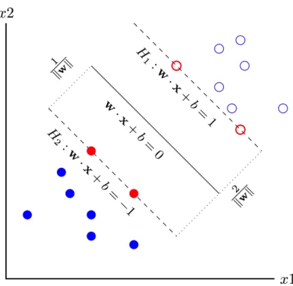
The problem of finding the optimal hyperplane is an optimization problem. Figure3.1illustrates an SVM classifier. In this figure, there are many possible hyperplanes, but the solid black line is the one that maximizes the margin (the distance between the hyperplane and the nearest data point of each class). The dashed lines identify the optimal separating hyperplanes with the largest margin. The selected data points nearest to the possible separating hyperplanes for a given training set are termed support vectors (SVs) (Steinwart and Christmann,2008). The SVs are points of a data set that, if removed, would alter the position of the optimal separating hyperplane.

(19)

Figure 3.1: How SVMs linearly classify data in a two-dimensional space

In technical terms, an SVM classifier for training examples labeled as belonging to two classes maps the input vectorsxi∈Rn,i= 1,2, . . . , m, into a higher-dimensional feature space and maximizes the margin (Xu

et al.,2009). The given data points take the form

{(x1, y1),(x2, y2),(x3, y3), . . . ,(xm, ym)},

where yi =±1 is the classification variable. For example, the class label +1 may correspond to a person who has gone missing on more than one occasion (missing_again) and the class label−1may correspond to those who have not.

The margin is defined as the distance of the hyperplane to the nearest of the positive and negative data points. The optimal hyperplane formula takes the form

w·x+b= 0,

where the weight vector w is the normal vector to the hyperplane. The optimal hyperplane can scale the length of w to force the closest point in the positive area to have inner product1 and the closest point in the negative area to have inner product−1. So, the supporting hyperplanes can be written as:

(20)

The two inequalities in (3.1) can be combined into one equation as:

yi(w·xi+b)≥1. (3.2)

Equation3.2is called the functional margin and defines whether a training sample is properly classified. Now consider in Figure 3.1 the SVs that lie on the hyperplanes, H1 and H2, which are parallel to the

optimal hyperplane.

Geometrically, the distance between these two hyperplanes is _k_w2_k. So, to define an optimal hyperplane we need to maximize the width of the margin. The margin mcan be defined asm= _k_w1_k. In other words, to maximize the marginm, we can minimizekwk. So, we can formulate the optimization problem as:

min1 2kwk

2_. _(3.3)

The general method to solve this problem is calledquadratic programmingoptimization (Chang and Lin,

2011).

In the case where the data do not offer linearly separable problems in the input space, they can become linearly separable problems via a nonlinear mapping into a higher-dimensional space. Nonlinear SVMs can be realized by the kernel mapping method to simulate a nonlinear projection of data into a higher-dimensional space where the classes are linearly separable (Mercier and Lennon,2003). When data are linearly separable, the linear classifier is used to find a perfect classifier. To find a perfect classifier, every data point (xi, yi) satisfies the functional margin (3.2). If the data are not linearly separable, SVM can use “slack” variables that allow constraint violations. The algorithm then attempts to minimize the misclassified data using the slack variables as follows:

min w,b,ξi 1 2kwk 2_{+ 1 +}_C m X i=1 ξi !

, subject to yi(w·φ(xi) +b)≥1−ξi ξi≥0. (3.4) In Equation (3.4), a slack variable is used to penalize all classification mistakes made in the training. The minimization in Equation (3.4) tries to balance the best of both worlds: maximizing the separation of classes while minimizing the amount of misclassification. Figure 3.2 shows an example of misclassified data using theξi variables.

(21)

Figure 3.2: Misclassified data using theξi variables

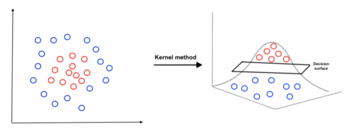
The simplest way to separate two groups of data is with a hyperplane. However, there are situations where a nonlinear surface can more efficiently separate the groups. Kernel methods are the way to provide a maximized margin and support nonlinear separation (Yu et al., 2003). SVMs are regarded as an active field of machine learning and have been the main application of kernel methods. Kernel methods map input data points into a higher-dimensional space. Figure 3.3 shows an example of mapping data into a higher-dimensional space using a kernel method.

Figure 3.3: Visualization of mapping data in a higher-dimensional space using a kernel method

Kernel methods attempt to allow us to perform linear classification on nonlinear features of the data without explicitly generating the features. Choosing a kernel method depends strongly on the data spec-ifications (Awad and Khanna, 2015). A great number of kernels exist, and they are categorized into two types: local kernelsand global kernels. With local kernels, kernel values can be affected only by the nearest

(22)

data points. However, with global kernels, kernel values can affected by the faraway data points too (Smits and Jordaan, 2002). In the nonlinear SVM, the n-dimensional input x are implicitly transformed into a (higher) ˜n-dimensional feature space using a transformation function (φ), a procedure that is called the kernel trick (Schölkopf,2001).

The kernel trick can be applied to nonlinear data to make them linearly separable. The ultimate goal of the model is to find a transformation function that creates(φ(xi), yi)in a new feature space with a separable hyperplane. In the new feature space, we have:

w·φ(xi) +b≥1.

then we can find an optimal separating hyperplane by solving the optimization problem in the new feature space.

There are four most common SVM kernel methods. The first kernel is thelinear kernel, which is regarded as a simple and useful method for classification and regression in large group of support vectors, defined as k(xi,xj) = (xi·xj). Figure3.4illustrates some contours of the linear kernel and shows that it can separate data linearly with a single line in a feature space (Schölkopf,2001).

Figure 3.4: Visualization of SVM linear kernel

The second kernel is the polynomial kernel, widely used in image processing and defined as k(xi,xj) = (γxi·xj+C)

n

, γ >0, whereγandCare the regularization parameters that are chosen via validation, andn is a dimensional parameter. Figure3.5illustrates some contours of the polynomial kernel (Schölkopf,2001).

(23)

Figure 3.5: Visualization of SVM polynomial kernel

The third kernel is theradial basis function(RBF) kernel, defined ask(xi,xj) = exp(−γ||xi−xj||2), γ > 0. The γ parameter defines how far the influence of a single training example reaches. The value of γ is chosen by the LIBSVM package as default value. Figure3.6illustrates the RBF kernel (Schölkopf,2001).

Figure 3.6: Visualization of SVM radial basis function kernel

The fourth kernel is the sigmoid kernel, mostly used for neural networks. The sigmoid kernel is the least popular kernel because of its poor performance (Ren et al., 2016). The sigmoid kernel is defined as k(xi,xj) = tanh(γxi·xj+c), where γ andc are regularization parameters that are chosen via validation. Figure3.7 illustrates contours of the sigmoid kernel (Schölkopf,2001).

(24)

Figure 3.7: Visualization of SVM sigmoid kernel

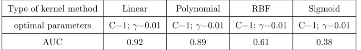
One way to choose an appropriate kernel and kernel parameters is through cross-validation. In the SVM kernel methods, the parameter C is a regularization term, which provides a way to control overfitting. The reverse defines how far the influence of a single training example reaches. The values ofC andγ are chosen by the LIBSVM package as default values. Table 3.1provides a comparison of different kernel methods for the MY Database. The results show the linear kernel method performs better than the other kernel methods for the MY database for the specific default values of theC andγparameters.

Type of kernel method Linear Polynomial RBF Sigmoid

optimal parameters C=1;γ=0.01 C=1;γ=0.01 C=1;γ=0.01 C=1;γ=0.01

AUC 0.92 0.89 0.61 0.38

Table 3.1: Comparison of different kernel functions for the MY database

In the linear SVM classification model, sometimes over-fitting problems occur when the sample data size is too small. The CV method is used to deal with over-fitting problems. The linear SVM works best when the data contain a small number of features. The10-fold CV function is performed as a method to find the best model using LIBSVM. Section 3.3.2provides a description of how CV was used in this study.

3.1.1

Linear SVM Classification Algorithm

(25)

python package. The Scikit-Learn package is designed as a machine learning library for the numerical and scientific Python programming libraries (Pedregosa et al.,2011). The Scikit-Learn package contains built-in classes for different SVM classification models. A basic structure of how to build and use an SVM is given in Algorithm 1(Hsu et al.,2003;Chang and Lin,2011).

Algorithm 1 Linear SVM classification model for specific case of two classes

1: procedure_{Linear SVM}(data)

2: Structure the data into features and class labels{(x1, y1),(x2, y2), . . . ,(xn, yn)}. 3: Divide the data into training and testing sets.

4: Define an optimal hyperplane using SVC: maximize margin.

5: (If the hyperplane cannot separate data linearly) Extend the linear classification definition for non-linearly separable problems: have a penalty term for misclassifications.

6: (If the hyperplane cannot separate data linearly) Map data to higher-dimensional space where it may be easier to classify with linear classifier: reformulate problem so that data are mapped to this space.

7: Validate the model by computing the percentage of correct classifications, etc., on the testing set.

Algorithm1 describes the process used to build and use an SVM predictive model. The first step (line 2) is to structure the data into features and class labels. For example, all the columns of the data are stored in thexvariable except formissing_againandgang_involvement, which are used as class labels and stored in they variable for the two different analyses performed. The second step (line 3) is to divide the data into two data sets, the training data set used for building the model and the testing data set used for validating the model. The third step (line 4) is to define an optimal hyperplane using SVC from the training data set. In practice, this is performed by finding the maximum margin hyperplane. If the hyperplane cannot separate data linearly, the fourth step (line 5) is to have a penalty term for the misclassified data points. If the hyperplane cannot separate data linearly, the fifth step (line 6) is to map nonlinearly separable data in a higher-dimensional feature space to classify with a linear classifier. The sixth step (line 7) is to validate the predictive capability of the model by, for example, computing the percentage of correct classifications (true positives) or accuracy (Azadeh et al., 2013). For a more detailed step-by-step breakdown of the process of building SVMs, see (Hsu et al., 2003).

3.2

Model Performance Evaluation

After training and validation of the model, the next step is to find out how effective the model is in terms of its performance on a test set. Different metrics are used to evaluate the performance of a model (Muller and Guido,2017). The following sections focus on the metrics used in this study to estimate the performance of the constructed models.

(26)

3.2.1

Confusion Matrix

The performance of a classifier can be visualized by a matrix known as the confusion matrix (Kononenko and Kukar, 2007). The rows and columns of the confusion matrix present observed and predicted class labels, respectively. The confusion matrix for a class feature with two unique values of 1 and 0 is

Predicted Value Observed

Value

True Positive (TP) = 11 False Negative (FN) = 10 False Positive (FP) = 01 True Negative (TN) = 00

Table 3.2: A confusion matrix

where 1≡Positive, 0≡Negative, true positive (TP) is the number of testing instances observed in class1 that are correctly predicted to be in class 1, false negative (FN) is the number of testing instances observed in class1that are incorrectly predicted to be in class0, true negative (TN) is the number of testing instances observed in class0that are correctly predicted to be in class0, and false positive (FP) is the number of testing instances observed in class0 that are incorrectly predicted to be in class1. Using the confusion matrix, one can easily obtain the accuracy and some other performance measures such as sensitivity and specificity in terms of the entries of the confusion matrix as follows.

3.2.2

Accuracy

The accuracy of a model tells us that what portion of the testing data is correctly classified. In terms of confusion matrix elements, accuracy is defined by the following formula

A= TP + TN

TP + TN + FP + FN, (3.5)

where the numerator is the total number of correctly predicted outcomes, and the denominator is the total number of instances.

3.2.3

Sensitivity and Specificity

The sensitivity or true positive rate (TPR) and the specificity or true negative rate (TNR) are two other measures that show to what extent a classifier is correct in classifying testing data as positive and to what extent all positives are classified correctly (Costa et al.,2007). The sensitivity and specificity are defined by

(27)

The false positive rate (FPR) is the number of cases incorrectly predicted as positive. The false negative rate (FNR) is the number of cases incorrectly predicted as negative.

3.2.4

Receiver Operating Characteristic Curve

The Receiver Operating Characteristic (ROC) curve is a tool that commonly used to illustrate the perfor-mance of a binary classifier (Carter et al., 2016). In World War II, the British Royal Air Force developed a ROC curve method for the radar signal detection and to find the different signals of interest (Carter et al.,

2016). The ROC curve is a graphical plot that illustrates the diagnostic ability of a binary classifier system as its discrimination threshold is varied. It is created by plotting the (TPR) (sensitivity) against the (FPR) (1 −specificity) at various threshold settings. The area under the ROC curve (AUC) can be used to com-pare the performance of multiple classifiers. A classifier with a higher AUC has better performance. The recommended tool for the accuracy in statistical analysis is the AUC (DeLong et al.,1988).

Using the data from the MY database, a statistical model was developed to predict from whether a missing youth is likely to go missing again or whether a missing youth is likely to have gang affiliations.

3.3

Model Validation

In general, a predictive model can be validated in various ways. In the following sections, the two methods of simple split and cross-validation employed in the construction of each predictive model in this study as validation methods are briefly reviewed.

3.3.1

Simple Split

In the simple split method, the original data are randomized and split into two groups, 80%for the training set and20%for the testing set. In this method, the samples are selected with uniform distribution, meaning that each sample has the same probability for being selected (Qiang and Zhongli,2011).

3.3.2

Multi-fold Cross-validation

Cross-validation is the method that results in the best selection of the hyper-parameters compared to the other split methods, but for a large database, it may have a high execution time. One way to reduce risk of over-fitting is to use a multi-fold CV process, so a model is not simply over-fit to a training subset. Particularly given the large number of features considered, there is a higher likelihood of over-fitting, and it is not acceptable to simply use one designated subset for training and another for testing. In this thesis, a CV is used as a re-sampling method. This method refits a model of interest as samples formed from the training set in order to obtain additional information about the fitted model. For example, it can provide estimates of test-set prediction error, and the standard deviation and bias of the parameter estimates.

(28)

CV is a statistical method that aims at minimizing the probability of over-fitting and creating a more unbiased model (Kononenko and Kukar, 2007; Refaeilzadeh et al., 2009). Another goal of CV is to select the best model among different training algorithms (Reitermanov,2010). Also, CV can be used to find the optimal parameters of models with different levels of complexity (Reed and Marks,1998), such as Random Forest Classifications with different depths or number of Decision Tree Classifications in the forest. CV has many methods, but k-fold CV is the most popular one (Murphy, 2012). The reason for the popularity of k-fold CV is that all observations are used for both training and validation. In addition, each observation is used exactly once for validation. So, it is helpful to reduce overfitting.

In the k-fold CV method, the original data are divided into k subsets with nearly equal sizes. For example, the MY database contains434observations divided into10folds. So, there are6folds that contain 43observations and4 folds that contain44observations. In k-fold CV,k−1subsets form the training set, and the remaining subset forms the validation set. The model is trained based on the training set for a total of ktimes, and the prediction error is estimated using the validation set. This process is repeated for each subset, and the average of the prediction error values is determined using

E(i) = Pk

j=1Ej

k .

The main disadvantage ofk-fold CV is that depending on the value ofk, this method can be computa-tionally expensive (Muller and Guido,2017). The choice of the number of folds depends on the computation time and the number of samples in the data. With a larger value ofk, the error estimation tends to be more accurate, but the process can be computationally expensive. Usually, researchers choose k = 10, but for a large number of samples it is better to choose a smaller value for k in order to decrease the computation time (Reitermanov,2010). In this thesis, a combination of both methods of simple split and10-fold CV can be used by the following steps (Ozkan,2017;Hastie et al.,2008):

Step 1: Split the randomized original data into training and testing sets.

Step 2: Use k-fold CV on the training set to build the model. In this step, by considering the least average prediction error on the test set, the best parameters for the model can be chosen.

Step 3: Evaluate the model performance using the testing set.

3.4

Description of the MY Database

The purpose of this section is to describe a set of theoretical and empirical risk factors surrounding different aspects of MY investigations, a description of each feature found within the tables in the MY database, and

(29)

variety of other features associated with missing youth and their cases were pulled (using an SQL query) from all available tables to make up the missing youth data set. All other available data from the MY database were used to ensure no bias was introduced by preselecting features by hand. The code used to query the MY data is written in mySQL (Greenspan and Bulger,2001). The final step to build a predictive model was to encode the output data to a binary value. This does not change what the data represent but rather only changes the format in which they are presented and allows for easier manipulation within the algorithm.

The final data set contained434missing youths cases reported between September27,1971, and February 18, 2016, with91 distinct features. The feature missing_again contains 171 instances of youth who went missing more than once (and accordingly, 263 instances of youth who only went missing once). The feature gang_involvement contains 71 instances of youth with suspected gang involvement (and accordingly 363 instances of no suspected gang involvement). The full extent of the features cannot be disclosed due to confidentiality.

3.4.1

Classification Features

In this thesis, a missing person is a person who has been formally reported to the police as someone who has gone missing. In 2016, Bonny et al. in their research indicate that the personal behaviours of a youth and family violence are the main reasons for youths to go missing or run away. The actual number of missing youths cases is lower than the number of missing youths reporting files. This indicates that some cases are for youths who go missing more than once in a year (Pfeifer,2006).

Youth gang involvement is also a serious problem for many law enforcement agencies in the United States. More than one million youths are involved in gang in the United States every year (Walters,2019). Youths at risk of running away are more likely to engage in gang affiliations.

Based on the studies (Bonny et al.,2016; Pfeifer, 2006;Walters, 2019), the classification features miss-ing_againandgang_involvementare respectively chosen to build predictive models to indicate when a youth is likely to go missing again and is likely to be involved in gang activity. It is also important to identify the features that could be most important to answering those two questions. The predictive models are trained by the classification features. In this section, the two classification features that are used to build the predictive models for the MY database are presented.

The first classification feature ismissing_again. If a youth has gone missing more than once, this feature has a value of 1, otherwise it has a value of 0. Using missing_again as a classification feature allows us to train a predictive model to predict whether or not a youth is likely to go missing again. The second classification feature isgang_involvement. If a youth is believed to havegang_involvement, this feature has a value of 1, otherwise it has a value of 0. Using gang_involvementas a classification feature allows us to train a predictive model to predict whether or not a missing youth is likely to be involved in gang activity. These classification features along with 91features associated with the MY and their case are merged into one table that is used to train the predictive model.

(30)

3.5

Graphical User Interface Development

This section provides the process of the design and development of the MY GUI. The main concept of the MY GUI is to provide a visual grouping of data with minimal effort required regarding user actions.

3.5.1

Missing Youths Graphical User Interface Development

A GUI provides a user-friendly environment featuring elements, such as menus, buttons, text boxes, and lists, for easy access for the end users. However, a GUI can be complex and hard to develop, debug, and modify for the programmer. A programmer can attract users by creating a strong interaction between front-end and back-end design. In order to have a desirable visualization, a GUI needs to be beautiful and functional. The front-end design is a visualization for the programmer to divide the design and development worlds. GUI development requires that the programmer deal with created graphics and multiple ways of giving the same commands to the input devices. The important point of GUI development is to pay extensive attention to the needs and limitations of the end users.

GUI development can be divided into five high-level steps. The first step is to analyze the user needs. The second step is to create a development plan and find a possible path of development. This step involves a schematic image of the screens, linked together through a visual service. The third step is to find an appropriate platform. During the GUI development, different platforms lead to different tools. For instance, for a web-based application, design tools such as HTML, JavaScript, and .css are common. The fourth step is to evaluate the GUI. The main goal of this step is to verify that the GUI meets the needs of the users. The fifth step is to determine if the GUI is complete. The process of GUI development is stopped when the evaluation process is no longer generating any new requirements, or a small number of relatively unimportant requirements (Bischofberger and Pomberger,2012).

There has been significant progress in software tools to help with creating a GUI. The MY GUI structure is programmed in the Python programming language using a Python template engine called Jinja2 (Ronacher,

2008). Python is a high-level programming language that focuses on code readability for web-based develop-ment. Python has a large number of web libraries and frameworks that make development of code short and simple (Lokhande et al.,2015).

The MY GUI is built by the CherryPy object-oriented web framework (Hellegouarch,2007). CherryPy is a Python library providing a GUI to the HTTP protocol. CherryPy was chosen because of its simplicity, self-containment, and non-intrusiveness. The program is easily able to narrow and expand the coverage of the libraries, and it is an independent module that can be designed by developers (Shinde and Patel,2014). The

(31)

In this appendix, a mock database is used for demonstration purposes because the MY database is a secure data set.

3.5.2

Logical Diagram

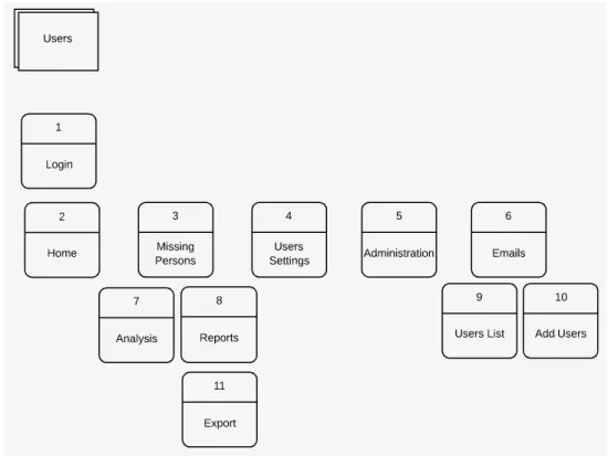
The logical diagram for the MY GUI represents information gathered from the SPS requirements. Developing a logical diagram for the MY GUI affords a clear understanding of how the GUI operates. The MY GUI can be a lightweight web application, where all functionality is grouped visually and logically into thematic units. The benefit of the logical diagram for the MY GUI is that it is more easily understandable to non-technical people. Figure3.8represents the logical diagram for the MY GUI.

Figure 3.8: Logical diagram for the MY GUI

3.5.3

Physical Diagram

The logical development of a GUI is used to create a physical diagram of the system. The physical diagram shows the structure of possible navigation paths and connections and the system functionality through the GUI. In the MY GUI development, the logical and physical diagrams both contain entities and relationships, but they differ in the purposes for which they are created and the audiences they are meant to target. The physical diagram of the MY GUI can be seen in Figure3.9.

(32)

Figure 3.9: Ph ysical diagr am of the MY GUI

(33)

Chapter 4

Results

The results of some data analysis including the SVM classifier is discussed in this chapter. The MY database contains434MY cases records with95features. It is valuable to use some features such as surname, g1 (first name), g2 (middle name), and dob (date of birth) from the MY database to determine unmatched MY cases. For example, a shared family name can give indications as to gang affiliation beyond for a single case. Table4.1contains some descriptive statistics about the MY cases.

Total Male Female Missing Again Gang Involvement

434 155 279 171 71

Table 4.1: Basic information about the MY cases

4.1

Basic Statistical Analysis of the Missing Youths Database

Repeat missing youths are an important issue for the Ministry of Justice of Saskatchewan and the SPS. In this section, some basic descriptive statistical analysis, e.g., means, standard deviations, modes, and medians, are provided for the samples of the MY database.

The focus on MY data is to find out the MY cases age groups, missing period, occurrences, and the time to the next event for each gender. These statistical analyses can provide a significant amount of information to contribute to addressing MY issues. The age of each MY is calculated based on the difference between their date of birth from the dob column and the date from the date_missing column in the MY database. The results are shown in Table4.2. The mean age of the MY is 13.8years with a standard deviation of 3.2 years, and the mode and median age of the MY are both 15years.

Mean Standard Deviation Mode Median

13.8 3.2 15 15

(34)

Figure 4.1 gives a histogram of the ages for the people at the centre of the MY cases, from which we observe a high number of cases involving teenagers.

Figure 4.1: Histogram of age

Table 4.3 shows the mean, standard deviation, mode, and median results for male and female missing youth in different age groups. The most common (mode) age of missing youths for males is13years and for females it is15years.

Gender Mean Standard Deviation Mode Median

Male 13 3.9 13 14

Female 14.2 2.6 15 15

Table 4.3: Basic statistics for age grouped by gender (years)

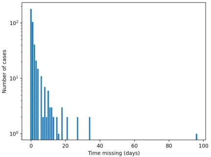
The time missing for each MY is calculated based on the difference between the date from thedate_located column and the date from thedate_missingcolumn in the MY database and excluded the cases where there was no date_located. The results are shown in Table4.4. The mean of the time missing is3.1 days with a standard deviation of 7.7 days, and the mode and median age of MY are0 (less than24hours) and 1 day, respectively. The MY database has around 30%of missing cases that do not have adate_locatedentry.

(35)

Figure4.2gives a semi-log histogram of the time missing for the number of the MY cases, from which we observe a high number of cases are resolved within one day (24hours).

Figure 4.2: Histogram of time missing

Table 4.5 shows the mean, standard deviation, mode, and median results for time missing grouped by gender. The most common time missing for both males and females are less than a day, indicating that most missing youths are found within24hours.

Male 2.8 6.6 0 1

Female 3.3 8.2 0 1

Table 4.5: Basic statistics for time missing grouped by gender (days)

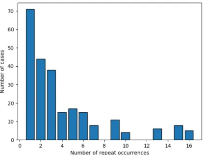
The average number of repeat events of each incident of a missing youth is calculated based on the missing_again column in the MY database. The results are shown in Table 4.6. The mean of the repeat events is 4times with a standard deviation of 3.8 times, and the mode and median age of MY are2 and4 times, respectively.

4 3.8 2 4

Table 4.6: Basic statistics for repeat occurrences (number of times)

Figure4.3gives a histogram of the repeat events for the number of the MY cases, from which we observe a high number of youths who are reported missing twice.

(36)

Figure 4.3: Histogram of repeat occurrences

Table4.7shows the mean, standard deviation, mode, and median results for repeat occurrences grouped by gender. The most common number of the repeat events for males is1 time and for females it is2 times.

Male 3.3 1.5 1 3

Female 5.7 4.3 2 4

Table 4.7: Basic statistics for repeat occurrences grouped by gender (number of times)

The time to the next event of each MY is calculated based on the missing_again, surname, g1 (first name),g2(nickname), and date_locatedcolumns in the MY database. In this analysis,g1,g2, andsurname of each case are required to make sure that different nicknames are not used in different occurrences. The results are shown in Table4.8. The mean of the time to the next event is584days (1.6years) with a standard deviation of511days (1.4 years), and the mode and median age of MY are73days (0.2 years) and401 days (1.1 years), respectively. In this analysis, there are two different situations for missing youth cases that do not have any next event. The first situation is that a youth ages out of the youth age category. In this case, there is no more information about the case. The second situation is that a missing youth case has not gone missing or run away again. To handle these situations, each case which does not contain date_locatedhas

(37)

584 511 73 401

Table 4.8: Basic statistics for time to the next event (days)

Figure 4.4: Histogram of time to next event

Table 4.9 shows the mean, standard deviation, mode, and median results for time to the next event grouped by gender. The most common time to the next event for males is58 days and for females it is 98 days. Based on the repeat occurrences result, female missing cases are repeated two times more than those for males.

Male 511 547 58 368

Female 620 1460 98 730

Table 4.9: Basic statistics for time to the next event grouped by gender (days)

4.2

Missing Youths Experiment Results

In subsections4.2.1and 4.2.2, the results of the SVM classifier accepting a combination of 91 input features for each MY case from the MY database as input andmissing_againandgang_involvementas two classification features are discussed. The results for the SVMs have been measured according to accuracy, sensitivity, specificity, FNR, and FPR. The SVM classifier was able to obtain an 89% accuracy for themissing_again

(38)

classification feature and an 84%accuracy for the gang_involvementclassification feature.

4.2.1

Results for the missing_again classification feature

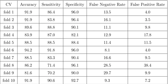
Table 4.10shows the results for the SVMs applied to the MY database for the missing_againclassification feature with the simple split and the10-fold CV method. The sample size of youths who go missing more than once is171out of the total434cases, and accordingly there are263instances of youth who go missing only once.

In the10-fold CV method, the training set is broken down randomly into10 folds. For each validation, the first fold is treated as a testing set and the model is fit on the remaining9 folds. Based on the results, the accuracies are in the range of82%for fold9as testing set to94%for fold6as testing set. Also, the FNR are in the range of8%for fold6 as testing set and30% for fold9 as testing set. In this case, fold6has been selected as leading to the best model because it has the highest accuracy and low FNR in the training set. Looking at the results produced for themissing_again classification feature in Table4.10, the SVM model was able to obtain high accuracies and high sensitivities using the 10-fold CV. The higher numerical value of sensitivity indicates the low likelihood of diagnostic false-positive results. So, we conclude that the linear SVM classifier model is a model with relatively few misclassified data points for the MY database.

CV

Accuracy

Sensitivity

Specificity

False Negative Rate

False Positive Rate

fold 1

91.9

86.4

96.0

13.5

4.0

fold 2

91.9

83.8

96.4

16.1

3.5

fold 3

89.6

88.8

90.1

11.1

9.8

fold 4

83.9

87.0

82.1

12.9

17.8

fold 5

88.5

88.4

11.4

11.5

fold 6

94.2

91.8

96.0

8.1

4.0

fold 7

88.5

83.3

90.4

16.6

9.5

fold 8

86.2

71.4

96.1

28.5

38.4

fold 9

81.6

70.2

90.0

29.7

9.9

fold 10

91.9

90.6

92.7

9.3

7.2

(39)

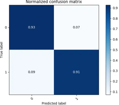
Figure 4.5, the classification performance of the missing_again classifier is summarized using a confusion matrix. According to the normalized confusion matrix of themissing_again classifier, the TPR is93, which means 93% of youth in this class are correctly predicted as who have gone missing. The FNR is 7, which means7%of youth in this class are incorrectly predicted as who have gone missing. The TNR is 91, which means91% of youth are correctly predicted as who have not gone missing. The FPR is9, which means9% of youth are incorrectly predicted as who have not gone missing.

Figure 4.5: Confusion matrix for the missing_againclassification feature

4.2.1.2 ROC Curve for the missing_again Classification Feature

Figure4.6refers to the diagnostic performance of the accuracy of a test to discriminate where youths are at a high risk to go missing again. In this figure, the area under curve is equal92%; we consider this to be good at separating youth who have gone missing more than once from youth who have not. The correct positive results represent the values plotted above of the equality line (denoted by the dotted green line).

(40)

Figure 4.6: Receiver Operating Characteristic curve for themissing_againclassification feature

4.2.2

Results for the gang_involvement Classification Feature

Table4.11shows the results for the SVMs applied to the MY database for thegang_involvementclassification feature with the simple split and the10-fold CV. There are the sample size of youths who were suspected of gang involvement is71out of the total434cases, and accordingly there are363instances of youth who were not suspected of gang involvement.

In the10-fold CV method, the training set is broken down randomly into10 folds. For each validation, the first fold is treated as a testing set and the model is fit on the remaining9folds. When9of those folds are used as the training data set, relatively few samples remain for testing. This would lead to greater variability in the estimates. Based on the results, the accuracies are in the range of79% for folds1 as testing set and 3 to 87% for folds 4 and10 as testing set. Also, the FNR are in the range of 36% for fold 4 as testing set and 71% for fold 1 as testing set. So, fold 4 has been selected as leading to the best model because it has the highest accuracy and a relatively low FNR in the training set. Looking at the results produced for the gang_involvementclassification feature in Table4.11, the SVM model was able to obtain high accuracies but low sensitivities using the10-fold CV. The lower numerical value of sensitivity indicates the high likelihood of diagnostic false-positive results.

(41)

SVMs

Accuracy

Sensitivity

Specificity

False Negative Rate

False Positive Rate

fold 1

79.3

28.5

89.0

71.4

10.9

fold 2

86.2

56.2

92.9

43.7

7.0

fold 3

79.3

45.4

84.2

54.5

15.7

fold 4

87.3

64.2

91.7

35.7

8.2

fold 5

80.4

47.0

88.5

52.9

11.4

fold 6

82.7

33.3

90.

Classification of Missing Youths Cases using Support Vector Machines