Inferring the geolocation of tweets at a fine-grained level

(1)

Gonzalez Paule, Jorge David (2019) Inferring the geolocation of tweets at a

fine-grained level. PhD thesis.

https://theses.gla.ac.uk/41007/

Copyright and moral rights for this work are retained by the author

A copy can be downloaded for personal non-commercial research or study,

without prior permission or charge

This work cannot be reproduced or quoted extensively from without first

obtaining permission in writing from the author

The content must not be changed in any way or sold commercially in any

format or medium without the formal permission of the author

When referring to this work, full bibliographic details including the author,

title, awarding institution and date of the thesis must be given

(2)

Inferring the Geolocation of Tweets

at a Fine-Grained Level

Jorge David Gonzalez Paule

School of Computing Science

University of Glasgow

Submitted in fullment of the requirements for the Degree of

Doctor of Philosophy (PhD)

(3)

ers, the contents of this dissertation are original and have not been submitted in whole or in part for consideration for any other degree or qualication in this, or any other University.

This dissertation is the result of my own work, under the supervision of Professor Iadh Ouinis, Dr Craig MacDonald and Dr Yashar Moshfeghi, and includes noth-ing which is the outcome of work done in collaboration, except where specically indicated in the text.

Permission to copy without fee all or part of this thesis is granted provided that the copies are not made or distributed for commercial purposes, and that the name of the author, the title of the thesis and date of submission are clearly visible on the copy.

Jorge David Gonzalez Paule February, 2019

(4)

(5)

Abstract

Recently, the use of Twitter data has become important for a wide range of real-time applications, including real-real-time event detection, topic detection or disaster and emergency management. These applications require to know the precise lo-cation of the tweets for their analysis. However, approximately 1% of the tweets are nely-grained geotagged, which remains insucient for such applications. To overcome this limitation, predicting the location of non-geotagged tweets, while challenging, can increase the sample of geotagged data to support the applications mentioned above. Nevertheless, existing approaches on tweet geolocalisation are mostly focusing on the geolocation of tweets at a coarse-grained level of granular-ity (i.e., cgranular-ity or country level). Thus, geolocalising tweets at a ne-grained level (i.e., street or building level) has arisen as a newly open research problem. In this thesis, we investigate the problem of inferring the geolocation of non-geotagged tweets at a ne-grained level of granularity (i.e., at most 1 km error distance). In particular, we aim to predict the geolocation where a given a tweet was generated using its text as a source of evidence.

This thesis states that the geolocalisation of non-geotagged tweets at a ne-grained level can be achieved by exploiting the characteristics of the 1% of al-ready available individual nely-grained geotagged tweets provided by the Twit-ter stream. We evaluate the state-of-the-art, derive insights on their issues and propose an evolution of techniques to achieve the geolocalisation of tweets at a ne-grained level.

First, we explore the existing approaches in the literature for tweet geolocal-isation and derive insights on the problems they exhibit when adapted to work at a ne-grained level. To overcome these problems, we propose a new approach that ranks individual geotagged tweets based on their content similarity to a given

(6)

non-geotagged. Our experimental results show signicant improvements over pre-vious approaches.

Next, we explore the predictability of the location of a tweet at a ne-grained level in order to reduce the average error distance of the predictions. We postu-late that to obtain a ne-grained prediction a correlation between similarity and geographical distance should exist, and dene the boundaries were ne-grained predictions can be achieved. To do that, we incorporate a majority voting algo-rithm to the ranking approach that assesses if such correlation exists by exploit-ing the geographical evidence encoded within the Top-N most similar geotagged tweets in the ranking. We report experimental results and demonstrate that by considering this geographical evidence, we can reduce the average error distance, but with a cost in coverage (the number of tweets for which our approach can nd a ne-grained geolocation).

Furthermore, we investigate whether the quality of the ranking of the Top-N geotagged tweets aects the eectiveness of ne-grained geolocalisation, and propose a new approach to improve the ranking. To this end, we adopt a learning to rank approach that re-ranks geotagged tweets based on their geographical proximity to a given non-geotagged tweet. We test dierent learning to rank algorithms and propose multiple features to model ne-grained geolocalisation. Moreover, we investigate the best performing combination of features for ne-grained geolocalisation.

This thesis also demonstrates the applicability and generalisation of our ne-grained geolocalisation approaches in a practical scenario related to a trac inci-dent detection task. We show the eectiveness of using new geolocalised inciinci-dent- incident-related tweets in detecting the geolocation of real incidents reports, and demon-strate that we can improve the overall performance of the trac incident detection task by enhancing the already available geotagged tweets with new tweets that were geolocalised using our approach.

The key contribution of this thesis is the development of eective approaches for geolocalising tweets at a ne-grained level. The thesis provides insights on the main challenges for achieving the ne-grained geolocalisation derived from exhaustive experiments over a ground truth of geotagged tweets gathered from two dierent cities. Additionally, we demonstrate its eectiveness in a trac

(7)

incident detection task by geolocalising new incident-related tweets using our ne-grained geolocalisation approaches.

(8)

Acknowledgements

My research would have been impossible without the aid and support of my supervisors, Prof. Iadh Ounis, Dr Craig MacDonald and Dr Yashar Moshfeghi. I am profoundly thankful for their patience, motivation, and immense knowledge. I could not have imagined having better advisors and mentors. Thanks also to my examiners, Dr Richard McCreadie and Prof. Mohand Boughanem for their insightful comments and corrections to improve this thesis.

Special thanks to Dr Yashar Moshfeghi for being my mentor and helping me shape my research ideas. He provided me through moral and emotional support in the hardest moments, and always had the right words to guide me through this adventure. For that, I will be forever thankful.

I would also like to acknowledge my fellow doctoral students for their cooper-ation and friendship. With a special mention to those with whom I have shared an oce. Such as David Maxwell, Stuart Mackie, Jarana Manotumruksa, Fatma Elsafoury, Colin Wilkie, Rami Alkhawaldeh, Stewart Whiting, Fajie Yuan, James McMinn and Phil McParlane. It has been a pleasure!

Also, my sincere thanks to the persons who helped me in dierent ways during this endeavour, and all the extraordinary people that I had the privilege to meet during my ve years in Glasgow. With special mention to Jesus Rodriguez Perez for encouraging me to start this adventure, and for his invaluable help, support and the moments we shared living together.

I dedicate this thesis to my parents, Nieves Maria Paule Rodriguez and Jorge Luis Gonzalez Garcia, to my grandparents, Maria Jose Rodriguez Darias and Francisco Paule Rodriguez, and to my great grandparents in heaven, Ramon Rodriguez Rodriguez and Nieves Darias Hernandez. Without their innite love, support and sacrice, I would not have been to this far. I am lucky and proud of having you.

(9)

Finally, last but not least, I will always be grateful to my whole family and loved ones for always being there for me through thick and thin. To my aunts and uncles, Ana Belen Paule Rodriguez, Eduardo Sanson-Chirinos Lecuona, Maria Jose Rodriguez Darias and Venancio Nuñez Diaz. To my cousins, Victor Ruiz Paule, Raquel Moro Parrilla, Elena Chirinos Paule and Javier Sanson-Chirinos Paule.

(10)

II Fine-Grained Geolocalisation of Tweets

37

3 Enabling Fine-Grained Geolocalisation 38 3.1 Introduction . . . 38

3.1.1 Research Questions . . . 39

3.2 Modelling Tweet Geolocalisation . . . 40

3.2.1 Representing Candidate Locations . . . 40

3.2.1.1 Aggregated Approach . . . 40

3.2.1.2 Individual Approach . . . 41

3.2.2 Predicting a Geolocation . . . 41

3.3 Experimental Setting . . . 41

3.3.1 Data . . . 41

3.3.1.1 Training, Testing and Validation Sets . . . 43

3.3.2 Preprocessing and Indexing . . . 44

3.3.3 Models . . . 44

3.3.3.1 Aggregated . . . 44

3.3.3.2 Individual . . . 45

(12)

3.3.5 Parameter Tuning . . . 46

3.3.6 Evaluation Metrics . . . 47

3.4 Results and Discussions . . . 48

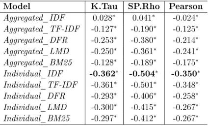
3.4.1 Aggregated Versus Individual . . . 49

3.4.1.1 The BM25 case . . . 51

3.4.2 Eect of Tweet Aggregation . . . 52

3.5 Chapter Summary . . . 55

4 Majority Voting For Fine-Grained Geolocalisation 58 4.1 Introduction . . . 58

4.1.1 Research Questions . . . 61

4.2 Related Work . . . 61

4.3 Voting For Fine-Grained Geolocalisation . . . 63

4.3.1 Majority Voting . . . 63

4.3.2 Weighted Majority Voting . . . 64

4.3.2.1 Extracting Credibility from a Tweet's User . . . . 65

4.3.2.2 Similarity Score and Tweet Geolocation . . . 66

4.4 Experimental Setting . . . 67

4.4.1 Models . . . 68

4.4.1.1 Baseline Models . . . 68

4.4.1.2 Majority Voting Model . . . 68

4.5 Experimental Results . . . 69

4.5.1 Performance of Fine-Grained Geolocalisation . . . 70

4.5.2 Eect of Weighting The Votes . . . 73

4.5.3 Comparing Behaviour Across Datasets . . . 74

4.6 Chapter Summary . . . 75

5 Learning to Geolocalise 78 5.1 Introduction . . . 78

5.2 Learning to Geolocalise . . . 80

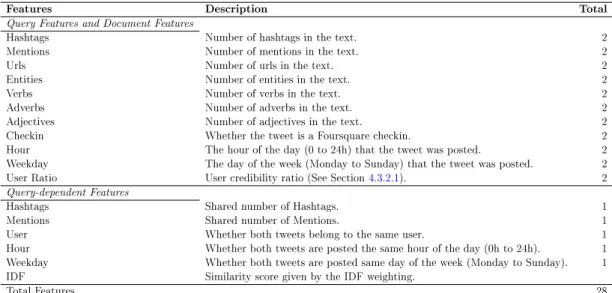
5.2.1 Feature Set For Fine-Grained Tweet Geolocalisation . . . . 80

5.2.1.1 Query Features and Document Features . . . 81

5.2.1.2 Query-Dependent Features. . . 82

(13)

5.3.1 Creating Training and Testing Sets for Learning to Rank . 83

5.3.2 Models . . . 84

5.4.1 Performance of Learning to Rank Algorithms . . . 87

5.4.2 Eectiveness on Fine-Grained Geolocalisation . . . 88

5.4.2.1 Applying Majority Voting . . . 92

5.4.2.2 Best Features for Fine-Grained Geolocalisation . 100 5.4.3 Comparing Behaviour Across Datasets . . . 101

5.5 Conclusions . . . 102

III Applicability

106

6 Eectiveness of Fine-Grained Geolocalised Tweets 107 6.1 Introduction . . . 107

6.2 Background . . . 108

6.3 Data . . . 110

6.3.1 Twitter Data . . . 110

6.3.2 Trac Incident Data . . . 112

6.4 Classication of Incident-Related Tweets . . . 113

6.4.1 Incident-Related Twitter Dataset . . . 113

6.4.2 Evaluation . . . 114

6.5 Fine-Grained Geolocalisation . . . 115

6.6 Trac Incident Detection . . . 117

6.6.1 Identifying Trac Incident-Related Tweets . . . 118

6.6.2 Applying Fine-Grained Geolocalisation . . . 120

6.6.3 Spatial Linking to Trac Incidents . . . 121

6.6.4 Evaluation Metrics . . . 121

6.7.1 Eectiveness of Geolocalised Tweets . . . 123

6.7.2 Expanding The Sample of Geotagged Tweets . . . 125

6.8 Recommendations to Transportation Managers . . . 126

(14)

IV Conclusions

131

7 Conclusions and

Future Work 132

7.1 Contributions . . . 133

7.2 Findings and Conclusions . . . 134

7.2.1 Limitations of State-of-The-Art Geolocalisation Approaches 135

7.2.2 Predictability of the Geolocation of Tweets at a Fine-Grained Level . . . 137

7.2.3 Improving The Quality of The Ranking for Fine-Grained Geolocalisation . . . 138

7.2.4 Eectiveness of The Fine-Grained Geolocalisation for Traf-c InTraf-cident DeteTraf-ction . . . 139

7.3 Future Research Directions . . . 141

A Fined-Grained Geolocalisation Models for Trac Incident

De-tection 143

B Detailed Results for Trac Incident Detection 147

B.1 Eectiveness of Geolocalised Tweets . . . 147

B.2 Expanding The Sample Of Geotagged Tweets . . . 148

(15)

List of Tables

2.1 A bag-of-words representation of a document. . . 14

2.2 Summary of the state-of-the-art Tweet geolocalisation approaches. 34

3.1 North-east (NE) and south-west (SW) longitude/latitude coordi-nates of the bounding boxes of the Chicago and New York datasets. 42

3.2 Number of geotagged tweets distributed between training, valida-tion and testing sets of the Chicago and New York datasets. . . . 43

3.3 Optimised parameters for the ranking functions used in Aggregated and Individual approaches on our two datasets, Chicago and New York. . . 47

3.4 Evaluation results for the Chicago dataset. The table presents the Average Error Distance in kilometres (AED), Median Error Dis-tance in kilometres (MED), Accuracy at 1 kilometre (Acc@1km) and Coverage. Signicant (statistically) dierences with respect to the best Baseline (Aggregated using BM25) are denoted by ∗

(p<0.01). . . 49

3.5 Evaluation results for the New York dataset. The table presents the Average Error Distance in kilometres (AED), Median Error Distance in kilometres (MED), Accuracy at 1 kilometre (Acc@1km) and Coverage. Signicant (statistically) dierences with respect to the best Baseline (Aggregated using BM25) denoted by ∗ (p<0.01). 50

3.6 Correlations between error distance and retrieval score. Signicant (statistically) dierences are denoted by ∗ (p<0.01). . . 54

(16)

4.1 Results for the Chicago dataset. The table presents the Aver-age Error Distance in kilometres (AED), Median of Error distance (MDE), Accuracy at 1 kilometre (A@1km) and Coverage for our proposed approach (WMV ) using the Top-N (@TopN ) elements in the rank and values of α, against the baselines. Additionally, we present results of the best performing models of Chapter 3, Aggregated and Individual. . . 71

4.2 Results for the New York dataset. The table presents the Aver-age Error Distance in kilometres (AED), Median of Error distance (MDE), Accuracy at 1 kilometre (A@1km) and Coverage for our proposed approach (WMV ) using the Top-N (@TopN ) elements in the rank and values of α, against the baselines. Additionally, we present results of the best performing models of Chapter 3, Aggregated and Individual. . . 72

5.1 Features extracted for ne-grained geolocalisation of tweets. . . . 81

5.2 Ranking performance for the Chicago dataset. The table presents NDCG@1, @3, @5 and @10 for the learning to rank algorithms and the baseline (IDF weighting). We run our experiment using all the features (All). A randomized permutation test was con-ducted to show signicant dierences with respect to the baseline (IDF), denoted by(p<0.01) for better performance,for worse

performance and =for no statistical dierence. . . 89 5.3 Ranking performance for the New York dataset. The table presents

NDCG@1, @3, @5 and @10 for the learning to rank algorithms and the baseline (IDF weighting). We run our experiment using all the features (All). A randomized permutation test was conducted to show signicant dierences with respect to the baseline (IDF), denoted by (p<0.01) for better performance, for worse

(17)

5.4 Fine-grained geolocalisation results for the Chicago dataset consid-ering only the Top-1. We compare our learning to rank approach (L2Geo) against the baseline (Individual using IDF). We report average error distance (AED), median error distance (MED), ac-curacy at 1 km (Acc@1km) and coverage (Coverage). We use a paired t-test to assess signicant dierences, denoted by for

better performance, for worse performance and =for no statis-tical dierence. . . 91

5.5 Fine-grained geolocalisation results for the New York dataset con-sidering only the Top-1. We compare our learning to rank ap-proach (L2Geo) against the baseline (Individual using TF-IDF). We report average error distance (AED), median error distance (MED), accuracy at 1 km (Acc@1km) and coverage (Coverage). We use a paired t-test to assess signicant dierences, denoted by

for better performance, for worse performance and =for no statistical dierence. . . 91

5.6 Fine-grained geolocalisation results for the Chicago dataset us-ing the majority votus-ing algorithm. We compare our approach (L2Geo+MV) against the baseline (MV) considering the Top-3, -5, -7 and -9 most similar geotagged tweets. Table reports average error distance (AED), median error distance (MED), accuracy at 1 km (Acc@1km) and coverage (Coverage). . . 93

5.7 Fine-grained geolocalisation results for the New York dataset us-ing the majority votus-ing algorithm. We compare our approach (L2Geo+MV) against the baseline (MV) considering the Top-3, -5, -7 and -9 most similar geotagged tweets. Table reports average error distance (AED), median error distance (MED), accuracy at 1 km (Acc@1km) and coverage (Coverage). . . 94

5.8 Best performing models in terms of average error distance (AED) over values ofN ∈ {3,5,7,9,11, ...,49}for the Top-N in the Chicago

(18)

5.9 Best performing models in terms of average error distance (AED) over values of N ∈ {3,5,7,9,11, ...,49} for the Top-N in the New

York dataset. . . 96

5.10 Best performing models in terms of average error distance (AED) over values ofN ∈ {3,5,7,9,11, ...,49}for the Top-N in the Chicago

dataset. We train single-feature model for each of the features be-longing to the Common set, described in Section 5.3.2, to study their predictive power. . . 100

5.11 Best performing models in terms of average error distance (AED) over values of N ∈ {3,5,7,9,11, ...,49} for the Top-N in the New

York dataset. We train single-feature model for each of the features belonging to the Common set, described in Section5.3.2, to study their predictive power. . . 101

6.1 Number of geotagged tweets and geobounded tweets (July 2016). . 111

6.2 Number of geotagged and geobounded tweets distributed between training, validation and testing. . . 111

6.3 Number of positive instances (Crash) and negative instances (NO) in the training and testing datasets for our tweet incident classier. 114

6.4 Results for the trac incident-related tweet classication task. We report Precision (Prec.), Recall (Rec.), F1-Score (F1) and Accuracy (Acc.) for each of the classiers evaluated. We run a McNemar's test to assess statistical signicance with respect to the baseline (Random). . . 115

6.5 Results on ne-grained geolocalisation of the models selected for the experiments in this chapter, which follow the approaches in-troduced in Chapters 3, 4 and 5. We report the average error distance (AED), median error distance (MED), accuracy at 1 km (Acc@1km) and coverage. . . 118

6.6 Number of trac incident-related tweet identied out of the sets of geotagged tweets and the set of geobounded tweets. We also report the total number of trac incident-related tweets available. 119

(19)

6.7 Number of tweets geolocalised by our geolocalisation models out of the total geobounded trac incident-related (I-R) tweets (N=6,671).120

6.8 Number of incident-related geotagged tweets (Geotagged), and nal number of georeferenced tweets, after adding new incident-related (I-R) tweets geolocalised using the models described in Section 6.5.121

A.1 Evaluation results for the Chapter3models. The table present the Average Error Distance in kilometres (AED), Median Error Dis-tance in kilometres (MED), Accuracy at 1 kilometre (Acc@1km) and Coverage. Signicant (statistically) dierences with respect to the best Baseline (Aggregated using LMD) are denoted by ∗

(p<0.01). . . 144

A.2 Evaluation results for the Chapter 4 models. The table presents the Average Error Distance in kilometres (AED), Median of Error distance (MDE), Accuracy at Grid (A@Grid), Accuracy at 1 kilo-metre (A@1km) and Coverage for our proposed approach (WMV) using the Top-N (@TopN) elements in the rank and values of α. . 145 A.3 Evaluation results for the Chapter 5 models. We present results

for our learning to rank approaches (L2Geo) and (L2Geo+MV) considering the Top-3, to Top-49 most similar geotagged tweets. Table reports average error distance (AED), median error distance (MED), accuracy at 1 km (Acc@1km) and coverage (Coverage). . 146

B.1 Accuracy and Detection Rate at 5, 10, 15, 20, 25 and 30 min-utes after the incident (TAI) of geolocalised trac incident-related tweets. We present results for tweets geolocalised by the geolocal-isation approaches described in Section 6.6.1. . . 147

B.2 Accuracy and Detection Rate at 5, 10, 15, 20, 25 and 30 minutes af-ter the incident (TAI) of trac crash geotagged tweets expanded with trac incident-related geolocalised tweets. We present re-sults for the geotagged tweets alone (Geotagged compared to the expanded sample using crash-realated tweets geolocalised using the geolocalisation approaches described in Section 6.6.1. . . 148

(20)

List of Figures

2.1 Learning to Rank Framework (Liu et al.,2009). . . 24

3.1 Geographical distribution of geotagged tweets in Chicago (left) and New York (right) during March 2016. . . 43

3.2 Distribution of error distance (y-axis) against similarity score (x-axis) for the Chicago dataset. . . 53

4.1 The gure presents the correlation between the content similarity and the geographical distance of a tweet to a set of Top-N geo-tagged tweets. Red areas represent high correlation whereas blue areas represent low correlation. . . 60

4.2 Regardless of the content similarity, the space at the left of the line represents the utility area for ne-grained geolocalisation the closer the line to the left, the lower the geographical distance and the better the predictions. . . 60

4.3 Distribution of Tweet Users' Credibility. The Figure presents the number of Twitter users (y-axis) distributed over dierent values of credibility ratios (x-axis). . . 66

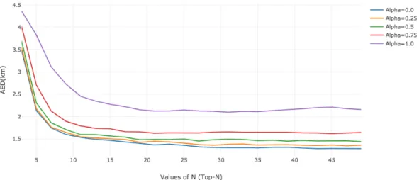
4.4 Distribution of the Average Error Distance (AED) in the Chicago dataset when considering values of N ∈ {3,5,7,9, ...,49} for the

Top-N most similar geotagged tweets. . . 73

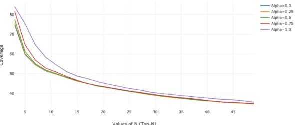
4.5 Distribution of the Coverage in the Chicago dataset when consid-ering values of N ∈ {3,5,7,9, ...,49} for the Top-N most similar

(21)

5.1 Distribution of average error distance (AED) for the Chicago dataset. The gure presents the distribution of our best performing learning to rank approach (L2Geo+MV@Top-13 using Query_Common) and the baseline (MV@Top-47). . . 97

5.2 (Chicago Dataset) Distribution of average error distance (AED) over the values of N ∈ {3,5,7,9,11, ...,49} for the Top-N

geo-tagged tweets considered by the majority voting algorithm. Bold line represents the best performing model (L2Geo using Query_-Common) . . . 98

5.3 (Chicago Dataset) Distribution of coverage (Coverage) over the values of N ∈ {3,5,7,9,11, ...,49}for the Top-N geotagged tweets

considered by the majority voting algorithm. Bold line represents the best performing model (L2Geo using Query_Common) . . . . 98

5.4 (New York Dataset) Distribution of average error distance (AED) over the values of N ∈ {3,5,7,9,11, ...,49} for the Top-N

geo-tagged tweets considered by the majority voting algorithm. Bold line represents the best performing model (L2Geo using Query_-Common) . . . 99

5.5 (New York Dataset) Distribution of coverage (Coverage) over the values of N ∈ {3,5,7,9,11, ...,49}for the Top-N geotagged tweets

considered by the majority voting algorithm. Bold line represents the best performing model (L2Geo using Query_Common) . . . . 99

6.1 Geographical distribution of trac crashes (N=886) in the city Chicago during the testing period (25th July to 1st August 2016). 112

6.2 Trac Incident Detection Pipeline. We integrate our ne-grained geolocalisation apporach to infer the geolocation of non-geotagged trac tweets. . . 119

6.3 Accuracy (y-axis) for 1 minute to 30 minutes after the incident (x-axis) for the trac incident-related geolocalised tweets using our ne-grained geolocalisation approaches. . . 123

(22)

6.4 Incident Detection Rate (y-axis) for 1 minute to 30 minutes after the incident (x-axis) for the trac incident-related geolocalised tweets using our ne-grained geolocalisation approaches. . . 124

6.5 Accuracy (y-axis) for 1 minute to 30 minutes after the incident (x-axis) for the trac incident-related geotagged tweets (Geotagged), and the expanded samples using tweets geolocalised using our ne-grained geolocalisation approaches. . . 125

6.6 Incident Detection Rate (y-axis) for 1 minute to 30 minutes af-ter the incident (x-axis) for the trac incident-related geotagged tweets (Geotagged), and the expanded samples using tweets geolo-calised using our ne-grained geolocalisation approaches. . . 126

(23)

Part I

(24)

Chapter 1

Introduction

1.1 Introduction

Social media services enable users to connect across geographical, political or eco-nomic borders. In particular, Twitter1 _{represents the most important microblog} service in the world with 336 million active users as of 20182_{. Twitter allows} users to share short messages instantaneously with the community discussing a wide range of topics. In particular, through its users' messages, Twitter provides a unique perspective of events occurring in the real world (Abbasi et al., 2012) with rst-hand reports of the people that are witnessing such events. Addition-ally, users posting from mobile devices have the option to attach geographical information to their messages in the form of GPS coordinates (longitude and lat-itude). These characteristics of Twitter have gained increasing popularity within several research communities, such as Computing Science and Social Science. Researchers in such communities aim to exploit Twitter data as a new source of time geotagged information for a broad range of applications, including real-time event detection (Atefeh and Khreich, 2015), topic detection (Hong et al.,

2012b), and disaster and emergency analysis (Ao et al., 2014; Imran et al., 2015;

McCreadie et al.,2016).

As location knowledge is critical for such applications, virtually all the analy-sis conducted in such tasks utilise geotagged Twitter data exclusively. However, since only 1% of messages in the Twitter stream contain geographical information

1_{https://twitter.com/}

(25)

(Graham et al.,2014), the available sample size for analysis is quite limited. Fur-thermore, Twitter users who publish geographical information have been found to be not representative of the broader Twitter population (Sloan and Morgan,

2015). This limitation is particularly crucial to transportation applications, where several new approaches have emerged to study transportation patterns, travel be-havior and detect trac incidents using Twitter data (Cui et al.,2014; D'Andrea et al., 2015; Gu et al., 2016; Kosala et al., 2012; Mai and Hranac, 2013; Schulz et al., 2013b; Steiger et al., 2014). Thus geolocating (or geolocalising) new non-geotagged tweets can increase the sample of non-geotagged data for these applications, which can lead to an improvement in their performance.

Earlier studies on the geolocalisation of tweets have limitations in the precision of the spatial resolution achieved; they are capable of geolocalise tweets at a coarse-grained level (i.e., country or city level) (Eisenstein et al.,2010a; Han and Cook,2013;Kinsella et al.,2011;Schulz et al.,2013a). Therefore, the accuracy of existing methods remains insucient for a wide range of applications that require highly accurate geolocated data. In this thesis, we aim to bridge this gap and investigate whether we can infer the geolocation of tweets at a ne-grained level (i.e., street or neighbourhood level). We advance the existing state-of-the-art further by developing novel ne-grained geolocalisation approaches, such that it is possible to infer the geolocation of tweets at a reasonable ne-grained level.

In particular, in this thesis, we aim to infer the most likely geolocation for a given tweet using its text as a source of evidence. It is important to note that, by doing this, we predict the geolocation encoded within the content of the tweet, which does not necessarily correlates with the geolocation where the user generated the tweet. For instance, when an event occurs, tweets describing such events can be generated by users that are physically at the location of the occurrence, or by users that are aware of such event but are physically located at another location. This issue is not relevant for the tasks we aim to assist with the methods developed in this thesis - i.e., trac incident detection or disaster and emergency analysis-, where the ultimate goal is to detect and geolocate events regardless of the geolocation where the user generated the tweet.

The essential argument made by this thesis is that the ne-grained geolocalisa-tion of tweets can be achieved by exploiting the characteristics of already available

(26)

individual nely-grained geotagged tweets. In particular, we exploit such relation to infer the geolocation of non-geotagged tweets based on their similarity to other geotagged tweets.

We address three main issues concerning the ne-grained geolocalisation of tweets and propose an evolution of techniques to tackle them. First, we investigate the limitations of existing tweet geolocalisation approaches when working at ne-grained levels. Mainly, these approaches follow the strategy of creating a virtual document to represent an area, which is generated by aggregating the texts of the geotagged tweets belonging to that area. We show that this strategy leads to a loss of important evidence and aects the geolocalisation at a ne-grained level. To alleviate such limitations, we use individual geotagged tweets instead of an aggregation of them, and propose a new approach for ne-grained geolocalisation based on a ranking of such individual geotagged tweets. Then, we return the location of the Top-1 geotagged tweet as the predicted location coordinates.

Second, we discuss the predictability of the location of tweets at a ne-grained level. We postulate that, in order to nd a ne-grained location for a given non-geotagged tweet, we should nd a correlation between its content similarity and geographical distance to other geotagged tweets. To this end, we propose a new approach that uses a majority voting algorithm to nd such a correlation by employing the geographical evidence encoded within the Top-N most similar geotagged tweets to a non-geotagged tweet.

Finally, we investigate the eects of the quality of the ranking of geotagged tweets on ne-grained geolocalisation. In particular, we propose a learning to rank approach to re-rank geotagged tweets based on their geographical proximity to a given non-geotagged tweet, and propose multiple features tailored for the ne-grained geolocalisation of tweets. This approach can improve the ranking of geotagged tweets and, therefore, lead to better ne-grained geolocalisation.

Additionally, this thesis investigates the applicability and generalisation of our ne-grained tweet geolocalisation approaches in a practical application related to the detection of trac incidents, which aims to use Twitter as a data-source for detecting trac incidents occurring in a city. Existing approaches to the task aim to detect an incident by identifying incident-related content in the geotagged tweets. Then, the predicted location of the incident is given by the location of the

(27)

incident-related geotagged tweets. We show how our ne-grained geolocalisation approaches are capable of inferring the geolocation of non-geotagged incident-related tweets and eectively predict the location of the incidents. Moreover, we show how trac incident detection is improved by adding new geolocalised incident-related tweets to the sample of already available geotagged tweets that is commonly used by existing trac incident detection approaches.

The remainder of this chapter presents the statement and contributions of this thesis, as well as a roadmap of its structure.

1.2 Thesis Statement

This thesis states that the geolocalisation of non-geotagged tweets at a ne-grained level1_{can be achieved by exploiting the characteristics of already available} individual nely-grained geotagged tweets. We assume a relationship between content similarity and geographical distance amongst tweets that are posted within an area. Thus, if two tweets are similar to each other, then they are likely to be posted within the same location. In order to validate our statement, we formulate the following four main hypotheses that will be explored in our three main contributions chapters. The rst three hypothesis relates to the ne-grained geolocalisation problem. Besides, the fourth hypothesis aims to validate the applicability and generalisation of our approaches.

• Hypothesis 1: By considering geotagged tweets individually we can

pre-serve the evidence lost when adapting previous approaches at a ne-grained level, and thus we can improve the performance of ne-grained geolocalisa-tion (Chapter 3).

• Hypothesis 2: The predictability of the geolocation of a tweet at a

ne-grained level is given by the correlation between its content similarity and geographical distance to nely-grained geotagged tweets (Chapter 4).

• Hypothesis 3: By improving the ranking of geotagged tweets with respect

to a given non-geotagged tweet, we can increase the number of similar and

(28)

geographically closer geotagged tweets, and thus we can obtain a higher number of ne-grained predictions (Chapter 5).

• Hypothesis 4: By geolocalising non-geotagged tweets we can obtain a

more representative sample of geotagged data and, therefore, improve the eectiveness of the trac incident detection task (Chapter 6).

1.3 Contributions

The key contributions of this thesis can be summarised as follows:

• An investigation into the performance issues of existing tweet

geolocalisa-tion approaches when applied to work at a ne-grained level.

• A novel ranking approach that alleviates state-of-the-art issues and enables

ne-grained geolocalisation of tweets.

• An study into what makes the geolocation of a tweet predictable at a

ne-grained level. We explore the relationship between content similarity and geographical distance to derive assumptions to improve the geolocalisation.

• A new model for ne-grained geolocalisation based on a weighted majority

voting that combines the geographical evidence of the most similar geo-tagged tweets.

• We demonstrate the eectiveness of the proposed geolocalisation approach

in the trac incident detection task. We expanded the sample of already available geotagged data and study the improvements in performance in detection rate.

1.4 Thesis Outline

In this thesis, we propose a geolocalisation approach for inferring the location of non-geotagged tweets at a ne-grained level. Initially, in the rst chapters, we focus on tackling the ne-grained geolocalisation problem. Next, we evaluate the eectiveness of the proposed approach in the context of a practical application

(29)

(i.e., trac incident detection). The remainder of this thesis is organised as fol-lows:

Part I: Introduction and Background

Chapter 2 introduces the concepts this thesis relies on. Firstly, we provide con-cepts from classical IR such as retrieval, indexing and approaches for weighting documents (including Vector Space Models and Probabilistic models) that we will utilise through the work of this thesis. Secondly, we provide a literature overview of previous research regarding the geolocalisation of Twitter data. This overview includes reviews of the approaches proposed to tackle the two main problems in the area: Twitter user and Tweet geolocalisation. Finally, we introduce the problem of ne-grained geolocalisation of non-geotagged tweets and motivate the limitations of previous research for tackling this task.

Part II: Fine-Grained Geolocalisation of Tweets

Chapter 3 investigates the limitations of previous tweet geolocalisation ap-proaches when working at ne-grained levels. We show that the strategy of existing approaches of aggregating geotagged tweets to represent a location leads to a loss of important evidence for ne-grained geolocalisation. To alleviate such limitations, we propose to avoid such aggregation and propose an approach for ne-grained geolocalisation based on a ranking approach of individual geotagged tweets. Finally, we experiment to demonstrate the eectiveness of our approach and provide insights to understand the drawbacks of existing state-of-the-art works.

Chapter 4 discusses the predictability of geolocation of tweets at a ne-grained level. We postulate that such predictability is given by a correlation between content similarity and geographical distance to other geotagged tweets. We ex-tend our ranking of individual geotagged tweets by adopting a weighted majority voting algorithm to exploit the geographical evidence encoded within the Top-N

(30)

geotagged tweet in the ranking.

Chapter 5 investigates the eects of the quality of the ranking on ne-grained ge-olocalisation. In particular, we propose a learning to rank approach that re-ranks individual geotagged tweets based on their geographical proximity to a given non-geotagged tweet. Moreover, we propose multiple features tailored for ne-grained geolocalisation of tweets and investigate the best performing combination of them. Part III: Applicability of The Fine-Grained Geolocalisation Approach Chapter 6 investigates the eectiveness of our proposed ne-grained geolocalisa-tion approaches when applied in a practical applicageolocalisa-tion. In particular, we study the eectiveness of geolocalised tweets in the trac incident detection task, which aims to detect real-time trac disruptions using messages posted in the Twitter stream. We geolocalise new non-geotagged incident-related tweets and demon-strate that, when comparing to a ground truth of real incidents, our approaches can eectively infer their location. Moreover, we show how the overall eective-ness of the trac incident detection task is improved when expanding the sample of incident-related geotagged tweets with new geolocalised incident-related tweets, compared to the performance when using geotagged tweets alone.

Part IV: Conclusions and Future Work

Chapter 7 provides conclusion remarks of the work undertaken in this thesis and discusses the new research questions that this thesis opens to the research community, and are worth to be investigated in the future.

1.5 Origin of The Material

The research material appeared in this thesis has been published in various journal and conference papers during the course of this PhD programme:

(31)

1. (Gonzalez Paule et al.,2017) On ne-grained geolocalisation of tweets. IC-TIR'17, pages 313-316.

2. (Gonzalez Paule et al.,2018b) On ne-grained geolocalisation of tweets and real-time trac incident detection. In Information Processing & Manage-ment.

3. (Gonzalez Paule et al., 2018a) Learning to Geolocalise Tweets at a Fine-Grained Level. CIKM'18, pages 1675-1678.

4. (Gonzalez Paule et al., 2019) Beyond geotagged tweets: exploring the ge-olocalisation of tweets for transportation applications. In Transportation Analytics in the Era of Big Data, Springer, pages 121.

In addition, the work undertaken during this PhD programme has lead to the publication of other research papers that have contributed to the elds of Geographical Sciences and Social Sciences. In particular:

5 (Thakuriah et al., 2016) "Sensing spatiotemporal patterns in urban areas: analytics and visualizations using the integrated multimedia city data plat-form." Built Environment 42.3, pages 415-429.

6 (Sun and Gonzalez Paule, 2017). "Spatial analysis of users-generated rat-ings of yelp venues." Open Geospatial Data, Software and Standards 2.1, pages 5.

(32)

Chapter 2

Background

and Related Work

2.1 Chapter Overview

In this chapter, we introduce the necessary concepts, denitions and methods that will be used later in this thesis. In particular, we provide essential background for understanding the methodologies used in PartII. Now we provide an overview of the content of this chapter.

Firstly, in Section2.2we introduce the eld of Information Retrieval (IR), that allows users to eciently and eectively search for relevant information within large collections of text documents by means of a query. Then, the documents are ranked by the estimated relevance with respect to the user's query. We start by describing the main components of an IR system and how text documents are processed and indexed. Lastly, we describe how relevant documents are retrieved using a retrieval model. Methods and techniques explained in this section will be used later in our experiments. Therefore, we formalise and describe in detail the state-of-the-art retrieval models that will be used in Part II of this thesis. However, while IR systems rank documents based on relevance to a given query, given the nature of our task (geolocalisation of a tweet), we aim to rank tweets based on their geographical proximity to a given tweet as a query. The behaviour of IR models in the context of this task will be explored in further experiments in this thesis.

Next, in Section2.3 we describe the challenges arisen when dealing with ter data in an IR system, which is the data source used through this thesis.

(33)

Twit-AND RELATED WORK 2.2 Information Retrieval Background ter messages have particular characteristics, they are short documents and are normally written in formal language. Because of this, state-of-the-art IR models, that were initially tailored to work with large text documents, under-perform when dealing with Twitter posts. For this reason, we introduce how the IR com-munity have tackled this issue and the best ways to store and process Twitter posts. These methods will be crucial for the experiments undertaken later in this thesis.

Finally, in Section2.4 we discuss related work regarding the geolocalisation of Twitter data. We introduce the eld and discuss the two main task tackled by the research community: Twitter user geolocalisation and tweet geolocalisation. Since this thesis aims to investigate the tweet geolocalisation task, we then describe the main approaches that researchers have proposed in the past to address the problem. Lastly, we motivate the problem of inferring the geolocalisation of tweets at a ne-grained level and motivate the work in this thesis.

2.2 Information Retrieval Background

The eld of information retrieval (IR) deals with the representation, storage, organisation of and access to information items (Baeza-Yates et al., 1999). The discipline was developed to eciently and eectively access information contained in large collections of text documents written in natural language. The process of IR can be summarised as follows. Firstly, a user with an information need introduces a text query using natural language into an IR system that stores a collection of text documents. The collection is stored in the IR system using a data structure called index, which allows ecient access to the items. Secondly, the IR system processes the query and assigns to each document a score that represents an estimation of how the document matches the information need ex-pressed by the user in the query, this is called relevance. Finally, the system presents the documents as a ranked list ordered by their level of estimated rele-vance.

The concept of relevance is key in IR. A depth of understanding of the decision making processes occurring in the human brain is needed to understand user's information need fully, and users normally express this poorly in their queries.

(34)

AND RELATED WORK 2.2 Information Retrieval Background Instead, the IR system usually estimates relevance by calculating the similarities between the content of the query and the content of the documents. This is the goal of the retrieval model, which is the core of any IR system. In this thesis, we utilise retrieval models in order to assess the similarities between tweets for geolocalisation. Thus, in this chapter, we introduce a general background of the Information Retrieval (IR) concepts required to understand the topics explored in this thesis. The rest of the chapter is organised as follows: Section2.2.1introduces eective indexing strategies followed by retrieval systems. Section 2.2.2discusses the principles and formalisation of retrieval models. Section 2.2.3 details the Learning to Rank framework that uses machine learning for information retrieval.

2.2.1 Indexing

In order to eectively search for relevant items within a collection of documents, retrieval systems perform a process named indexing. During indexing, rst text documents are transformed into a bag-of-words representation and stored into an ecient data structure called index. In this section, we rst describe how docu-ments are transformed in Section2.2.1.1and discuss how the index is constructed to eciently search the documents in Section 2.2.1.2.

2.2.1.1 Document Transformation

The rst stage of the indexing process is transforming documents into a bag-of-words representation in order to store them into the index. The rst step of document transformation is called tokenisation. In this process, documents are rst decomposed into terms by identifying the boundaries (or separator) between tokens (or terms). All terms are lowercased, and all the punctuation is removed at this stage. For instance, given the following document taken fromCarroll(2011):

Begin at the beginning, the King said gravely, and go on till you come to the end: then stop.

after tokenisation, the above document is transformed into:

begin at the beginning the king said gravely and go on till you come to the end then stop

(35)

AND RELATED WORK 2.2 Information Retrieval Background According to Luhn (1957), the discriminative power of a term is normally distributed with respect to the rank of its frequency in a collection. Moreover, common terms (e.g., the) will occur in almost all documents. Such are typically known as stopwords, and their informativeness in terms of the relevance of a document is null. For this reason, stopwords are removed from the text.

In order to determine which terms are considered for removal, a list of pre-compiled stopwords is used. Several stopwords lists have been proposed in the literature (Van Rijsbergen,1979), and typically consisting of prepositions, articles and conjunctions. Also, other terms can be extracted automatically by determin-ing the most frequent and less informative terms within a collection (Lo et al.,

2005). After stopword removal, the example document above is reduced to the following:

begin beginning king said gravely you come end then stop

Usually, the term specied in a query by the user is not in the same syntactic variation as it is present in relevant documents (Baeza-Yates et al., 1999), which prevents perfect matching between the query and the document. For example, I am living in Scotland is a dierent syntactical variation than I have lived in Scotland. To overcome this issue, terms are transformed and reduced to their stem using a Stemming algorithm. For example, the words shing, shed, and sher are transformed to the root word, sh. The rst stemming algorithm was proposed byLovins(1968), which then inuenced the Porter Stemming algorithm (Porter,1980), which is the most popular. After applying stemming the example document is reduced to the following:

begin begin king said grave you come end then stop

Finally, the resulting text is transformed into a bag-of-words representation by counting the number of times a term occurs in the document. This set of terms in a document with their frequencies is the nal representation of a document-terms list that is stored in the index data structured. The nal document-terms list for the example document is shown in Table 2.1.

(36)

AND RELATED WORK 2.2 Information Retrieval Background Table 2.1: A bag-of-words representation of a document.

Document Term Frequency begin 2 king 1 said 1 grave 1 you 1 come 1 end 1 then 1 stop 1

2.2.1.2 Index Data Structures

After each document of a collection is transformed into a bag-of-words represen-tation they are stored into the index as a document-terms list. However, in order to score documents with respect to the terms in a query, the retrieval system is forced to iterate through all of the document-terms list. This has a cost ofO(N) time complexity, where N is the total number of documents in the collection, and this is not scalable to handle large collections. In order to eciently score documents, an alternative data structure was proposed, called inverted index (Van Rijsbergen, 1979). This data structure transposes the document-terms list into a term-documents list. This way, the system only scores the subset of doc-uments (Dq) that contain the terms of the query, which reduce time complexity to O(Dp).

After the collection has been indexed, documents are ready for being ranked in response to a query based on a probability score given by a retrieval model. In the next section, we describe the traditional approaches for scoring and ranking documents.

2.2.2 Retrieval Models

Given an indexed collection of documents, the primary goal of an IR system is to rank documents based on their probability of meeting the information need of the user, which is expressed as a query. In order to fully understand how humans

(37)

AND RELATED WORK 2.2 Information Retrieval Background judge relevance with respect to their information needs, it would be necessary to understand the cognitive process of decision making that occurs in the human brain. Instead, IR researchers have developed theoretical assumptions that aim to capture how documents match information need given a query. These theoretical assumptions are then formalised into a mathematical model, named retrieval model. In the rest of this chapter, we detail the most well-known approaches for retrieval, including the models that we will utilise in this thesis.

Fundamentally, a retrieval model estimates relevance as a quantication of the similarities between a document and a query. Thus, IR models assume that the most similar documents to a given query are considered to be the most relevant to the user information needs. This is typically done by a weighting the model using statistical features of the document, the query and the collection. For this reason, retrieval models are also known as document weighting models or IR weighting models.

2.2.2.1 Boolean Model

One of the rst models for document retrieval is the Boolean Model (Van Ri-jsbergen, 1979). The boolean model is based on set theory and boolean logic. Documents are considered as sets of terms with a binary weight to represent whether they occur in the document or not. Moreover, the boolean model has no information regarding term importance in the query, document or collection. Queries are composed as a combination of terms and boolean logic operators such as AND, NOT and OR, which state whether the presence of a term is required or excluded in the document. Due to the boolean nature of the query, a boolean relevance score is assigned to the documents; either TRUE or FALSE. Hence, the Boolean Model is also named as exact-match retrieval since only documents that match the query are retrieved. Because a binary relevance score is assigned to the documents, there is no ranking per se and documents are often ordered by other metadata information such as creation date or author.

The main drawback of the Boolean Model is that there is no partial matching to the query, i.e. the model does not provide a degree of relevance. This has an impact on eectiveness which mainly depends on how well the users formulate the queries. Moreover, query formulation based on boolean logic is unnatural and

(38)

AND RELATED WORK 2.2 Information Retrieval Background presents a dicult way for the user to express their information needs (Van Ri-jsbergen, 1979). Despite these disadvantages, the boolean model is utilised in several applications, such as patent search (Joho et al., 2010), due to its e-ciency.

2.2.2.2 Vector Space Model

The Vector Space Model (VSM) was the focus of IR research in the 1970s and was proposed to overcome the limitations of the Boolean model. The main new advantages of the VSM is to allow partial matching of the query and incorporate estimations about the relevance of the documents (Dillon, 1983; Salton et al.,

1975). Therefore, the resulting list of matched documents can be ranked according to their degree of relevance to a query. In order to do that, the VSM uses a n -dimensional space of Euclidean geometry, where n is the number of terms in the index (or collection), and each dimension represents the weight of the term.

Then, in the VSM, documents and queries are represented as vectors in the above mentioned n-dimensional Euclidean space. In particular, a document di is represented by a vector of terms _V~₍_d_i_{) = (}_d_i,₁_{, d}_i,₂_{, ..., d}_i,n₎_{, where} _d_i,j _{is the} weight of the j-th term in the document. Likewise, a query q is represented as a vector of terms _V~₍_q_{) = (}_q₁_{, q}₂_{, ..., q}_n₎_{, where} _q_j _{is the weight of the} _j_{-th term in} the query. In the most simple form of the VSM, the weight of each term is the raw count or term frequency (tf), which term provides a measure of the importance of the term in a document. Nevertheless, other approaches for term weighting has been explored. These approaches incorporate A new statistic named Inverse Document Frequency (idf) that was proposed by Sparck Jones (1972). The idf statistic calculates the number of documents over the entire collection where the term occurs at least once, and reects the importance of a term in the entire collection. Finally, the TF-IDF weighting scheme is the most commonly used for weighting the vectors, thus the tf-idf of the term w in a document di can be dened as:

tfi,w×idfw =tfi,w·log N dfw

(39)

AND RELATED WORK 2.2 Information Retrieval Background whereN is the number of documents in the collection,tfi,w is the term frequency of the term w in the document di, and dfw is the number of documents in the collection where w appears at least once.

Once the document and the query vectors are constructed, the Euclidean dis-tance can be used to compute the level of similarity (as an estimation of their relevance). However, instead of calculating the distance (or dissimilarity) a simi-larity measure is commonly employed to predict relevance. Therefore, documents with the highest scores are considered the most similar and, therefore, should be ranked at the top of the list.

Several similarity measures have been proposed in the literature (Van Rijsber-gen,1979). The most popular is known as the cosine similarity, which we utilise in this thesis. The cosine similarity computes the cosine of the angle θ between two vectors. Thus, the similarity between the document di and the query q is calculated as the cosine of the angle θ between the document vector V~(di) and the query vector _V~₍_q₎ _{dened as:}

similarity(di, q) =cosineθdi,q = ~ V(q)·V~(di) |V~(q)| · |V~(di)| (2.2) 2.2.2.3 Probabilistic Models: BM25

Previous retrieval models assessed relevance in dierent ways. The Boolean model determined relevance by a binary decision of the existence of the query terms in the document. Then, in the Vector Space Model relevance is determined by the cosine similarity of two weighted vectors in a Euclidean space representing the document and the query. However, relevance can also be quantied as a value that measures the level of uncertainty that the content of a document is relevant to the user's information need. This is the basic principle of Probabilistic Retrieval Models, that are rooted by the Probability Ranking Principle (PRP) (Cooper,

1971; Robertson, 1977) and is based on the foundations of probability theory. The PRP is stated as:

If a reference retrieval system's response to each request is ranking of the documents in the collections in order of decreasing probability of relevance to the

(40)

AND RELATED WORK 2.2 Information Retrieval Background user who submitted the request, where the probabilities are estimated as accurately as possible on the basis whatever data have been made available of the

system for this purpose, the overall eectiveness of the system to its user will be the best that is obtainable on the basis of those data.

The PRP assumes that the probability of relevance of a document to a query is independent of other documents. Based on this assumption, and applying the Bayes Theorem, a new probabilistic weighting model for retrieval can be derived. The most notable model is the Okapi BM25 (Robertson et al., 1995), which will be used in this thesis. In the Okapi BM25 the probability of a document d to be relevant to a given query q is dened as follows:

P(rel|d, q)∝X t∈q log N −dfi+ 0.5 dfi+ 0.5 · (k1+ 1)·tfi k1((1−b) +b_avgdldl ) +tfi

where tfi represents the frequency of the term in the document, dfi is the docu-ment frequency of the term, and docudocu-ment length is represented asdl. Document length is normalised by dividing the length of the document by the average docu-ment length of the collectionavgdl. The model is tuned using two parameters;k1 and b. By adjustingk1we control the inuence of term frequency tfi in the nal score, whereas adjusting b varies the inuence of document length normalisation

dl

avgdl.

2.2.2.4 Language Modelling

Statistical Language modelling has been applied to predict the next term given an observed sequence of terms. Thus, a language model is a probability distri-bution over sequences of terms (Manning et al., 1999). In the context of IR, a language model represents, in essence, the probability of observing a term in a document. Language modelling was introduced as a ranking approach in the late 1990s (Berger and Laerty,2017; Hiemstra, 1998;Miller et al.,1999b;Ponte and Croft, 1998). From a statistical perspective, language models (LM) are funda-mentally dierent to probabilistic models (PM) in Section 2.2.2.3. Probabilistic models determine relevance for a document given a query, whereas language mod-els calculate the probability of a query of being generated by a document.

(41)

AND RELATED WORK 2.2 Information Retrieval Background The Language Modelling (LM) approach attempts to model the process of generating of a query (Ponte and Croft, 1998) given a document. The approach assumes that a queryqis generated by a probabilistic model based on observations of terms in a document d. Thus, we aim to calculate the conditional probability P(d/q). By applying Bayes' rule we obtain:

P(d|q) = p(q|d)p(d)

p(q) ∝p(q|d)p(d) (2.3) where p(d) is the prior belief that the document is relevant to any query, and p(q|d)is the query likelihood given the document. Note thatp(q) is ignored as it is the same for every document in the collection, and therefore does not aect the ranking of the documents in response to a query. The priorp(d)is mostly assumed to be uniformly distributed (Berger and Laerty,2017;Hiemstra,1998;Ponte and Croft, 1998), but many alternative priors has been also investigated in the past (Miller et al., 1999a). In this thesis, we assume a uniform prior distribution. After this simplication, the model is reduced to the task of estimating p(q|d), the probability of observing the query q given the document d. Thus, using a multinominal unigram language model, the probability of generating the query terms using document d is formalised as:

ScoreQLM(q, d) = p(q|d)∝

Y

t∈q

p(t|θd)tft,q (2.4)

where p(t|d) is the probability of observing a term t of the query given the lan-guage modelθdfor documentd, andtft,q denotes the term frequency of the termt in the queryq. Note that, in order to calculatep(t|θd), a sparsity problem appears as a term t in a query may not be present in the document d. This is called the zero probability problem. To tackle the problem of zero probabilities for unseen terms, the language model of the document is complemented with the collection model, which has knowledge of any term in the entire collection. This technique is known as smoothing, and various strategies for doing so have been proposed in the literature (Zhai and Laerty, 2017): Jelinek-Mercer, Dirichlet and Absolute discounting.

(42)

AND RELATED WORK 2.2 Information Retrieval Background In this thesis, we will deal with Twitter data as we explain later in Section

2.3. Experiments realised by Zhai and Laerty (2017) showed that Dirichlet smoothing performs the best when using title queries, that are short queries containing mostly two or three keywords. This is in line with the average query length in Twitter search reported byTeevan et al. (2011) (1.64 words per query). Additionally, language models with Dirichlet smoothing have been used as the baseline retrieval models for the 2013 and 2014 instances of the microblog search tracks (Lin and Efron,2013; Lin et al., 2014) that we introduce in detail later in Section 2.3. For these reasons, in our experiments, we apply the language model approach that applies Dirichlet smoothing, which we will describe next.

Dirichlet Smoothing. For any language model, the general form for smooth-ing is given by:

P(t|d) =

(

ps(t|d) if term t is seen, αdp(t|C) otherwise

(2.5) where ps(t|d) is the probability of a term in the document d, αp(t|C) is the probability of a term in the entire collectionCandαdis a coecient that controls the probability assigned to unseen terms. In the Language Model with Dirichlet smoothing, the prior distribution of terms in the collection is given by a Dirichlet distribution with parameters (µp(t1|C), µp(t2|C), ..., µp(tn|C)). Thus, the model is given by:

p(t|d) = tf_Pt,d+µp(t|C) ttfw,d+µ

(2.6) where tft,d is the frequency of the term t in the document d, and µ is the con-trolling coecient for the smoothing.

2.2.2.5 Divergence From Randomness

Divergence From Randomness (DFR) is a probabilistic approach that works under the assumption that the more the content of a document diverges from a random distribution, the more informative the document is Amati(2003). Therefore, the

(43)

AND RELATED WORK 2.2 Information Retrieval Background most informative terms are distributed over an elite set of documents, whereas the non-informative terms are randomly distributed over the entire collection (Bookstein and Swanson,1974;Damerau,1965;Harter,1975a,b). The underlying hypothesis of DFR models is:

The informative content of a term can be measured by examining how much the term frequency distribution departs from [...] the distribution described by a

random process (Amati, 2003)

Thus, to compute the importance of a given termtin a document d, the DFR models calculate the distribution of its term frequency tf in the documents, and compute its divergence from a distribution generated through a random process. The standard DFR model, given a query q and a document d, is dened as:

ScoreDF R(d, q) =

X

t∈q

wt,qwt,d (2.7)

where wt,q is the normalised frequency of term t in the queryq, given by: wt,q =

tft,q maxti∈qtfti,q

(2.8) and wt,d is the weight of a term t in a document d is given by:

wt,d =inf1inf2 (2.9)

The frequency of the term in the document wt,d is composed by inf1 =

−log₂p1(t|C) and inf2 = 1−p2(t|d), which denes the informativeness of the

term t in the entire collection C and in a document d that contains the term, respectively.

The component p1(t|C) is named the basic randomness model of the

(44)

AND RELATED WORK 2.2 Information Retrieval Background the following1 ₍_Amati_,₂₀₀₃_{): divergence approximation of the binomial (}_D_), ap-proximation of the binomial (P), Bose-einstein distribution (Be), geometric ap-proximation of the Bose-einstein (G), inverse document frequency model (I(n)), inverse term-frequency model (I(F)), and inverse expected document frequency model (I(ne)).

On the other hand, the p2(t|d) component denes the information gain of

observing the termtin the documentd. This can be computed using two models: Laplace (L) model: L= 1 tft,d+ 1 (2.10) and the ratio of two Bernoulli's process (B):

B = F dft,c(tft,d+ 1) (2.11) However, a third component is needed for DFR models. Because the amount of information in a document is in proportion to its length, a document length normalisation is needed, called N ormalisation2, as dened bellow:

tfn=tf ·log 1 +c·avgdl dl (2.12) In this thesis, we experiment with dierent combinations of the components mentioned above, which congure dierent DFR models. We now briey intro-duce them as described in (Amati, 2003):

InB2: Inverse Document Frequent model with Bernoulli after-eect and normal-isation 2. wt,d= F + 1 nt·(tf n+ 1) tf n·log₂ N + 1 nt+ 0.5 (2.13)

1_{As described in the Terrier IR platform (}_{Ounis et al.}_,₂₀₀₆_{) (}_{http://terrier.org/docs/} v3.5/dfr_description.html)

(45)

AND RELATED WORK 2.2 Information Retrieval Background IneB2: Inverse Expected Document Frequent model with Bernoulli after-eect and normalisation 2. wt,d = F + 1 nt·(tf n+ 1) tf n·log₂ N + 1 ne+ 0.5 (2.14) IFB2: Inverse Term Frequency model with Bernoulli after-eect and normalisa-tion 2. wt,d= F + 1 nt·(tf n+ 1) tf n·log₂ N + 1 F + 0.5 (2.15) InL2: Inverse Document Frequency model with Laplace after-eect and normal-isation 2. wt,d = 1 tf n+ 1 tf n·log2 N + 1 nt+ 0.5 (2.16) PL2: Poisson model with Laplace after-eect and normalisation 2.

wt,d= 1 tf n+ 1 tf n·log2 tf n λ + (λ−tf n)·log2e+ 0.5·log2(2π·tf n) with λ= F N and F N (2.17)

wheretf is the within-document frequency oftind,ntis the document frequency of t, F is the term frequency of t in the whole collection, N is the number of document in the whole collection, ne is the number of expected documents containing the term according to the binomial law (See Amati (2003); Section 4.5.2).

2.2.3 Learning to Rank

The ranking approaches described in previous sections aim to capture the rele-vance of a document for a given query. However, such models can be eective in specic search scenarios, but it is improbable that they can also be eective in

(46)

AND RELATED WORK 2.2 Information Retrieval Background all search scenarios Zhai and Fang(2013). This issue is particularly true for Web retrieval, due to the diversity in size and content of web pages and the variability and complexity of the information needs of the users that search the web (Liu et al.,2009). However, any single of such models can capture dierent aspects of the relevance of a document. Thus, by combining them as multiple features in a machine-learned ranking function, we can potentially provide eective results in multiple search scenarios. This is the aim of Learning To Rank (L2R) approaches. In the basic form of L2R approaches, features are extracted from a set of ranked documents to a given query to train a ranking function. This function is then applied to re-rank unseen document rankings and increase the desire ranking criteria (i.e., relevance in web retrieval) at the top documents in the list. Figure

2.1 present the general framework of learning to rank. As dened by (Liu et al.,

2009), in order to train the ranking function the learning to rank approach uses an initial sample of ranked documents with respect to a query, called training set. This sample of query-document pairs should have high-recall and should have many relevant documents (Macdonald et al., 2013).

Figure 2.1: Learning to Rank Framework (Liu et al., 2009).

(47)

litera-AND RELATED WORK 2.3 Information Retrieval for Twitter ture and can be categorised in three groups based on the number of documents that are taken into account for learning: point-wise approaches (Breiman, 2001;

Friedman,2001), pair-wise approaches (Burges et al.,2007; Wu et al., 2010) and list-wise approaches (Metzler and Croft, 2007; Xu and Li, 2007). Point-wise approaches consider each document in the sample ranking independently, pair-wise approaches consider pairs of documents and list-pair-wise approaches optimise an information retrieval measure and consider the entire ranking list at one time. Prior works have shown that list-wise approaches are the most eective (Liu et al.,

2009). However, this performance has not been investigated in the specic task of this work (tweet geolocalisation). In Chapter 5, we experiment with several types of L2R approaches and identify the best performing ones on our task.

2.3 Information Retrieval for Twitter

State-of-the-art Information Retrieval (IR) models are mainly tailored to provide a relevance estimation score to large text documents. The most common applica-tion of IR models is the search of web documents (Arasu et al., 2001), where the issues of IR models to work with the specic characteristics of web pages have been widely studied (Croft et al., 2010). However, with the appearance of Twit-ter, it also appeared the necessity of searching for information in Twitter posts. The task of information retrieval in the context of Twitter, where users issues textual queries to a search engine to nd relevant previously published tweets, is named Microblog Retrieval in the literature.

Due to the social characteristics of the Twitter content, the way how and why users search in Twitter diers from how users search the Web (Teevan et al.,

2011). Users' queries in Twitter search are shorter and are more repetitive to track specic results about social events. On the other hand, Web queries are more changing, and users develop more queries in order to nd more information about a topic.

In this section, we rst discuss the specic structural characteristics of Twitter documents and how they are preprocessed and indexed into the retrieval system. Next, we discuss recent research on the applicability of IR models in the context of a microblog search task.

(48)

AND RELATED WORK 2.3 Information Retrieval for Twitter