Moisture insensitive prediction of soil properties from VNIR reflectance spectra based on external parameter orthogonalization

(1)

Moisture insensitive prediction of soil properties from VNIR re

ﬂ

ectance

spectra based on external parameter orthogonalization

Nuwan K. Wijewardane

a

, Yufeng Ge

a,

⁎

, Cristine L.S. Morgan

b

a

Department of Biological Systems Engineering, University of Nebraska—Lincoln, Lincoln, NE 68583, USA b_{Department of Soil and Crop Sciences, Texas A&M University, MS2474 TAMU, College Station, TX 77843-2474, USA}

a b s t r a c t

a r t i c l e i n f o

Article history:

Received 11 December 2015 Accepted 14 December 2015 Available online 8 January 2016

Moisture is the single most important factor that affects soil reflectance spectra, particularly forfield applications. Interest in using soil VNIR spectral libraries, which are commonly based on dry ground soils, to predict soils in the intactfield-moist condition (in situ VNIR) is growing. External parameter orthogonalization (EPO) has been pro-posed as a useful method that links dry ground VNIR models tofield moist scans. The goal of this study is to test EPO on a wider set of soil properties and four different modeling techniques, namely, Partial Least Squares Re-gression (PLS), Artificial Neural Network (ANN), Random Forest (RF), and Support Vector Machine (SVM). We selected and scanned 352 archived soil samples from Nebraska, USA, among which 185 samples were used to de-velop dry ground models and the remaining 167 samples were rewetted to eight different moisture levels for EPO development and testing. Two methods to determine optimum number of EPO components, model-coupled cross validation (Model-Coupled-CV) and Wilk'sΛwere also compared. The results showed that EPO minimized the variability of soil spectra induced by moisture. Results suggest a preference for the Wilk'sΛmethod over Model-Coupled-CV for determining the number of EPO componentsg, as it produced smoother transformed spectra and more parsimonious models. Among the eight soil properties tested, EPO caused significant ments for soil Organic Carbon (OC), Inorganic Carbon (IC), and Total Carbon (TC) prediction, marginal improve-ment for sand and clay, and no improveimprove-ment for pH, Mehlich-3 Phosphorus, and Cation Exchange Capacity. The failed EPO for the latter three properties is attributable to the poor initial dry-ground models that EPO was built upon. For OC, IC, and TC, EPO coupled effectively with all four modeling methods, with ANN and SVM outperforming the other two slightly. This addsflexibility to the implementation of EPO in predictingfield moist soils. As there are increasing demands of spatially-explicit soil data in many disciplines, EPO would be an important essential part for the future in situ VNIR based proximal soil sensing technology.

Chemometric modeling

External parameter orthogonalization Soil carbon

Soil moisture VNIR

1. Introduction

Visible and near infrared re_ﬂectance spectroscopy (VNIR) is widely used as a rapid and cost effective method to quantitatively infer soil properties (Chang et al., 2001; Stenberg, 2010; Viscarra Rossel et al., 2006). Numerous studies have shown VNIR soil spectra to successfully predict a wide array of soil properties including soil carbon (Brown et al., 2006; Minasny et al., 2011; Nocita et al., 2013; Sarkhot et al., 2011), texture (Brown et al., 2006; Sørensen and Dalsgaard, 2005; Waiser et al., 2007), moisture (Ben-Dor et al., 2008; Mouazen et al., 2005; Zhu et al., 2010), and plant macro- and micro-nutrients (Ge et al., 2007; Shepherd and Walsh, 2002).

For a long time, there has been interest in the soil community to develop large soil spectral libraries (Brown et al., 2006; Shepherd and Walsh, 2002). Legacy (or archive) soil samples with partial or full char-acterization are available all over the world. This makes the establish-ment of large spectral libraries a feasible task. One great potential of soil spectral libraries is that they can be used for rapid soil characteriza-tion in theﬁeld.

While conceptually attractive, a primary challenge for using soil spectral libraries infield applications is the wide range of soil moisture that will be encountered. Spectral libraries are most likely constructed from dry and ground soils; butfield samples will be in quite different conditions in terms of moisture, small-scale heterogeneity, and temper-ature. Among these three factors, moisture has the most pronounced ef-fects on VNIR spectra (Bricklemyer and Brown, 2010; Kuang and Mouazen, 2013; Minasny et al., 2009; Sudduth and Hummel, 1993).The decrease of VNIR model performance, when dealing with field moist soil samples, is also documented in the literature (Bricklemyer and Brown, 2010; Minasny et al., 2009). Several authors ⁎ Corresponding author at: Department of Biological Systems Engineering, 209 Chase

Hall, East Campus, University of Nebraska—Lincoln, Lincoln, NE 68583, USA. E-mail addresses:[email protected](Y. Ge),[email protected](C.L.S. Morgan).

http://dx.doi.org/10.1016/j.geoderma.2015.12.014

0016-7061/© 2015 The Authors. Published by Elsevier B.V. This is an open access article under the CC BY-NC-ND license (http://creativecommons.org/licenses/by-nc-nd/4.0/). Contents lists available atScienceDirect

Geoderma

(2)

used VNIR spectra of intact soils and demonstrated successful prediction of intact soils (Gomez et al., 2008; Morgan et al., 2009; Waiser et al., 2007). But it is neither practical nor economical to develop both_ﬁeld moist spectral libraries and dry ground libraries due to the large number ofﬁeld samples needed.

External parameter orthogonalization (EPO) has recently emerged as a promising method to remove (or minimize) the effect of soil mois-ture on VNIR spectra (Roger et al., 2003). EPO decomposes a spectrum into two components: a useful component that has a direct relationship with the response variable, and a parasitic component that is from an external influence. By removing the parasitic component through or-thogonal transformation of spectra, the calibrated spectral model can be less sensitive to the external influence (soil moisture in our case) and more accurate when applied tofield moist soils.

The usefulness of EPO in soil spectra wasﬁrst demonstrated by

Minasny et al. (2011). The authors used 391 soil samples collected from New South Wales, Australia and createdﬁve different moisture levels under the laboratory condition. Scans of 100 samples were used for EPO development, 271 for model calibration and the remaining 20 for testing. The results showed that EPO successfully removed the mois-ture effect from soil VNIR spectra and improved the prediction accuracy of soil Organic C (OC). In addition they suggested using more than 100 samples for model calibration and 60 samples for the EPO development.

Ge et al. (2014)expanded the study of EPO to clay content and soil OC. They used both rewetted samples in the lab andﬁeld moist scans for EPO development and testing. All samples were collected from Texas, USA; and model calibration was done using Texas Soil Spectral Li-brary comprising more than 2000 samples. They showed that EPO from theﬁeld moist scans yielded large improvement in clay prediction. More recently, EPO was also tested for soils in China (Ji et al., 2015) and Brazil (Ackerson et al., 2015), both with positive results.

Previous research tested the validity of EPO in a narrow sense: they focused on the modeling of soil OC and clay, and PLS was the only modeling technique considered. In addition, all previous studies used the PLS-CV (Partial Least Squares—Cross Validation) method for deter-mining the optimal number of EPO components. In Roger et al. (2003), an alternative method, known as Wilk'sΛ, was also suggested for this purpose. As there are increasing demands for spatially explicit soil data at high spatial and temporal resolutions in many disciplines, in situ soil sensors based on VNIR will play a very important role to meet these demands at sufﬁcient accuracy and throughput. EPO will be-come an essential part of the in situ VNIR soil sensing system.

Our long term goal is to use VNIR libraries for inﬁeld soil characteriza-tion. In this study we want to further test the usefulness of EPO with the following two objectives: (1) test EPO on a wider set of soil attributes be-yond soil OC and clay, and (2) test the effectiveness of EPO when coupled with other nonlinear modeling techniques including Artiﬁcial Neural Net-work, Random Forest and Support Vector Machine. With the second ob-jective, we also compare the model-coupled-CV and Wilk'sΛmethods to determine the optimal number of EPO components.

2. Material and methods

2.1. Soil samples and dataset description

Soil samples used in this study were selected from the soil archive maintained by Kellogg Soil Survey Laboratory of USDA-NRCS. Samples in the archive are stored in air dried and ground (b2.0 mm) condition. The following criteria were used for sample selection from the archive. First, the samples are originated from Nebraska, USA. Second, the samples had the full characterization of eight chemical and physical properties: OC, Inorganic Carbon (IC), Total Carbon (TC), sand, clay, 1:1 water pH, Mehlich-3 Phosphorus (P), and Cation Exchange Capacity (CEC). Since OC is an emphasis property of this study, the third criterion involved the selection of samples representing the full range of OC in the archive through a 20-stratum stratiﬁed random sampling. As a result, a total of

352 samples were selected and used in this study. These samples were further divided into three non-overlapping subsets. They were described as follows, and similar notations as inRoger et al. (2003)are used.

Dry ground set (S0₎_—_{This set consisted of 185 samples to develop} dry ground multivariate models for different soil properties. Samples in this set were scanned once in dry ground condition.

EPO development set (S1₎_—_{This set consisted of 100 samples for} EPO development. Each sample in this set was scanned nine times: one scan in dry ground condition and eight scans at eight moisture levels (900 scans in total). A detailed description of soil rewetting proce-dure is in the next section.

Testing set (S2)—This set consisted of 67 samples for independent EPO validation. The samples in this set were also scanned nine times and in the same moisture condition asS1_{(603 scans in total).}

The summary statistics of soil properties in the three different sets are given inTable 1. Median and Interquartile Range (IQR) are present-ed instead of mean and standard deviation, because all properties ex-hibited non-normal distribution.

2.2. Rewetting procedure and VNIR scanning

Sample rewetting (n= 167) was carried out in 4 batches, where batch 1 had 35 soil samples; batch 2 had 46 soil samples; batch 3 had 46 soil samples; and batch 4 had 40 soil samples for easy handling dur-ing the experiment. Approximately 10 g of each sample in batch 1 were placed in petri dishes and scanned in the air dried conditionﬁrst. A known amount of deionized water was then added to each sample to achieve a moisture content of ~33% (dry basis, gravimetric). Petri dishes were covered with glass lids to avoid moisture loss to the outside and

Table 1

Summary statistics of the soil properties in three different subsets (S0 ,S1 , andS2 ) in this study. Soil property S0 _S1 _S2 No. of samples (n) 185 100 67 No. of scans (N) 185 900 603 Organic C (%) Min 0.0 0.1 0.0 Median 0.8 1.4 1.1 Max 6.2 6.5 5.7 IQR⁎ 1.2 1.3 1.5 Inorganic C (%) Min 0.0 0.0 0.0 Median 0.1 0.1 0.1 Max 3.8 1.9 3.9 IQR 0.3 0.2 0.8 Total C (%) Min 0.1 0.1 0.2 Median 1.2 1.5 1.5 Max 6.4 6.5 6.4 IQR 1.3 1.4 1.4 Sand (%) Min 0.2 0.5 0.9 Median 8.9 5.4 8.2 Max 99.2 98.4 96.5 IQR 34.8 23.3 28.6 Clay (%) Min 0.3 1.3 1.3 Median 30.0 28.5 29.3 Max 74.0 67.6 48.2 IQR 18.9 10.8 11.2 pH Min 4.4 4.7 5.2 Median 7.8 6.4 7.1 Max 10.1 8.4 8.6 IQR 0.8 1.5 1.6 P (mg kg−1 ) Min 0.2 0.0 0.0 Median 30.7 24.9 14.7 Max 244.2 162.4 195.7 IQR 52.7 40.2 42.9 CEC (cmol + kg−1 ) Min 1.7 1.4 1.9 Median 21.8 21.5 21.4 Max 51.8 47.1 43.5 IQR 12.4 7.9 6.9

⁎ IQR is Interquartile Range; CEC is Cation Exchange Capacity; and P is Mehlich-3 Phosphorous.

(3)

facilitate uniform moisture distribution within samples. After ~24 h, the petri dishes were weighed and then scanned to obtain theﬁrst set of moist scans. The lids were then kept open to enhance evaporation of water with continuous monitoring of moisture content. When samples reached the next desired moisture level, petri dishes were again covered with lids for 24 h (for moisture homogenization within samples) followed by scanning and weighing for the second moisture level. This step was repeated to obtain scans at eight different moisture levels. This procedure was applied to other batches with the exception that 15 g of soil were used in subsequent batches to better control moisture evaporation. Care was given to maintain the intended moisture levels to resemble theﬁrst batch. The average moisture levels for all the batches were 33, 29, 25, 21, 17, 13, 10 and 8% by weight; and all moisture con-tents were calculated as dry basis adjusted with the ADOD (Air Dried to Oven Dried weight) values for each sample. For the two rewetting sets (S1_and_S2_{), ADOD values ranged from 1.002 to 1.082 with an} aver-age of 1.027.

An ASD LabSpec® spectrometer with a mug light (Analytical Spec-tral Devices, Boulder, Colorado, USA) was used to acquire VNIR re_ﬂ ec-tance spectra from 350 to 2500 nm (spectral sampling interval of 1 nm). A Spectralon panel (Labsphere Inc., North Sutton, NH, USA) was set up in a petri dish and used as white reference to convert radio-metric digital numbers to reﬂectance. Each spectrum was an average of 100 instantaneous internal scans. The spectral range from 350 to 499 nm was excluded from data analysis because of the low signal to noise ratio of these bands. Spectra were averaged with 5 nm interval to reduce the dimensionality of data for statistical modeling.

2.3. Model calibration/validation and EPO transformation with model-coupled-CV and Wilk'sΛ

Fig. 1shows theﬂow chart of model calibration and validation in this study. First, the dry ground set (S0_{) was used to calibrate a dry ground} model (Model A). This model was then tested on the validation set (S2) at different moisture levels (Prediction A which we expected poor performance). The EPO development set (S1_{) was used to develop EPO} transformation matrix P. P matrix was then applied to S0 _and moisture-insensitive EPO model B was calibrated. This model was test-ed onS2⁎_{(resulted from the EPO transformation of}_S2_{and the results} (Prediction B) were compared to those of model A.

Data analysis was performed in R statistical environment (RCore Team, 2015) using pls (Mevik et al., 2013), caret (Kuhn et al., 2015), randomForest (Liaw and Wiener, 2002), kernlab (Karatzoglou et al., 2004), nnet (Venables and Ripley, 2002), psych (Revelle, 2015) and ggplot2 (Wickham, 2009) packages. R2(Coefﬁcient of Determination), RPIQ (Ratio of Performance to Interquartile Range,Bellon-Maurel et al., 2010) and RMSEP(Root Mean Squared Error of Prediction) were

used to compare the performance of EPO across different soil properties and modeling techniques. RPIQ was used instead of RPD (Ratio of Pre-diction to Deviation) because none of the soil properties were normally distributed.

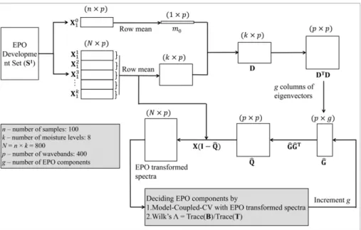
The principle and mathematical implementation of EPO transforma-tion were covered in detail inRoger et al. (2003). For the completeness of the article, a summary is given below. Aﬂow diagram is given inFig. 2, with the important matrices and parameters being annotated.

EPO assumes that spectra matrixXcan be decomposed into two sys-tematic components: a useful componentXPand a parasitic component XQ, as indicated in Eq.(1).Ris the noise component originated from lack ofﬁtting.

X¼XPþXQþR ð1Þ

The procedure toﬁndXPis through spectra matrixD, which is the difference between the spectra matrix with and without external inﬂ u-ence.Qis estimated through singular value decomposition ofD, andXP is then calculated asX(I−Q);Iis the identity matrix.

One of the most important parameters to be determined during EPO development is the number of EPO componentsg(the same notation as inRoger et al. (2003)andMinasny et al. (2011);Ge et al. (2014)usedc for the same meaning).Roger et al. (2003)suggested two methods to determineg: (1) Cross validation of PLS calibration on transformed spectraS1⁎_{(PLS-CV); and (2) calculating Wilk's}_Λ_{of the transformed} spectraS1⁎_as:

Wilk0s Λ¼Trace_Traceð Þ_{ð Þ}B_T ð2Þ

whereTis the variance–covariance matrix of the EPO transformed spectraS1⁎_{, and}_B_{is the variance}_–_{covariance matrix of}_S1⁎_aggregated by sample (i.e., averaging across all moisture levels for each sample).

In PLS-CV, there is optimal coupling betweengand PLS latent vari-able nLV(Roger et al., 2003; Minasny et al., 2011; Ge et al., 2014). This optimal coupling is found by a certain combination ofgand nLVthat gives minimum RMSE in cross validation. We hypothesized that this op-timal coupling might be more important for the nonlinear modeling techniques of RF, ANN, and SVM. Therefore we extend PLS-CV to these three nonlinear modeling techniques by coupling one important tuning parameter for each modeling technique with EPO through cross valida-tion. Instead of PLS-CV, we refer to it as Model-Coupled-CV. The para-graph below gives the detail on the procedure.

All the nonlinear modeling techniques have tuning parameters anal-ogous to nLVin PLS. The major tuning parameters are mtry(the number of variables randomly sampled as candidates at each tree node split) for RF,s(the number of nodes in the hidden layer) for ANN, andC(the

(4)

number of violations to the margin) for SVM (Hastie et al., 2009; James et al., 2013). In RF, mtrywas varied from 5 to 125 (increment by 15 at each step) toﬁnd the best coupling with EPO. In ANN,swas allowed to vary 1 to 9 (step 2) for EPO coupling. In SVM,Cwas varied from 8 to 64 (increment by 8 at each step). In all three nonlinear modeling techniques,gwas allowed to vary from 1 to 10, and the optimal coupling was found by searching for the best combination ofgand the respective coupling parameters (mtry,s, andC) that gives the lowest RMSECV(Root Mean Squared Error of cross validation).

3. Results and discussion

The effect of moisture on soil VNIR reflectance spectra has been doc-umented in several previous publications such asLobell and Asner (2002);Zhu et al. (2010), andMinasny et al. (2011). Ourfindings are consistent to these studies. In general, there is a systematic decrease in soil reflectance with increasing moisture content. The shift is, howev-er, not uniform along the wavelengths. The decrease between two neighboring moisture levels is more pronounced and well separated at the longer wavelengths than shorter wavelengths. This can be attrib-uted to the general lower re_flectance of dry ground soil in the visible re-gion than the NIR rere-gion. Based on this phenomenon,Lobell and Asner (2002)suggested that longer wavelengths are more suited to observe moisture effect on spectra and estimate moisture content.

3.1. Model-coupled-CV versus Wilk'sΛto determine the optimal number of EPO components g

The characteristic of the EPO transformation matrixPis dependent on the number of EPO componentsg. In this study EPO components were determined by two methods: Model-Coupled-CV and Wilk's_Λ. A key difference between the two methods is that Model-Coupled-CV considers the cross validation of model calibration on the transformed spectraS1⁎(Fig. 2). This meansgis dependent on two factors: (1) the coupling between model calibration and EPO, and (2) the response var-iable Y. Conversely, Wilk'sΛonly results in one value ofgregardless of these two factors. AsRoger et al. (2003)pointed out, Wilk'sΛis a cluster separation measurement where it measures the potential classiﬁcation in a group of samples. Before EPO transformation, models are usually poor because the spectra of the same sample at different moisture levels (intra-sample variation) could differ more than the spectra of two dif-ferent samples (inter-sample variation). If the transformation is

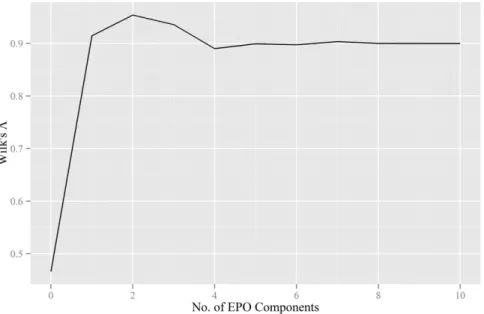
successful in removing or minimizing the moisture effect, different sam-ples should be well separated from the viewpoint of classiﬁcation in the spectral space (Roger et al., 2003). Larger Wilk'sΛimplies better separa-tion of samples.Fig. 3shows Wilk's_Λas a function of the number of EPO components, which suggests thatgis 2 for our dataset.

Table 2givesgdetermined by Model-Coupled-CV and Wilk'sΛ methods for the four modeling techniques with their respective cou-pling parameter. For PLS (the only linear modeling technique),granges from 8 to 10, larger than 2 as determined by Wilk'sΛ. At the same time, the coupling parameter nLVis also smaller for all soil properties (except for Sand). This indicates that, for PLS, Wilk'sΛleads to more parsimoni-ous models for EPO correction and prediction.

An examination of other three nonlinear modeling techniques in

Table 2reveals more interesting pattern. The CV method coupled with RF and SVM yieldedgvalues of either 1 or 2 for all eight soil properties. This is in agreement withFig. 3where Wilk'sΛincreases from 0.47 (g= 0) to 0.92 (g= 1), peaks at 0.95 (g= 2), then decreases and_ﬂuctuates around 0.90 (g= 3 to 10). This indicates wheng= 1 or 2, the separation of spectra between different moisture levels are best; and modeling of EPO transformed spectra with RF and SVM favors lowergwith cross val-idation. ANN modeling gives highergthan RF and SVM with cross vali-dation (but still lower than PLS for OC, IC, and TC).

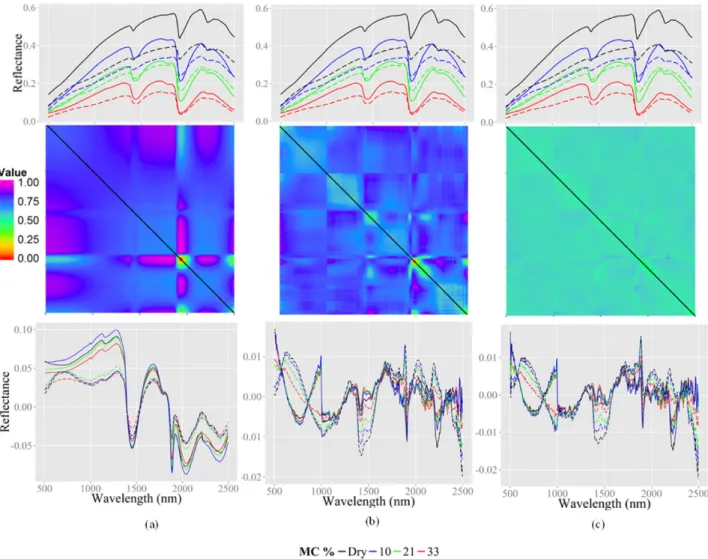
Fig. 4visualizes EPO transformation for different g, by Model-Coupled-CV and Wilk'sΛmethods. The top and bottom rows are the original and EPO-transformed spectra at selected four levels of mois-ture. The mid row shows thePmatrices that resulted from differentg. As previously shown,gdetermined by Wilk'sΛis 2, and those deter-mined by Model-Coupled-CV range from 1 to 10. Here only the transfor-mations withgequal to 2, 6 and 9 are shown.

Fig. 4shows that EPO effectively removes the variability in soil re-ﬂectance spectra caused by moisture, yielding much similar spectra of the same sample after EPO transformation. One striking pattern re-vealed inFig. 4is that the transformation withg= 2 (Fig. 4a) gave a much smoother transformed spectra, comparing to the noisy spectra by higher EPO components (Fig. 4b and c). The primary reason, as we speculate, is that higher EPO components by including a large number of eigenvectors from the decomposition of theDT_D_{matrix could} poten-tially introduce extra spectral noise into parasitic matrixQ(a similar ef-fect as in principal component analysis where higher principal components are usually associated with noise). This in turn makes the EPO projection matrixPnoisier (P=I−Q). In addition, it is quite clear inFig. 4that the two soil samples are better separated when

Fig. 2.Implementation of external parameter orthogonalization (EPO) transformation with the model-coupled-Cross Validation (model-coupled-CV) and Wilk'sΛmethod. The matrix symbols drawn in theﬁgure are for the understanding of matrix operations in the EPO procedure.

(5)

g= 2 compared tog= 6 and 9. We reason that the smoother spectra, together with the better between-sample spectral separation (both achieved wheng= 2), lend the transformed spectra amenable to devel-op moisture insensitive soil prdevel-operty models.

3.2. Comparison of EPO modeling for different soils properties and modeling techniques

Table 3gives the validation result of dry ground models (Model A fromS0_{) for predicting zero moisture spectra of test set (}_S2_{) for the} eight soil properties with the four modeling techniques. It shows that, for our dataset, OC, IC, and TC can be predicted reasonably accurately with R2_{ranging from 0.56 to 0.88 and RPIQ from 1.79 to 2.64. The dry} ground models for clay and sand vary signiﬁcantly among the modeling techniques. They are best predicted with PLS; but their modeling with

RF, ANN and SVM is somewhat poor. The models for pH, P, and CEC are quite poor, with R2_{lower than 0.35. This is consistent with the} liter-ature: VNIR models for soil carbon contents and textures are usually su-perior to other properties such as pH, P and CEC (Stenberg et al., 2010).

Table 4gives the results of model performance with EPO (prediction B inFig. 1) and without EPO (prediction A inFig. 1) for the eight soil properties and four modeling techniques studied. Again, EPO transfor-mation was implemented with two methods: Model-Coupled-CV and Wilk'sΛ. Note that R2_{, RPIQ and RMSE}

PinTable 4were calculated using all eight moisture levels inS2_{. For prediction A, it can be seen} that all predictions fail as indicated by low R2, RPIQ and high RMSE. For OC, IC, and TC, EPO effectively removes the moisture effect and yielded signiﬁcant improvement in prediction for all four modeling techniques. Note that TC, OC, and IC also have the highest accuracy for the initial dry ground models inTable 3. Consistent improvement by EPO is observed for sand with the decreasing of RMSEPvalues, although the improvement is quite marginal. Clay shows improvement only with PLS, but not with other three techniques. For pH, P, and CEC, no im-provement was achieved. When comparing these ﬁndings with

Table 3, it appears that a good initial dry ground model is quite impor-tant for EPO to work. This is not surprising. EPO in principle is an infor-mation removal process that removes spectral components associated with moisture. If the initial dry ground model is poor, meaning a weak correlation between certain soil property and spectra, EPO would not make the correlation stronger (because no spectral information is added).

Since EPO works best for OC, IC and TC, our discussions in the follow-ing focus on these three properties. A cross comparison between

Tables 2and4provides us some insight on how differently EPO couples the linear (PLS) and nonlinear (RF, ANN, and SVM) techniques. For PLS, gas determined by PLS-CV is much larger than Wilk'sΛ. But the predic-tion result inTable 4shows that the performance is superior with Wilk's Λfor OC and IC, and only slightly inferior for TC. Largergseems not ben-eﬁcial to improvement the EPO modeling performance. This is in agree-ment withFig. 4where EPO-transformed spectra from lowergare much smoother. For ANN, the same pattern can be seen between ANN-CV and Wilk'sΛ(smallergandsbut comparable model performance). For RF and SVM, it is notable that their CV gives the almost sameg(1 or 2) as Wilk'sΛ. From these analyses it seems that the nonlinear modeling techniques can be better coupled with EPO through cross validation, as they yieldedgcomparable to Wilk'sΛ(which we know is better as seen inFig. 3) and better model performance than PLS.

Fig. 3.Wilk'sΛas a function of the number of external parameter orthogonalization (EPO) componentsg(zero component means no EPO transformation). Higher Wilk'sΛindicates a higher degree of separation of different samples with respect to the same sample of different moisture levels in the spectral space.

Table 2

Optimum number of external parameter orthogonalization (EPO) components (g) and the coupling parameters for the four modeling techniques determined by the Model-Coupled-CV and Wilk'sΛmethod.

Modeling Technique EPO method Tuning parameter Soil property

OC IC TC Sand Clay pH P CEC

PLS PLS-CV nLV 15 20 10 20 20 20 20 20 g 9 10 9 9 9 8 8 10 Wilk'sΛ nLV 11 14 5 22 12 20 5 15 g 2 2 2 2 2 2 2 2 RF RF-CV mtry 110 5 125 35 125 20 125 125 g 1 1 1 2 2 1 1 2 Wilk'sΛ mtry 50 125 110 20 125 80 5 65 g 2 2 2 2 2 2 2 2 ANN ANN-CV s 5 9 5 5 3 5 5 9 g 6 7 4 10 10 6 9 9 Wilk'sΛ s 1 1 3 3 1 1 1 7 g 2 2 2 2 2 2 2 2 SVM SVM-CV C 64 64 64 64 64 64 64 64 g 1 1 1 1 1 1 1 1 Wilk'sΛ C 64 64 64 64 64 64 64 64 g 2 2 2 2 2 2 2 2

PLS is Partial Least Squares Regression; RF is Random Forest; ANN is Artiﬁcial Neural Net-works; SVM is Support Vector Machine.

P is Mehlich-3 Phosphorus; CEC is Cation Exchange Capacity.

nLVis the number of PLS latent variables;gis number of EPO components; mtryis the num-ber of variables randomly sampled as candidates at each split in RF modeling;sis the num-ber of nodes in the hidden layer in ANN modeling; and C is the severity of the violations to the margin in SVM modeling.

(6)

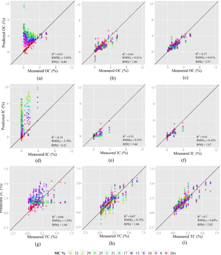
Fig. 5provides a pictorial view of how EPO improves modeling for samples at different moisture levels.Fig. 5a to c show OC prediction with ANN. It can be seen that, without EPO (Model A applied directly

toS2_{), as moisture level increases, the prediction becomes poorer as} suggested by increasing deviation from 1:1 line. The lack of linear re-sponse and a systematic over prediction indicate that the variation in spectra is dominated by moisture, thus failing OC prediction, particular-ly at higher moisture levels.Fig. 5b and c are predictions with ANN-CV and Wilk'sΛ, respectively. It is obvious that the prediction with EPO greatly improve the linear response of predictions across all moisture levels, resulting in signiﬁcant improvement in model statistics (R2, RPIQ, and RMSEP). Same patterns are observed for IC prediction with PLS (Fig. 5d–f); and TC with SVM (Fig. 5g–i) modeling. The variation in-duced by moisture was greatly suppressed, resulting in strong linear re-sponses to the respective soil properties and minimal differences across different moisture levels.

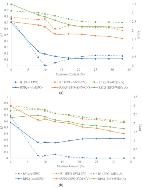
3.3. The performance of EPO across different moisture levels

Infield applications, soils will be at differentfield moisture levels. Therefore it is an important question to ask if EPO performs equally well across different moisture levels.Fig. 6gives the summary statistics of R2_{(on the left Y axis) and RPIQ (on the right Y axis) as a function of} moisture level for OC prediction with ANN (Fig. 6a) and TC prediction with SVM (Fig. 6b). Without EPO, both R2_{and RPIQ drop very quickly} from 0 (dry ground) to 8% moisture (thefirst level) and remain low for higher moisture levels. With the EPO transformation, models still predict best for 0 moisture, but only drop slowly from 0 to the next three moisture levels (8, 10, 13%) and then level off at higher moisture

Fig. 4.Visualization of external parameter orthogonalization (EPO) transformation with two (a), six (b) and nine (c) EPO components. Solid and dash lines represents two different soil samples while black, red, green and blue colors represent different soil moisture levels.

Table 3

The validation results of dry ground models (Model A fromS0

inFig. 1) to predict for the dry ground spectra of test set (zero moisture inS2

) for the eight soil properties with four modeling techniques.

Modeling technique

Parameter Soil property

PLS R2 _0.71 _0.81 _0.67 _0.55 _0.44 _0.08 _0.12 _0.24 RPIQ 2.03 2.59 1.79 1.41 0.89 1.24 1.10 1.04 RMSEP 0.74 0.31 0.78 20.22 12.54 1.29 38.97 6.61 RF R2 0.76 0.73 0.64 0.00 0.16 0.35 0.11 0.12 RPIQ 2.05 2.09 1.82 0.99 1.32 1.93 1.11 1.06 RMSEP 0.73 0.38 0.77 29.00 8.51 0.83 38.78 6.54 ANN R2 0.76 0.79 0.88 0.40 0.27 0.07 0.05 0.23 RPIQ 2.46 2.58 2.64 1.58 0.91 0.67 0.99 1.01 RMSEP 0.61 0.31 0.53 18.09 12.25 2.39 43.22 6.85 SVM R2 0.77 0.56 0.69 0.26 0.15 0.07 0.03 0.08 RPIQ 2.50 1.81 2.03 1.36 1.11 1.38 1.02 0.99 RMSEP 0.60 0.44 0.69 21.03 10.07 1.16 41.94 6.97 PLS is Partial Least Squares Regression; RF is Random Forest; ANN is Artiﬁcial Neural Net-work; and SVM is Support Vector Machine.

P is Mehlich-3 Phosphorus; CEC is Cation Exchange Capacity.

(7)

levels. This shows that EPO can substantially improve prediction for all moisture level. Inﬁeld applications, it is expected that EPO has the po-tential to be used for a wide range ofﬁeld moist samples, and there would be a slight decrease in prediction performance for higher mois-ture soils than lower moismois-ture soils.

4. Conclusions

We conducted an in-depth study of EPO for removing moisture ef-fect from soil VNIR spectra and improving model performance. We ex-panded the investigation to eight soil properties and four different modeling techniques. We also compared the two methods for deter-mining the optimum number of EPO componentsg: model-coupled-CV and Wilk'sΛ. The major conclusions drawn from this study are as follows.

1. EPO is effective in removing moisture effect from soil VNIR spectra at different moisture levels. Its effectiveness can be readily seen by comparing the spectra before and after EPO transformation. Before transformation, the variation induced by moisture is so large that it masks the variation between samples. After EPO transformation, moisture-induced variation was largely suppressed and between-sample variation becomes dominant again.

2. Wilk'sΛis a viable method for determiningg. Compared to model-coupled-CV, Wilk'sΛonly relies on reﬂectance spectra forg determi-nation and yields smoother spectra after transformation. With PLS, Wilk'sΛgenerally gives rise to lowergand nLVthan PLS-CV for all soil properties, indicating its advantage in model parsimony. For the nonlinear modeling techniques, their respective CV methods tend to favor smallergcomparable to the Wilk'sΛmethod (especial-ly for RF and SVM). The coupling between EPO and these nonlinear modeling techniques is superior to PLS.

3. Among the eight soil properties, EPO improved the prediction of OC, IC, and TC signiﬁcantly. The prediction of sand and clay, were im-proved only marginally, and the improvement is not consistent among different modeling techniques. For the predictions of pH, Mehlich-3 P, and CEC, EPO did not show improvement. Having good initial dry ground models is important for EPO to work. 4. For OC, IC, and TC, EPO substantially improves prediction at all

differ-ent moisture levels. However, there is a slight decrease in the predic-tion accuracy when samples have higher moisture contents.

Acknowledgments

This work was funded by the U.S. Department of Agriculture— Natural Resources Conservation Services. The authors would like

Table 4

Results of model performance using moist soil VNIR spectra without (A) and with (B) external parameter orthogonalization (EPO) for predicting the eight soil properties ofS2_{set by using} four modeling techniques.

Modeling technique Prediction Parameter Soil property

PLS A R2 _0.11 _0.19 _0.03 _0.13 _0.00 _0.04 _0.00 _0.04 RPIQ 0.31 0.21 0.20 0.32 0.12 0.30 0.57 0.38 RMSEP 4.80 3.78 6.87 88.83 94.78 5.36 74.63 17.97 B/PLS-CV R2 0.08 0.31 0.51 0.27 0.01 0.04 0.08 0.08 RPIQ 1.10 1.44 1.49 1.33 0.72 1.49 1.02 0.67 RMSEP 1.36 0.55 0.94 21.58 15.60 1.08 42.00 10.34 B/Wilk'sΛ R2 _0.56 _0.61 _0.29 _0.20 _0.00 _0.00 _0.11 _0.08 RPIQ 1.77 1.87 1.31 1.25 0.48 0.87 1.09 0.64 RMSEP 0.85 0.43 1.07 22.83 23.19 1.84 39.39 10.80 RF A R2 0.19 0.05 0.07 0.00 0.09 0.12 0.04 0.01 RPIQ 0.56 0.99 0.62 0.73 1.01 1.53 1.21 0.59 RMSEP 2.70 0.81 2.26 39.23 11.09 1.05 35.49 11.71 B/RF-CV R2 0.63 0.70 0.55 0.19 0.01 0.21 0.02 0.08 RPIQ 1.89 1.96 1.64 1.51 0.78 1.73 0.90 0.75 RMSEP 0.79 0.41 0.85 18.98 14.45 0.92 47.89 9.19 B/Wilk'sΛ R2 0.61 0.71 0.55 0.18 0.01 0.12 0.02 0.08 RPIQ 1.86 1.82 1.65 1.52 0.77 1.65 0.94 0.76 RMSEP 0.81 0.44 0.85 18.76 14.46 0.97 45.72 9.10 ANN A R2 0.01 0.40 0.24 0.08 0.01 0.00 0.01 0.00 RPIQ 0.49 1.51 0.44 0.54 0.64 0.65 0.83 0.44 RMSEP 3.05 0.53 3.19 52.95 17.39 2.48 51.57 15.74 B/ANN-CV R2 0.64 0.68 0.71 0.11 0.02 0.12 0.02 0.09 RPIQ 1.86 2.08 2.11 1.21 0.78 1.52 0.75 0.69 RMSEP 0.81 0.38 0.66 23.58 14.45 1.05 56.95 10.00 B/Wilk'sΛ R2 0.77 0.32 0.64 0.16 0.00 0.00 0.01 0.06 RPIQ 2.47 1.45 1.86 1.22 0.69 0.88 1.12 0.72 RMSEP 0.61 0.55 0.75 23.50 16.22 1.81 38.22 9.63 SVM A R2 _0.12 _0.08 _0.06 _0.04 _0.03 _0.06 _0.02 _0.00 RPIQ 1.19 1.05 1.04 0.60 1.06 1.31 1.15 0.91 RMSEP 1.27 0.76 1.34 47.55 10.58 1.22 37.30 7.62 B/SVM-CV R2 0.71 0.55 0.67 0.11 0.00 0.12 0.00 0.08 RPIQ 1.99 1.61 1.86 1.26 0.52 1.53 0.95 0.56 RMSEP 0.75 0.50 0.75 22.70 21.42 1.05 45.34 12.43 B/Wilk'sΛ R2 _0.75 _0.70 _0.70 _0.18 _0.00 _0.03 _0.01 _0.07 RPIQ 2.40 1.72 2.02 1.37 0.68 1.47 0.94 0.68 RMSEP 0.63 0.46 0.69 20.89 16.54 1.09 45.42 10.17

PLS is Partial Least Squares Regression; RF is Random Forest; ANN is Artiﬁcial Neural Network; SVM is Support Vector Machine. P is Mehlich-3 Phosphorus; CEC is Cation Exchange Capacity.

Prediction method: A means the models are based on the dry ground spectra without EPO correction; B/Model-CV means the EPO models developed from the model-coupled-CV method; B/Wilk'sΛmeans the EPO models developed from the Wilk'sΛmethod.

(8)

to thank the staff at Kellogg Soil Survey Lab (Dr. Richard R. Ferguson, Scarlett Bailey and Michael J. Pearson) for their assistance in sample retrieval from the archive and VNIR scanning.

References

Ackerson, J.P., Demattê, J.A.M., Morgan, C.L.S., 2015.Predicting clay content onﬁeld-moist intact tropical soils using a dried, ground VisNIR library with external parameter or-thogonalization. Geoderma 259–260, 196–204.

Fig. 5.Prediction of different soil properties with and without external parameter orthogonalization (EPO) transformation. First, second and third rows correspond to Organic C with ANN, Inorganic C with PLS, and Total C with SVM modeling respectively. First, second and third columns correspond to prediction plots without EPO transformation, EPO transformation with Model-coupled-CV method, and EPO transformation with Wilk'sΛmethod.

(9)

Bellon-Maurel, V., Fernandez-Ahumada, E., Palagos, B., Roger, J.-M., McBratney, A., 2010. Critical review of chemometric indicators commonly used for assessing the quality of the prediction of soil attributes by NIR spectroscopy. TrAC Trends in Analytical Chemistry 29 (9), 1073–1081.

Ben-Dor, E., Heller, D., Chudnovsky, A., 2008.A novel method of classifying soil proﬁles in theﬁeld using optical means. Soil Sci. Soc. Am. J. 72 (4), 1113–1123.

Bricklemyer, R.S., Brown, D.J., 2010.On-the-go VisNIR: potential and limitations for mapping soil clay and organic carbon. Comput. Electron. Agric. 70 (1), 209–216.

Brown, D.J., Shepherd, K.D., Walsh, M.G., Dewayne Mays, M., Reinsch, T.G., 2006.Global soil characterization with VNIR diffuse reﬂectance spectroscopy. Geoderma 132 (3–4), 273–290.

Chang, C.-W., Laird, D.A., Mausbach, M.J., Hurburgh, C.R., 2001.Near-infrared reﬂectance spectroscopy–principal components regression analyses of soil properties. Soil Sci. Soc. Am. J. 65 (2), 480–490.

Core Team, R., 2015.R: A Language and Environment for Statistical Computing. R Founda-tion for Statistical Computing, Vienna, Austria.

Ge, Y., Thomasson, J.A., Morgan, C.L., Searcy, S.W., 2007.VNIR diffuse reﬂectance spectros-copy for agricultural soil property determination based on regression-kriging. Trans. ASABE 50 (3), 1081–1092.

Ge, Y., Morgan, C.L.S., Ackerson, J.P., 2014.VisNIR spectra of dried ground soils predict properties of soils scanned moist and intact. Geoderma 213, 61–69.

Gomez, C., Viscarra Rossel, R.A., McBratney, A.B., 2008.Soil organic carbon prediction by hyperspectral remote sensing andﬁeld vis-NIR spectroscopy: an Australian case study. Geoderma 146 (3–4), 403–411.

Hastie, T., Tibshirani, R., Friedman, J., 2009.The Elements of Statistical Learning, 2. Springer.

James, G., Witten, D., Hastie, T., Tibshirani, R., 2013.An Introduction to Statistical Learning. Springer.

Ji, W., Viscarra Rossel, R.A., Shi, Z., 2015.Accounting for the effects of water and the envi-ronment on proximally sensed vis–NIR soil spectra and their calibrations. Eur. J. Soil Sci. 66 (3), 555–565.

Karatzoglou, A., Smola, A., Hornik, K., Zeileis, A., 2004.Kernlab—an S4 package for kernel methods in R. J. Stat. Softw. 11 (9), 1–20.

Kuang, B., Mouazen, A.M., 2013.Non-biased prediction of soil organic carbon and total ni-trogen with vis–NIR spectroscopy, as affected by soil moisture content and texture. Biosyst. Eng. 114 (3), 249–258.

Max, K., Jed, W., Weston, S., Williams, A., Keefer, C., Engelhardt, A., Cooper, T., Mayer, Z., Kenkel, B., the R Core Team, Benesty, M., Lescarbeau, R., Ziem, A., Scrucca, L., 2015. Caret: classiﬁcation and regression training.

Liaw, A., Wiener, M., 2002.Classiﬁcation and regression by randomForest. R News 2 (3), 18–22.

Lobell, D.B., Asner, G.P., 2002.Moisture effects on soil reﬂectance. Soil Sci. Soc. Am. J. 66 (3), 722–727.

Mevik, B.-H., Wehrens, R., Liland, K.H., 2013.pls: partial least squares and principal com-ponent regression.

Minasny, B., McBratney, A.B., Pichon, L., Sun, W., Short, M.G., 2009.Evaluating near infrared spectroscopy forﬁeld prediction of soil properties. Soil Res. 47 (7), 664–673.

Minasny, B., McBratney, A.B., Bellon-Maurel, V., Roger, J.-M., Gobrecht, A., Ferrand, L., Joalland, S., 2011.Removing the effect of soil moisture from NIR diffuse reﬂectance spectra for the prediction of soil organic carbon. Geoderma 167–168, 118–124. Morgan, C.L.S., Waiser, T.H., Brown, D.J., Hallmark, C.T., 2009.Simulated in situ

character-ization of soil organic and inorganic carbon with visible near-infrared diffuse reﬂ ec-tance spectroscopy. Geoderma 151 (3–4), 249–256.

Mouazen, A.M., De Baerdemaeker, J., Ramon, H., 2005.Towards development of on-line soil moisture content sensor using aﬁbre-type NIR spectrophotometer. Soil Tillage Res. 80 (1), 171–183.

Fig. 6.The performance of external parameter orthogonalization (EPO) correction on (a) soil Organic C with ANN modeling, and (b) Total C with SVM modeling, at different soil moisture levels.

(10)

Nocita, M., Stevens, A., Noon, C., van Wesemael, B., 2013.Prediction of soil organic carbon for different levels of soil moisture using vis-NIR spectroscopy. Geoderma 199, 37–42. Revelle, W., 2015.Psych: procedures for psychological, psychometric, and personality

re-search. Northwestern University, Evanston, Illinois.

Roger, J.-M., Chauchard, F., Bellon-Maurel, V., 2003.EPO–PLS external parameter orthogonalisation of PLS application to temperature-independent measurement of sugar content of intact fruits. Chemom. Intell. Lab. Syst. 66 (2), 191–204. Sarkhot, D.V., Grunwald, S., Ge, Y., Morgan, C.L.S., 2011.Comparison and detection of total

and available soil carbon fractions using visible/near infrared diffuse reﬂectance spec-troscopy. Geoderma 164 (1–2), 22–32.

Shepherd, K.D., Walsh, M.G., 2002.Development of reﬂectance spectral libraries for char-acterization of soil properties. Soil Sci. Soc. Am. J. 66 (3), 988–998.

Sørensen, L., Dalsgaard, S., 2005.Determination of clay and other soil properties by near infrared spectroscopy. Soil Sci. Soc. Am. J. 69 (1), 159–167.

Stenberg, B., 2010.Effects of soil sample pretreatments and standardised rewetting as interacted with sand classes on vis-NIR predictions of clay and soil organic carbon. Geoderma 158 (1–2), 15–22.

Stenberg, B., Viscarra Rossel, R.A., Mouazen, A.M., Wetterlind, J., 2010.Visible and near in-frared spectroscopy in soil science. Adv. Agron. 107, 163–215.

Sudduth, K., Hummel, J., 1993.Soil organic matter, CEC, and moisture sensing with a por-table NIR spectrophotometer. Trans. ASAE (USA).

Venables, W.N., Ripley, B.D., 2002.Modern Applied Statistics with S. fourth ed. Springer, New York.

Viscarra Rossel, R.A., Walvoort, D.J.J., McBratney, A.B., Janik, L.J., Skjemstad, J.O., 2006. Vis-ible, near infrared, mid infrared or combined diffuse reﬂectance spectroscopy for si-multaneous assessment of various soil properties. Geoderma 131 (1–2), 59–75. Waiser, T.H., Morgan, C.L.S., Brown, D.J., Hallmark, C.T., 2007.In situ characterization of

soil clay content with visible near-infrared diffuse reﬂectance spectroscopy. Soil Sci. Soc. Am. J. 71 (2), 389.

Wickham, H., 2009.ggplot2: elegant graphics for data analysis.

Zhu, Y., Weindorf, D.C., Chakraborty, S., Haggard, B., Johnson, S., Bakr, N., 2010. Character-izing surface soil water withﬁeld portable diffuse reﬂectance spectroscopy. J. Hydrol. 391 (1–2), 133–140.