Hyper-and-elliptic-curve cryptography
Daniel J. Bernstein and Tanja Lange
Abstract
This paper introduces “hyper-and-elliptic-curve cryptography”, in which a single high-security group supports fast genus-2-hyperelliptic-curve formulas for variable-base-point single-scalar multiplication (e.g., Diffie–Hellman shared-secret computation) and at the same time supports fast elliptic-curve formulas for fixed-base-point scalar multiplication (e.g., key generation) and multi-scalar multiplication (e.g., signature verification).
Keywords: performance, Diffie–Hellman, elliptic curves, hyperelliptic curves, Weil restriction, isogenies, Scholten curves, Kummer surfaces, Edwards curves
1. Introduction
We would very much like to see forward secrecy become the norm and hope that our deployment serves as a demonstration of the practicality of that vision.
—“Protecting data for the long term with forward secrecy”, 22 November 2011 [38] Forward secrecy is just the latest way in which Twitter is trying to defend and protect the user’s voice. —“Forward secrecy at Twitter”, 22 November 2013 [31]
The classic Diffie–Hellman protocol [17, Section 3] sets up secure communication channels between any number of users as follows. Alice has a long-term secret key aand a long-term public key ga, where g is a standard element of the multiplicative group of a finite field.
Similarly, Bob has a long-term secret keyb and a long-term public keygb; Charlie has a
long-term secret keyc and a long-term public key gc; etc. Alice and Bob each compute gab, which
they use as a long-term key for secret-key cryptography to efficiently encrypt and authenticate messages. Alice and Charlie encrypt usinggac; Bob and Charlie encrypt usinggbc; etc.
This protocol never erases keys, so it does not provideforward secrecy. An attacker who steals Bob’s computer, after recording all network communication, sees gab and gbc and decrypts Bob’s past messages, even if Bob has erased all of the messages. Bob cannot stop this attack by erasinggaband gbc: the attacker simply recomputesgab andgbc fromb. Bob cannot erase
b: Bob needsb to compute shared secrets with new users.
The obvious way to provide forward secrecy is to further encrypt messages using anephemeral
variant of the Diffie–Hellman protocol. Alice and Bob start by setting up a secure channel as above, using Alice’s long-term public key ga and Bob’s long-term public key gb. Then, for
each message from Alice to Bob, Alice generates a one-time secret key r and sends gr to
Bob through the secure channel; Bob also generates a one-time secret key sand sends gs to
Alice through the secure channel. Alice encrypts the message usinggrs, sends the ciphertext
C through the secure channel, and throws away r and grs. Bob decrypts the message using
grs and throws awaysandgrs. An attacker who steals Bob’s computer still has the power to
decrypt the original channel, obtaininggr,gs, andC, but there is no obvious way to recover
2000Mathematics Subject Classification11G20, 14G50, 94A60.
the original message. Of course, the attack compromises the confidentiality and integrity of
future messages, butpast messages are still protected.
Notice that the ephemeral Diffie–Hellman protocol has different performance characteristics from the original protocol. In the original protocol, the dominant computation is a variable-base exponentiationa, gb7→gab: for U users Alice does U variable-base exponentiations gab, gac, etc. and only one fixed-base exponentiationa7→ga. InM runs of the ephemeral protocol, Alice performs M fixed-base exponentiations r7→gr and M variable-base exponentiations
r, gs7→grs, so Alice benefits significantly from speedups in either type of exponentiation. One
can consider intermediate possibilities, such as reusing an ephemeral key for several messages, but forward secrecy is strongest when a key is discarded immediately after its first use.
1.1. Elliptic curves and hyperelliptic curves
Modern cryptography replaces the multiplicative groups in DH with elliptic-curve groups, as proposed by Miller [40] and independently by Koblitz [36]. This loses an important constant factor in the number of field operations required for a group operation, but it gains much more from avoiding index-calculus attacks. Specifically, to achieve a security level around 2128, elliptic-curve groups use base fields of size around 2256, while multiplicative groups need base fields of size around 23000. See, e.g., [28].
The recent paper [6] by Bos, Costello, Hisil, and Lauter shows that for high-security DH one obtains even better performance from a different option: Jacobian groups of hyperelliptic curves of genus 2. The main advantage of genus 2 over genus 1 is that a much smaller base field, specifically a field of size around 2128, produces a group of size around 2256and a security level around 2128. Reducing the number of bits in the field by a factor of 2 typically produces a speedup factor around 3, depending on various details of field arithmetic. The disadvantage of genus 2 is that each group operation requires many more field operations; but for Gaudry’s [24] Kummer-surface formulas this loss factor is only slightly above 2. Even better, 24% of Gaudry’s field multiplications are multiplications by curve parameters that can be chosen to be small; a secure small-parameter genus-2 curve was announced by Gaudry and Schost [27] after a massive point-counting computation. A further advantage of genus 2, exploited in a very recent paper [4] by Bernstein, Chuengsatiansup, Lange, and Schwabe, is a synergy between the structure of Gaudry’s formulas and the availability of vector operations in modern CPUs. One can speed up genus 1 using “time” addition chains. However, non-constant-time computations are a security problem; see, e.g., the attacks cited in [4, Section 1.2].
One can also speed up genus 1 by applying endomorphisms on suitably chosen curves: e.g., rewritingaP asa0P+a1φ(P) wherea0anda1have half as many bits asa. See, e.g., [19] and [44]. Analogous ideas in genus 2 seem less effective; see [7]. However, endomorphisms in this context are patented, and are thus not helpful for users concerned with the real-world cost of cryptography. Furthermore, even with this speedup, genus 1 is not as fast as genus 2; see [4].
1.2. Hyperelliptic curves and forward secrecy
The comparison between genus 1 and genus 2 changes when one switches from classic DH to ephemeral DH. Genus 2 is the speed leader for variable-base scalar multiplicationr, sG7→rsG, but genus 1 is the speed leader for fixed-base scalar multiplicationr7→rG, and for forward secrecy both operations are important. There is some speedup from variable base to fixed base in genus 2 (see [6] for a detailed analysis), but there is a much larger speedup in genus 1. We summarize the relative time required for each operation as follows:
fixed-base genus 1<fixed-base genus 2<variable-base genus 2<variable-base genus 1.
means slowing down key generation. Choosing genus 1 means slowing down the computation of a shared secret.
To resolve this problem we propose using public keys in a group that can be viewed simultaneously as a genus-1 group and a genus-2 group. More precisely, assume that we have
• an elliptic curve E over Fp2, specifically (for speed and simplicity) an Fp2-complete
Edwards curve;
• the JacobianJ of a genus-2 hyperelliptic curve overFp, specifically one supporting a fast
(i.e., small-parameter) Kummer surface; and
• an efficientFp-isogeny fromW toJ, whereW is the Weil restriction ofE fromFp2 toFp.
Setting up this situation is the main work in this paper. Alice then uses fast elliptic-curve formulas for fixed-base scalar multiplication to generate a public keyrGinE(Fp2) =W(Fp).
Either Alice or Bob applies the isogeny to rG, obtaining an equivalent public key in J(Fp).
Bob then uses fast Kummer-surface formulas to compute a shared secret inJ(Fp). We suggest
having Bob apply the isogeny, since uncompressing a compressed elliptic-curve point is simpler than uncompressing a compressed Kummer-surface point.
Of course, one can also use the dual isogeny to map fromJ(Fp) back toE(Fp2). However, it
seems natural to start withE(Fp2), since elliptic-curve formulas are very fast for key generation.
The obvious general strategy is to use Edwards coordinates onE(Fp2) for computations where
those formulas are fastest, and to use Kummer coordinates onJ(Fp) for computations where
those formulas are fastest, using the isogenies to convert whenever necessary.
Any further evolution of coordinate systems and formulas can of course be integrated into the same picture. It seems reasonable to speculate that neither genus 1 nor genus 2 will end up as a clear winner, so the ability to mix genus 1 and genus 2 will remain useful.
1.3. Further applications
Our approach is applicable to many contexts in which different types of scalar multiplication are mixed; forward secrecy is obviously an important application but there are other applications. For example, there are safe methods to use a single element of a group of order approximately 2256 as a long-term public key for both DH and signatures; see, e.g., [29], [45], and [13]. Using two separate keys, one for DH and one for signatures, means transmitting both of those keys, and in some settings also transmitting a signature of the DH key under the signing key; a single key is clearly much more satisfactory. With our techniques, this single key allows fast genus-1 formulas for key generation, signing, and signature verification while simultaneously allowing fast genus-2 formulas for DH shared-secret computation. If signing and signature verification are much more frequent than encryption then the genus-1 operations will be dominant, but in general one should expect many different levels of balance between the genus-1 operations and the genus-2 operations.
A further advantage of genus 1 for signature verification is that there are no exceptional cases in the standard addition law for E(Fp2) when E is an Fp2-complete Edwards curve.
For comparison, all fast genus-2 addition laws in the literature have exceptional cases. Using genus-1 addition by default, and moving to a genus-2 ladder for shared-secret computation, means that we avoid all of these exceptional cases.
1.4. Notes regarding terminology
It is slightly sloppy to refer to “the” Weil restriction. There are actually many different choices of Weil restrictions, corresponding to different choices of a basis (b0, b1) forFp2 overFp:
specifically, the affine part ofW is the set of (x0, x1, y0, y1) such that (x0b0+x1b1, y0b0+y1b1) is a point onE. Modifying (b0, b1) produces a linearly isomorphic but not identical variety. If we were defining and evaluating the efficiency ofFp-algebraic algorithms for computing the rational
maps that appear in this paper then we would need this extra level of mathematical precision; fortunately, all of the maps that we present are clearly much faster than scalar multiplication, so a detailed cost evaluation is unnecessary. Related choices do become important in Section 6, where we choose ∆ and lift the whole picture toQ(√∆).
2. Weierstrass to genus-2 Jacobian: efficient isogenies for Scholten curves
We do not claim credit for the fact that one can construct elliptic curves overFp2 isogenous
(after restriction of scalars) to genus-2 Jacobians overFp: we reuse a construction published
by Scholten ten years ago in [48]. Scholten credits to Diem the case that E has full 2-torsion defined overFp2, but Scholten’s construction is simpler than Diem’s construction.
Scholten’s goal was to write down hyperelliptic curves that allowed fast point-counting. By constructing curves so that the Weil restriction W of the elliptic curve from Fp2 to Fp is
isogenous to the JacobianJ of a genus-2 hyperelliptic curve overFp, Scholten guaranteed that
#J(Fp) = #W(Fp) = #E(Fp2). See [48, Lemma 2.1]. Counting points on elliptic curves is
reasonably fast, producing #E(Fp2) and thus the desired #J(Fp).
The idea of fast point-counting on genus-2 curves by constructive Weil restriction was introduced by Gaudry, Hess, and Smart in [26], but the constructions in [26] were limited to characteristic 2; odd characteristic was called “hard” in [26, Section 7.2] and “rather difficult” in [23, Section 7]. Various odd-characteristic constructions appeared in [14], [15], [48], [51], and [16]. Special cases with extra small-norm endomorphisms were used in [47] and [21]. Many of these papers feature “Weil-descent attacks” and “cover attacks” as another application of Weil restriction, as suggested by Frey in [22]; Weil-descent attacks using Scholten curves appeared in [2], [41], and [33].
We do claim credit for the idea of using an isogeny to convert keys betweenEandJ, making cryptography faster. At this point one can and should object that [48, Lemma 2.1] merely guarantees the existence of an isogeny fromW to J; it does not guarantee the existence of an
efficientisogeny fromWtoJ. For most pairs of isogenous Abelian varieties, the fastest isogenies known are much slower than scalar multiplication. (This was not an issue for Scholten: any isogeny, no matter how slow, is adequate to show that #J(Fp) = #W(Fp). It was also not a
serious issue for attack papers such as [2]: the use ofJin [2] was for carrying out a Weil-descent attack against E, and other steps of this attack were much more expensive.) This could be fatal for our idea of applying an isogeny on demand.
The main challenge addressed in this section is to show that W and J are efficiently
isogenous. We exhibit efficient formulas for an isogenyι:W →J and efficient formulas for an isogenyι0 :J →W, and show that the composition ofι0 and ιis the doubling map. Section 3 explains how we computed these formulas. Sections 4, 5, and 6 tackle additional challenges in curve construction, with the goal of accelerating group operations inE(Fp2) and inJ(Fp).
2.1. Review of the Scholten curves
Fix an odd prime p. Scholten’s construction begins with an elliptic curve E over Fp2
of the form y2=rx3+sx2+spx+rp, where r, s∈Fp2. Scholten also takes two additional
rpβ66= 0, and observes that
r(α−αβpz)6+s(α−αβpz)4(1−βz)2+sp(α−αβpz)2(1−βz)4+rp(1−βz)6=ω2f
for some nonzeroω∈Fp2 and some monic degree-6 polynomialf ∈Fp[z]. Scholten proves that
the JacobianJ of the hyperelliptic curvey2=f(z) overF
pis isogenous to the Weil restriction
W ofE.
Note that Scholten has more parameters than necessary: replacing (r, s, α, β) with (rα3, sα,1, β) produces an isomorphic elliptic curve and the same hyperelliptic curve. We therefore simplify the formulas by takingα= 1: from now on
r(1−βpz)6+s(1−βpz)4(1−βz)2+sp(1−βpz)2(1−βz)4+rp(1−βz)6=ω2f
andr(βp)6+s(βp)4β2+sp(βp)2β4+rpβ66= 0.
Scholten showed in [48, Section 3] that all elliptic curves over Fp2 with full 2-torsion are
isogenous to Scholten curves. Any general security problem with the algebraic structure of Scholten curves would therefore imply serious trouble for ECC overFp2.
Note that the characteristic polynomial for J is even, sinceχJ(t) =χE(t2). This
automat-ically implies twist-security for J: the twist of J has the same number of points as J, even thoughJ is usually not supersingular. This does not imply twist-security forE.
2.2. A numerical example
We use the following cryptographically strong example as a running example throughout the paper. Most of our computations used the free Sage [49] computer-algebra system, but we are not aware of any free software for fast point-counting on elliptic curves over quadratic extensions of large prime fields, so for point-counting we used the Magma [8] computer-algebra system.
Define pas the prime 2127−309. Note that p∈3 + 4Z; defineF
p2 asFp[i]/(i2+ 1). Define
r= (7 + 4i)2= 33 + 56i and s= 159 + 56i; note that rp= 33−56i and sp= 159−56i. The
elliptic curvey2=rx3+sx2+spx+rp has 16`points overF
p2, where` is the prime number
1809251394333065553493296640760748553649194606010814289531455285792829679923
slightly below 2250, providing roughly 2125 security against conventional discrete-logarithm attacks. The order of ` in (Z/p)∗ is 12152941675747802266549093122563150387, providing ample security against index calculus. The prime factorization of the number of points on the twist of this curve overFp2 is
22·3·7·48862393571594394667013
·9001629735747854493654841·783508531819706590448910673,
providing roughly 275 security against active twist attacks.
Define β=i and ω= 54570365625747840813365101134244818327. Then β2=−1, (βp)2= −1, and ω2=−384 in F
p, so r(βp)6+s(βp)4β2+sp(βp)2β4+rpβ6=−r−s−sp−rp= −384 =ω2. The Scholten curve with parametersr, s, βisy2=f(z) withf(z) =z6+ (7/3)z5− (7/4)z4−(14/3)z3+ (7/4)z2+ (7/3)z−1.
2.3. Explicitly mappingW toJ
Figures 2.4 and 2.5 exhibit formulas for our efficient rational mapιfrom the Weil restriction of an elliptic curve to the Jacobian of a Scholten curve. See Section 2.6 for a proof that this rational map is an isogeny.
R1 = ZZ
P1.<polyi> = R1[]
R2.<i> = P1.quotient(polyi^2+1)
r,s,b = 33+56*i,159+56*i,i rp,sp,bp = 33-56*i,159-56*i,-i
ww = R1(r*bp^6+s*bp^4*b^2+sp*bp^2*b^4+rp*b^6) R2z.<z> = R2[]
wwf = r*(1-bp*z)^6+s*(1-bp*z)^4*(1-b*z)^2+sp*(1-bp*z)^2*(1-b*z)^4+rp*(1-b*z)^6 f = wwf.change_ring(R1) / ww
P1.<X0,X1,Y0,Y1> = R1[] P2 = P1.change_ring(R2) X = P2(X0)+P2(X1)*i Yw = P2(Y0)+P2(Y1)*i
curve = r*X^3+s*X^2+sp*X+rp-ww*Yw^2
curvereal = curve.map_coefficients(lambda u:u[0]).change_ring(R1) curveimag = curve.map_coefficients(lambda u:u[1]).change_ring(R1) assumptions = (curvereal,curveimag)*P1
u0num = (240*X0^3*Y0 + 1787*X0^2*X1*Y0 - 1248*X0*X1^2*Y0 - 297*X1^3*Y0 - 224*X0^3*Y1 + 612*X0^2*X1*Y1 + 1860*X0*X1^2*Y1 - 876*X1^3*Y1 + 2862*X0*X1*Y0 - 1952*X0^2*Y1 + 744*X0*X1*Y1 + 1952*X1^2*Y1 - 240*X0*Y0 + 535*X1*Y0 - 3232*X0*Y1 + 372*X1*Y1 - 1504*Y1)
u0den = (504*X0^3*Y0 + 1339*X0^2*X1*Y0 - 984*X0*X1^2*Y0 - 745*X1^3*Y0 - 818*X0^3*Y1 + 1620*X0^2*X1*Y1 + 1266*X0*X1^2*Y1 + 132*X1^3*Y1 - 264*X0^2*Y0 + 3758*X0*X1*Y0 + 264*X1^2*Y0 - 1358*X0^2*Y1 - 1272*X0*X1*Y1 + 1358*X1^2*Y1 - 2040*X0*Y0 + 1879*X1*Y0 + 818*X0*Y1 - 2652*X1*Y1 - 1272*Y0 + 1358*Y1)
u1num = 2*Y1*(-56*X0^3 - 33*X0^2*X1 - 56*X0*X1^2 - 33*X1^3 - 56*X0^2 - 66*X0*X1 + 56*X1^2 + 56*X0 - 93*X1 + 56)
u1den = (56*X0^3*Y0 + 99*X0^2*X1*Y0 - 168*X0*X1^2*Y0 - 33*X1^3*Y0 - 66*X0^3*Y1 + 224*X0^2*X1*Y1 + 66*X0*X1^2*Y1 + 56*X0^2*Y0 + 318*X0*X1*Y0 - 56*X1^2*Y0 - 126*X0^2*Y1 + 126*X1^2*Y1 - 56*X0*Y0 + 159*X1*Y0 + 66*X0*Y1 - 224*X1*Y1 - 56*Y0 + 126*Y1)
u0 = u0num / u0den u1 = u1num / u1den
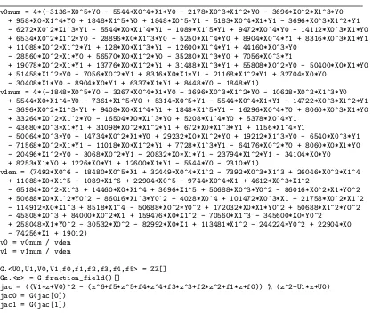
Figure 2.4.Together with Figure 2.5: Formulas for a rational mapι:W →J.
generalizes our example from Section 2.2. The Scholten curve is again y2=z6+ (7/3)z5−
(7/4)z4−(14/3)z3+ (7/4)z2+ (7/3)z−1 andω∈Fp2 satisfiesω2=−384.
The inputs toιare the coordinates (X0, X1, Y0, Y1) of a point (X0+X1i, ω(Y0+Y1i)) on the elliptic curve. The outputs are the Mumford coordinates (u0, u1, v0, v1) of a point onJ; recall that the affine part of J is defined by the equation (v1z+v0)2−f modz2+u1z+u0= 0. What the figures display is actually a Sage script verifying that (u0, u1, v0, v1) satisfies this equation. The script takes 25 seconds to run using Sage 6.1.1 on an Intel Xeon E3-1275 v3.
The exceptional cases of these formulas are not obvious without further calculation. One can see from the monomials appearing in the denominators that the denominators are not generically 0 over Z, but this does not rule out primes of bad reduction for which the denominators are always 0. We changedZ[i]/(i2+ 1) toF
p[i]/(i2+ 1) withp= 217−1, added
a check that the ideal of assumptions is prime, and ran the script again; this took 3 seconds. We then changed p to 2127−309, removed the primality check (since Sage’s tests for ideal primality use Singular and are limited to small characteristic), and ran the script again; this was vastly slower.
v0num = 4*(-3136*X0^5*Y0 - 5544*X0^4*X1*Y0 - 2178*X0^3*X1^2*Y0 - 3696*X0^2*X1^3*Y0 + 958*X0*X1^4*Y0 + 1848*X1^5*Y0 + 1848*X0^5*Y1 - 5183*X0^4*X1*Y1 - 3696*X0^3*X1^2*Y1 - 6272*X0^2*X1^3*Y1 - 5544*X0*X1^4*Y1 - 1089*X1^5*Y1 + 9472*X0^4*Y0 - 14112*X0^3*X1*Y0 + 6534*X0^2*X1^2*Y0 - 28896*X0*X1^3*Y0 + 5250*X1^4*Y0 + 8904*X0^4*Y1 + 8316*X0^3*X1*Y1 + 11088*X0^2*X1^2*Y1 + 128*X0*X1^3*Y1 - 12600*X1^4*Y1 + 44160*X0^3*Y0
- 28560*X0^2*X1*Y0 + 56570*X0*X1^2*Y0 - 35280*X1^3*Y0 + 7056*X0^3*Y1
+ 19078*X0^2*X1*Y1 + 13776*X0*X1^2*Y1 + 31488*X1^3*Y1 + 55808*X0^2*Y0 - 50400*X0*X1*Y0 + 51458*X1^2*Y0 - 7056*X0^2*Y1 + 8316*X0*X1*Y1 - 21168*X1^2*Y1 + 32704*X0*Y0
- 30408*X1*Y0 - 8904*X0*Y1 + 6337*X1*Y1 + 8448*Y0 - 1848*Y1)
v1num = 4*(-1848*X0^5*Y0 - 3267*X0^4*X1*Y0 + 3696*X0^3*X1^2*Y0 - 10628*X0^2*X1^3*Y0 + 5544*X0*X1^4*Y0 - 7361*X1^5*Y0 + 5314*X0^5*Y1 - 5544*X0^4*X1*Y1 + 14722*X0^3*X1^2*Y1 - 3696*X0^2*X1^3*Y1 + 9408*X0*X1^4*Y1 + 1848*X1^5*Y1 - 16296*X0^4*Y0 + 8060*X0^3*X1*Y0 + 33264*X0^2*X1^2*Y0 - 16504*X0*X1^3*Y0 + 5208*X1^4*Y0 + 5378*X0^4*Y1
- 43680*X0^3*X1*Y1 + 31098*X0^2*X1^2*Y1 + 672*X0*X1^3*Y1 + 1156*X1^4*Y1
- 50064*X0^3*Y0 + 14734*X0^2*X1*Y0 + 29232*X0*X1^2*Y0 + 19212*X1^3*Y0 - 6540*X0^3*Y1 - 71568*X0^2*X1*Y1 - 11018*X0*X1^2*Y1 + 7728*X1^3*Y1 - 64176*X0^2*Y0 + 8060*X0*X1*Y0 - 20496*X1^2*Y0 - 3068*X0^2*Y1 - 20832*X0*X1*Y1 - 23794*X1^2*Y1 - 34104*X0*Y0 + 8253*X1*Y0 + 1226*X0*Y1 + 12600*X1*Y1 - 5544*Y0 - 2310*Y1)
vden = (7492*X0^6 - 18480*X0^5*X1 + 32449*X0^4*X1^2 - 7392*X0^3*X1^3 + 26046*X0^2*X1^4 + 11088*X0*X1^5 + 1089*X1^6 + 22904*X0^5 - 9744*X0^4*X1 + 4612*X0^3*X1^2
- 65184*X0^2*X1^3 + 14460*X0*X1^4 + 3696*X1^5 + 50688*X0^3*Y0^2 - 86016*X0^2*X1*Y0^2 + 50688*X0*X1^2*Y0^2 - 86016*X1^3*Y0^2 + 4028*X0^4 + 101472*X0^3*X1 + 21758*X0^2*X1^2 - 114912*X0*X1^3 + 8518*X1^4 - 50688*X0^2*Y0^2 + 172032*X0*X1*Y0^2 + 50688*X1^2*Y0^2 - 45808*X0^3 + 84000*X0^2*X1 + 159476*X0*X1^2 - 70560*X1^3 - 345600*X0*Y0^2
+ 258048*X1*Y0^2 - 30532*X0^2 - 82992*X0*X1 + 113481*X1^2 - 244224*Y0^2 + 22904*X0 - 74256*X1 + 19012)
v0 = v0num / vden v1 = v1num / vden
G.<U0,U1,V0,V1,f0,f1,f2,f3,f4,f5> = ZZ[] Gz.<z> = G.fraction_field()[]
jac = ((V1*z+V0)^2 - (z^6+f5*z^5+f4*z^4+f3*z^3+f2*z^2+f1*z+f0)) % (z^2+U1*z+U0) jac0 = G(jac[0])
jac1 = G(jac[1])
thisjac0 = jac0(u0,u1,v0,v1,f[0],f[1],f[2],f[3],f[4],f[5]) thisjac1 = jac1(u0,u1,v0,v1,f[0],f[1],f[2],f[3],f[4],f[5]) print numerator(thisjac0) in assumptions
print numerator(thisjac1) in assumptions print not denominator(thisjac0) in assumptions print not denominator(thisjac1) in assumptions
Figure 2.5.Continuation of Figure 2.4.
p, any shape ofFp2, and any choices ofr, s, βin Section 2.1. Presumably a larger computation
along the same lines would produce a universal formula forι(with, e.g., the trace ofrappearing in the universal formula at the four positions where 66 appears as a coefficient in Figure 2.4), incidentally proving thatι does in fact exist in general, but what we actually need is merely the ability to findιfor whichever curves we decide to use in Section 1.
2.6. Explicitly mappingJ toW
R.<b,bp,r,rp,s,sp,u0,u1,v0,v1> = ZZ[] Rz.<z> = R[]
ww = r*bp^6+s*bp^4*b^2+sp*bp^2*b^4+rp*b^6
wwf = r*(1-bp*z)^6+s*(1-bp*z)^4*(1-b*z)^2+sp*(1-bp*z)^2*(1-b*z)^4+rp*(1-b*z)^6 jac = (ww*(v1*z+v0)^2 - wwf) % (z^2+u1*z+u0)
assumptions = (jac[0],jac[1])*R
bT = b+bp bN = b*bp
D = b^2*u0+b*u1+1
Z = (bp-b)*(2*bN*u0+bT*u1+2)*D
Lw = (b^3*(u0*v0+u0*u1*v1-u1^2*v0)+3*b^2*(u0*v1-u1*v0)-3*b*v0-v1)/Z # implicitly: L = w*Lw
F = 2*bN^2*u0^2+2*bN*bT*u0*u1+(b^2+bp^2)*u1^2-2*(b^2+bp^2-4*bN)*u0+2*bT*u1+2 X = (ww*Lw^2-s)/r - F/D^2
Yw = (bN*bp*(u0*v0+u0*u1*v1-u1^2*v0)+bp*(b+bT)*(u0*v1-u1*v0)-(bp+bT)*v0-v1)/Z-Lw*X # implicitly: Y = w*Yw
curve = r*X^3+s*X^2+sp*X+rp-ww*Yw^2 denom = r*Z^6
print R(denom*curve) in assumptions print not denom in assumptions
Figure 2.7.Formulas for a rational mapι0:J→W.
P, Q, P+Q∈W(Fp) then they produce ι(P), ι(Q), ι(P+Q) =ι(P) +ι(Q) respectively in
J(Fp). One can directly prove this fact by a straightforward computation without any reference
to the theory of isogenies. If we were applying ι to non-random inputs then we would need a complete system of formulas, supplementing our rational functions with further formulas to handle exceptional cases.
Figure 2.7 exhibits formulas for ι0. These formulas are stated in more generality than our formulas forι: they apply to all of the curves reviewed in Section 2.1. Section 3 explains how we computed these formulas. The inputs toι0 are Mumford coordinates (u0, u1, v0, v1) for a point on J, and the outputs are four coordinates for a point on W. The script actually produces (X, Y) using arithmetic overFp2 and verifies that (X, Y) satisfies the curve equation for E;
there is no need to give separate names to the fourW coordinates that correspond to (X, Y). The script takes 170 seconds to run.
The exceptional cases of these formulas are clear from inspection, since all denominators are given in factored form as products of constants and linear functions. Specifically, there are divisions byβ2u
0+βu1+ 1, by 2ββpu0+ (βp+β)u1+ 2, and by the nonzero constantsrand βp−β.
Figure 2.8 is a Sage script verifying that applyingιto a generic pointP onW, andι0to the result, produces exactly 2P. The script takes 78 seconds forp= 217−1; it is much slower for p= 2127−309 and for Z.
p = 2^17-1
# p = 0 for generic
if p: R1 = GF(p) P1.<polyi> = R1[]
R2.<i> = GF(p^2,name=’i’,modulus=polyi^2+1) else:
R1 = ZZ
P1.<polyi> = R1[]
R2.<i> = P1.quotient(polyi^2+1)
r,s,b = 33+56*i,159+56*i,i rp,sp,bp = 33-56*i,159-56*i,-i
ww = R1(r*bp^6+s*bp^4*b^2+sp*bp^2*b^4+rp*b^6) R2z.<z> = R2[]
wwf = r*(1-bp*z)^6+s*(1-bp*z)^4*(1-b*z)^2+sp*(1-bp*z)^2*(1-b*z)^4+rp*(1-b*z)^6 f = wwf.change_ring(R1) / ww
P2.<X0,X1,Y0,Y1> = R2[] X = X0+X1*i
Yw = Y0+Y1*i
curve = r*X^3+s*X^2+sp*X+rp-ww*Yw^2 if p:
curvereal = curve.map_coefficients(lambda u:u.polynomial()[0]) curveimag = curve.map_coefficients(lambda u:u.polynomial()[1]) else:
curvereal = curve.map_coefficients(lambda u:u[0]) curveimag = curve.map_coefficients(lambda u:u[1]) assumptions = (curvereal,curveimag)*P2
if p > 0 and p < 2^20: # unimplemented for large p in Sage (via Singular) print assumptions.is_prime()
# Weierstrass doubling: Xorig = X
Yworig = Yw
la = (3*r*Xorig^2+2*s*Xorig+sp)/(2*ww*Yworig) Xdbl = (ww*la^2-s)/r - 2*Xorig
Ywdbl = la*(Xorig-Xdbl) - Yworig
# isogeny from W to J:
u0num = (240*X0^3*Y0 + 1787*X0^2*X1*Y0 - 1248*X0*X1^2*Y0 - 297*X1^3*Y0 - 224*X0^3*Y1 + 612*X0^2*X1*Y1 + 1860*X0*X1^2*Y1 - 876*X1^3*Y1 + 2862*X0*X1*Y0 - 1952*X0^2*Y1 + 744*X0*X1*Y1 + 1952*X1^2*Y1 - 240*X0*Y0 + 535*X1*Y0 - 3232*X0*Y1 + 372*X1*Y1 - 1504*Y1)
u0den = (504*X0^3*Y0 + 1339*X0^2*X1*Y0 - 984*X0*X1^2*Y0 - 745*X1^3*Y0 - 818*X0^3*Y1 + 1620*X0^2*X1*Y1 + 1266*X0*X1^2*Y1 + 132*X1^3*Y1 - 264*X0^2*Y0 + 3758*X0*X1*Y0 + 264*X1^2*Y0 - 1358*X0^2*Y1 - 1272*X0*X1*Y1 + 1358*X1^2*Y1 - 2040*X0*Y0 + 1879*X1*Y0 + 818*X0*Y1 - 2652*X1*Y1 - 1272*Y0 + 1358*Y1)
u1num = 2*Y1*(-56*X0^3 - 33*X0^2*X1 - 56*X0*X1^2 - 33*X1^3 - 56*X0^2 - 66*X0*X1 + 56*X1^2 + 56*X0 - 93*X1 + 56)
Figure 2.8.Together with Figure 2.9: Verification that doubling onW matches the composition of ι0:J→W andι:W →J.
3. Finding efficient isogenies
u1den = (56*X0^3*Y0 + 99*X0^2*X1*Y0 - 168*X0*X1^2*Y0 - 33*X1^3*Y0 - 66*X0^3*Y1 + 224*X0^2*X1*Y1 + 66*X0*X1^2*Y1 + 56*X0^2*Y0 + 318*X0*X1*Y0 - 56*X1^2*Y0 - 126*X0^2*Y1 + 126*X1^2*Y1 - 56*X0*Y0 + 159*X1*Y0 + 66*X0*Y1 - 224*X1*Y1 - 56*Y0 + 126*Y1)
u0 = u0num / u0den u1 = u1num / u1den
v0num = 4*(-3136*X0^5*Y0 - 5544*X0^4*X1*Y0 - 2178*X0^3*X1^2*Y0 - 3696*X0^2*X1^3*Y0 + 958*X0*X1^4*Y0 + 1848*X1^5*Y0 + 1848*X0^5*Y1 - 5183*X0^4*X1*Y1 - 3696*X0^3*X1^2*Y1 - 6272*X0^2*X1^3*Y1 - 5544*X0*X1^4*Y1 - 1089*X1^5*Y1 + 9472*X0^4*Y0 - 14112*X0^3*X1*Y0 + 6534*X0^2*X1^2*Y0 - 28896*X0*X1^3*Y0 + 5250*X1^4*Y0 + 8904*X0^4*Y1 + 8316*X0^3*X1*Y1 + 11088*X0^2*X1^2*Y1 + 128*X0*X1^3*Y1 - 12600*X1^4*Y1 + 44160*X0^3*Y0
- 28560*X0^2*X1*Y0 + 56570*X0*X1^2*Y0 - 35280*X1^3*Y0 + 7056*X0^3*Y1
+ 19078*X0^2*X1*Y1 + 13776*X0*X1^2*Y1 + 31488*X1^3*Y1 + 55808*X0^2*Y0 - 50400*X0*X1*Y0 + 51458*X1^2*Y0 - 7056*X0^2*Y1 + 8316*X0*X1*Y1 - 21168*X1^2*Y1 + 32704*X0*Y0
- 30408*X1*Y0 - 8904*X0*Y1 + 6337*X1*Y1 + 8448*Y0 - 1848*Y1)
v1num = 4*(-1848*X0^5*Y0 - 3267*X0^4*X1*Y0 + 3696*X0^3*X1^2*Y0 - 10628*X0^2*X1^3*Y0 + 5544*X0*X1^4*Y0 - 7361*X1^5*Y0 + 5314*X0^5*Y1 - 5544*X0^4*X1*Y1 + 14722*X0^3*X1^2*Y1 - 3696*X0^2*X1^3*Y1 + 9408*X0*X1^4*Y1 + 1848*X1^5*Y1 - 16296*X0^4*Y0 + 8060*X0^3*X1*Y0 + 33264*X0^2*X1^2*Y0 - 16504*X0*X1^3*Y0 + 5208*X1^4*Y0 + 5378*X0^4*Y1
- 43680*X0^3*X1*Y1 + 31098*X0^2*X1^2*Y1 + 672*X0*X1^3*Y1 + 1156*X1^4*Y1
- 50064*X0^3*Y0 + 14734*X0^2*X1*Y0 + 29232*X0*X1^2*Y0 + 19212*X1^3*Y0 - 6540*X0^3*Y1 - 71568*X0^2*X1*Y1 - 11018*X0*X1^2*Y1 + 7728*X1^3*Y1 - 64176*X0^2*Y0 + 8060*X0*X1*Y0 - 20496*X1^2*Y0 - 3068*X0^2*Y1 - 20832*X0*X1*Y1 - 23794*X1^2*Y1 - 34104*X0*Y0 + 8253*X1*Y0 + 1226*X0*Y1 + 12600*X1*Y1 - 5544*Y0 - 2310*Y1)
vden = (7492*X0^6 - 18480*X0^5*X1 + 32449*X0^4*X1^2 - 7392*X0^3*X1^3 + 26046*X0^2*X1^4 + 11088*X0*X1^5 + 1089*X1^6 + 22904*X0^5 - 9744*X0^4*X1 + 4612*X0^3*X1^2
- 65184*X0^2*X1^3 + 14460*X0*X1^4 + 3696*X1^5 + 50688*X0^3*Y0^2 - 86016*X0^2*X1*Y0^2 + 50688*X0*X1^2*Y0^2 - 86016*X1^3*Y0^2 + 4028*X0^4 + 101472*X0^3*X1 + 21758*X0^2*X1^2 - 114912*X0*X1^3 + 8518*X1^4 - 50688*X0^2*Y0^2 + 172032*X0*X1*Y0^2 + 50688*X1^2*Y0^2 - 45808*X0^3 + 84000*X0^2*X1 + 159476*X0*X1^2 - 70560*X1^3 - 345600*X0*Y0^2
+ 258048*X1*Y0^2 - 30532*X0^2 - 82992*X0*X1 + 113481*X1^2 - 244224*Y0^2 + 22904*X0 - 74256*X1 + 19012)
v0 = v0num / vden v1 = v1num / vden
# isogeny from J to W: bT = b+bp
bN = b*bp
D = b^2*u0+b*u1+1
Z = (bp-b)*(2*bN*u0+bT*u1+2)*D
Lw = (b^3*(u0*v0+u0*u1*v1-u1^2*v0)+3*b^2*(u0*v1-u1*v0)-3*b*v0-v1)/Z
F = 2*bN^2*u0^2+2*bN*bT*u0*u1+(b^2+bp^2)*u1^2-2*(b^2+bp^2-4*bN)*u0+2*bT*u1+2 X = (ww*Lw^2-s)/r - F/D^2
Yw = (bN*bp*(u0*v0+u0*u1*v1-u1^2*v0)+bp*(b+bT)*(u0*v1-u1*v0)-(bp+bT)*v0-v1)/Z-Lw*X
Xequal = X - Xdbl Ywequal = Yw - Ywdbl
print numerator(Xequal) in assumptions print numerator(Ywequal) in assumptions print not denominator(Xequal) in assumptions print not denominator(Ywequal) in assumptions
Figure 2.9.Continuation of Figure 2.8.
3.1. The covering map
Define a rational map φfrom the hyperelliptic curveH :y2=f(z) to the elliptic curve E: y2=rx3+sx2+spx+rp, namelyφ(z, y) = (x2, ωy/(1−βz)3) wherex= (1−βpz)/(1−βz). To see that this works, observe that ω2f(z)/(1−βz)6=rx6+sx4+spx2+rp by definition off. The map φ, modulo notation, appeared in Scholten’s proof of [48, Lemma 2.1].
Next define a rational mapφ2fromH×H toW as follows: map (P1, P2) to the sumφ(P1) + φ(P2) onE, and then to the coordinates of the sum in W. These coordinates are symmetric betweenP1 andP2, soφ2 must factor as a composition of the standard mapH×H →J and some rational mapι0 :J →W.
Of course, a rational map from J to W is not necessarily an isogeny. The map might shift 0 to something nonzero (which would not be a disaster for us), or it might lose one or two dimensions (which would be a disaster). On the other hand, it is at least intuitively clear that 0 maps to 0, sinceφ(z,−y) =−φ(z, y). Furthermore, if #E(Fp2) has a large prime divisor (not
far below p2), as often happens, then one expects a “random” size-p subset S of E(F
p2) to
haveS+Scovering a considerable fraction ofE(Fp2), while any drop of dimension would make
#ι0(J(Fp)) much smaller than #W(Fp) = #E(Fp2) for largep. Not all subsets are “random”
(for example,pconsecutive multiples of a generator have only 2p−1 sums), but the algebraic constraints onφ(H) seem unlikely to produce such behavior. So it is reasonable to hope that ι0 is an isogeny.
3.2. The hard approach
At this point the conventional analysis of isogenies would continue by carrying out various time-consuming computations:
• Prove thatι0 really is an isogeny. The main work here is analyzing the fibers ofι0 via the fibers of φ2.
• Deduce that, for various positive integers d, multiplication by don W can be expressed as ι0◦ι, and multiplication by d on J can be expressed as ι◦ι0, where ι is an isogeny. Figure out the smallest possible d by comparing the structure of the fibers of ι0 to the group structure ofJ.
• Compute explicit formulas for ι0 as follows. Start with generic points P1= (z1, y1) and P2= (z2, y2) onH, i.e., the points (z1, y1) and (z2, y2) onH overFp(z1, z2)[y1, y2]/(y21− f(z1), y22−f(z2)). Compose the definition ofφwith the addition formulas onEto obtain φ(P1) +φ(P2) as explicit rational functions inz1, z2, y1, y2. Eliminatez1, z2, y1, y2 in favor of the Mumford coordinatesu0=z1z2,u1=−z1−z2,v1= (y2−y1)/(z2−z1),v0=y1− v1z1.
• Observe that these explicit formulas forι0involve many terms. Search for simpler formulas,
presumably accelerating evaluation ofι0 and also accelerating the rest of the analysis, by
strategically exploiting equations satisfied by the Mumford coordinates. See [42] for a systematic “rational simplification” algorithm; see [30] for the first use of this algorithm to simplify elliptic-curve formulas.
• View d(u0, u1, v0, v1) =ι(ι0(u0, u1, v0, v1)), or the analogous equation onW, as a system of equations for the dual isogeny ι. Solve these equations somehow.
One could carry out this type of analysis for specific choices of the parameters p, r, s, β, obtaining formulas for ι0 and ι for those parameters, which is what we actually need. Alternatively, with more computation, one could leave the parameters as variables, obtaining general formulas forι0 andιand then specializing the formulas upon demand.
exactlyι, and d= 2. One can obtain explicit formulas for this map from explicit formulas for addition onJ, and one can then search for simpler formulas as above.
3.3. The easy approach
We take a different, much easier, approach to compute formulas for ι0. We fix parameters, takerandompoints (z1, y1),(z2, y2)∈H(Fp), compute the corresponding Mumford coordinates
u0, u1, v0, v1 in Fp (skipping the degenerate case z1=z2), and compute φ(z1, y1) +φ(z2, y2) as two coordinates in Fp2, i.e., four coordinates in Fp. This computation tells us a specific
value of ι0 for a specific input (u0, u1, v0, v1); this linearly constrains the coefficients in the numerator and denominator of each coordinate of ι0. Taking more random points gives us more linear constraints. For each coordinate we guess a limit on the degree (or a more refined set of monomials) for the smallest possible numerator and denominator; take significantly more points than monomials; and solve the resulting system of linear equations. If there are enough points then all nonzero solutions will define the same rational map, and if the guess was correct then this rational map must beι0.
The same idea easily producesι. We start by guessing thatd= 2 will work, i.e., that we will be able to findιwith 2(u0, u1, v0, v1) =ι(ι0(u0, u1, v0, v1)). For random points (z1, y1),(z2, y2)∈ H(Fp), we compute (u0, u1, v0, v1) andι0(u0, u1, v0, v1) as above, and also double (u0, u1, v0, v1)
onJ (skipping degenerate cases) to obtain 2(u0, u1, v0, v1). This tells us an input-output pair forι, and thus linearly constrains the coefficients in the numerator and denominator of each coordinate ofι.
Of course, this does notprove that the formulas that we obtain are the same as theι0 and
ιdefined in this section. It is conceivable that our formulas were amazingly lucky, matchingι0 andιon many random points, while the realι0 andιescaped detection by requiring monomials of higher degree than the monomials in our computation. One response is that, having verified (see Section 2.6) that our formulas are in fact efficient dual isogenies, we can simply use these formulas, and no longer need this section’s definition of a possibly different function ι0. A different response is to verify symbolically that the functions are in fact the same. Figure 3.4 does exactly this; the script takes 24 seconds to run.
The interpolation strategy described in this section can be viewed as a way to simplify formulas forι0 (andι). We emphasize, however, that the input to interpolation does not need to be aformulaforι0; it can be any method ofcomputingenough input-output pairs forι0. This is what lets us skip all of the intermediate computations inFp(z1, z2)[y1, y2]/(y12−f(z1), y
2 2− f(z2)). We also comment that, even though all we need is to be able to compute ι0 and ι efficiently for specific curve parameters, one can also interpolate generic formulas that work for arbitrary parameters. This is what we did forι0, producing the extra generality of Figure 2.7 compared to Figures 2.4 and 2.5.
We actually deviated slightly from the strategy stated above: rather than interpolating formulas forι0, we interpolated formulas for certain intermediate results that obviously play an important role inι0 and that remain visible in Figure 2.7. Specifically,F/D2=x2
1+x22 where xi= (1−βpzi)/(1−βzi), andLis the slope in the usual Weierstrass-curve addition formulas.
4. Jacobian to Kummer
In Section 2 we constructed efficient isogenies between W and J, where W is the Weil restriction of an elliptic curve fromFp2 toFp and J is the Jacobian of a hyperelliptic curve
y2=f(z) in Scholten form overFp.
We now restrict the choice of hyperelliptic curve to improve the efficiency of scalar multiplication inJ(Fp). Specifically, in this section, we force the corresponding Kummer surface
R.<r,s,w,b,bp,u0,u1,v0,v1,z1,z2,y1,y2> = ZZ[]
assumptions = (u0-z1*z2,u1+z1+z2,v1*(z1-z2)-(y1-y2),y1-v1*z1-v0)*R
x1 = (1-bp*z1)/(1-b*z1) x2 = (1-bp*z2)/(1-b*z2) sumxin = r*x1^2+r*x2^2
la = (r*w*y1/(1-b*z1)^3-r*w*y2/(1-b*z2)^3)/(r*x1^2-r*x2^2) x3 = (la^2-s-sumxin)/r
y3 = la*(x1^2-x3)-w*y1/(1-b*z1)^3
ww = w*w bT = b+bp bN = b*bp
D = b^2*u0+b*u1+1
Z = (bp-b)*(2*bN*u0+bT*u1+2)*D
Lw = (b^3*(u0*v0+u0*u1*v1-u1^2*v0)+3*b^2*(u0*v1-u1*v0)-3*b*v0-v1)/Z L = w*Lw
F = 2*bN^2*u0^2+2*bN*bT*u0*u1+(b^2+bp^2)*u1^2-2*(b^2+bp^2-4*bN)*u0+2*bT*u1+2 X = (ww*Lw^2-s)/r - F/D^2
Yw = (bN*bp*(u0*v0+u0*u1*v1-u1^2*v0)+bp*(b+bT)*(u0*v1-u1*v0)-(bp+bT)*v0-v1)/Z-Lw*X Y = w*Yw
denom = Z*(z2-z1)*(bp-b)*(1-b*z2)*(1-b*z1)*(2*b*bp*z1*z2-(b+bp)*(z1+z2)+2) print R(denom*(la-L)) in assumptions
print R(denom^2*(sumxin-r*F/D^2)) in assumptions print R(r*denom^2*(x3-X)) in assumptions
check = r*denom^3*y3-r*denom^3*Y # R(check) segfaults
print denominator(check) == 1
print R(numerator(check)) in assumptions print not r*denom^3 in assumptions
Figure 3.4.Verification that the formulas in Figure 2.7 map a generic element ofJwith affine part (P1) + (P2)toφ(P1) +φ(P2).
Gaudry’s highly efficient formulas for the action ofZon theZ-setK(Fp), i.e., for the standard
scalar-multiplication functionZ×K(Fp)→K(Fp). See Section 6 for further curve constraints
that save time inside Gaudry’s formulas.
4.1. Constraints onf
We reject Scholten’s sextic polynomial f unless it splits completely over Fp. Rather than
testing this we constructf in a way that enforces it; see Section 4.2.
Once we have an f that splits, we convert the Scholten curve to twisted Rosenhain form δy2=x(x−1)(x−λ)(x−µ)(x−ν) overF
p, by definingzas a linear fractional transformation
of xthat moves three roots of f in z to 0,1,∞ in x. This transformation of curves induces a transformation of the Jacobians. Note that there are many choices of three roots and thus many choices of Rosenhain curve.
We then obtain the Kummer surface corresponding to (λ, µ, ν) as in [6, full version, Section 5.2]: compute d2= 1, c2=±p
λµ/ν, b2=p
µ(µ−1)(λ−ν)/(ν(ν−1)(λ−µ)), and a2=b2c2ν/µ. We reject (λ, µ, ν) if these two square roots are not in Fp. Note that there are
six choices of (λ, µ, ν) for each Rosenhain curve.
We also check the “genericity conditions” hypothesized by [25]. Specifically, we check that the quantities a2d2−b2c2, a2c2−b2d2, a2b2−c2d2, A2=a2+b2+c2+d2, B2=a2+b2− c2−d2, C2=a2−b2+c2−d2, D2=a2−b2−c2+d2 are nonzero. This ensures that the denominators are nonzero in the quantitiesE, F, G, H appearing below. (The conditions stated in [25] are thatA, B, C, Dare nonzero and that various theta constantsθ5, θ6, θ7, θ8, θ9, θ10are all nonzero when (θ1:θ2:θ3:θ4) = (a:b:c:d). The formula θ52θ26=θ12θ42−θ22θ23 shows that ifθ5= 0 or θ6= 0 then a2d2−b2c2= 0; similar comments apply to θ72θ29=θ21θ23−θ22θ42 and θ2
8θ210=θ12θ22−θ23θ24.)
Beware that the reverse formulas forλ, µ, νin terms ofa, b, c, d, A, B, C, Din [6, full version, Section 5.2] are correct for our definitions of A, B, C, D but incorrect for the definitions of A, B, C, Din [6]. Further warnings regarding formulas in the literature appear in Section 4.4. This procedure forces J to have full 2-torsion. Consequently the group order #J(Fp) is
divisible by 16. For cryptographic purposes we need a large prime in the group order; we restrict attention to the simplest case, namely groups of order 16` where ` is a large prime. Our numerical example in Section 2.2 shows that this case does occur; we return to this example in Section 4.3.
4.2. Scholten Jacobians with full2-torsion
By hypothesis y2=rx3+sx2+spx+rp is elliptic. Consequently r6= 0, and the cubic
rx3+sx2+spx+rp factors over an extension ofF
p as r(x−ρ1)(x−ρ2)(x−ρ3) for distinct ρ1, ρ2, ρ3. The product−rρ1ρ2ρ3equalsrpso all ofρ1, ρ2, ρ3are nonzero. Choose a square root √
ρj of eachρj in a suitable extension ofFp.
Now assume that the Jacobian of Scholten’s hyperelliptic curve has full 2-torsion defined overFp, i.e., that there are 6 distinct roots inFp of the degree-6 polynomial
r(1−βpz)6+s(1−βpz)4(1−βz)2+sp(1−βpz)2(1−βz)4+rp(1−βz)6
=r((1−βpz)2−ρ1(1−βz)2)((1−βpz)2−ρ2(1−βz)2)((1−βpz)2−ρ3(1−βz)2).
This polynomial visibly splits into linear factors of the form (1−βpz±√ρj(1−βz)), so each
(1±√ρj)/(βp±β √
ρj) must be inFp; in other words, each √
ρj has the form (1−βpζ)/(1−
βζ) for some ζ∈Fp. This implies √
ρj∈Fp2 and
√
ρjp= (1−βζ)/(1−βpζ) = 1/ √
ρj; i.e.,
each√ρj has norm 1.
Conversely, take any three norm-1 elements√ρ1,√ρ2,√ρ3∈Fp2 with distinct squares. The
product−ρ1ρ2ρ3has norm 1 and thus can be written asrp/rfor somer∈F∗p2, for example for
r=i(√ρ1 √
ρ2 √
ρ3)p. Defines=−r(ρ1+ρ2+ρ3); thenrx3+sx2+spx+rp=r(x−ρ1)(x− ρ2)(x−ρ3) soy2=rx3+sx2+spx+rpis elliptic. Choose anyβ∈Fp2 such thatβ /∈Fp and
βp−16=±√ρ
j. The ratio (1± √
ρj)/(βp±β √
ρj) has conjugate (1±1/ √
ρj)/(β±βp/ √
ρj) =
(√ρj±1)/(β √
ρj±βp) = (1± √
ρj)/(βp±β √
ρj) and is thus inFp. There are six such ratios,
all distinct since z7→(1−βpz)/(1−βz) maps them to ±√ρ
j, and each of these ratios is a
root of Scholten’s degree-6 polynomial.
4.3. A numerical example, continued
As a generalization of the example in Section 2.2, takep∈3 + 4ZwithFp2 =Fp[i]/(i2+ 1),
assume p >13, and take √ρ1=i, √ρ2= (3 + 4i)/5, and √ρ3= (5 + 12i)/13. The product
−ρ1ρ2ρ3=−(2047 + 3696i)/4225 then has the form rp/r for, e.g., r= 33 + 56i. Define s=
This structure forces the polynomial f in Section 2.2 to split over Fp: specifically, z6+
(7/3)z5−(7/4)z4−(14/3)z3+ (7/4)z2+ (7/3)z−1 has roots 1 and −1 via √ρ1, roots 1/2 and−2 via√ρ2, and roots 2/3 and−3/2 via√ρ3.
The linear fractional transformation z7→5(1−z)/(2 +z) takes 1,1/2,−2,−1,2/3,−3/2 to 0,1,∞, λ, µ, ν respectively, where λ= 10, µ= 5/8, ν= 25. The ratio λµ/ν is a square, namely 1/22, and the ratio µ(µ−1)(λ−ν)/(ν(ν−1)(λ−µ)) is a square, namely 1/402. Taking positive signs for the square roots produces (a2, b2, c2, d2) = (1/2,1/40,1/2,1) and (A2, B2, C2, D2) = (81/40,−39/40,−1/40,39/40); we scale these to (20,1,20,40) and (81,−39,−1,39) respectively. The differencesa2b2−c2d2,a2c2−b2d2,a2d2−b2c2are nonzero.
4.4. Explicit maps from the Jacobian to the Kummer surface
It is not easy to find correct formulas in the literature for the standard rational map from a JacobianJ of a genus-2 hyperelliptic curve to a Kummer surfaceK. The conventional view arises from expressingJ (in Mumford coordinates) and K (a particular quartic surface with various symmetries) in terms of 16 different Riemann theta functions and then solving for the coordinates of one in terms of the other; but this involves a huge thicket of theta formulas, with many opportunities for errors. For example:
• The formula for θ47+θ94in [25, page 262] is incorrect: it needs to be negated.
• The formula for v20 in [12, page 1206] is incorrect: the second minus sign needs to be a plus, as pointed out in [6].
• The definitions of A, B, C, D in [6, Section 5.1] are incorrect for the stated parameter relationship between J andK: they need to be replaced byA2, B2, C2, D2. On the other hand, the definitions are consistent with some other formulas in [6], so those other formulas also need to be modified.
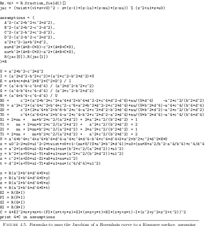
We need to actually compute this map, rather than merely to write papers about it, so we need correct formulas. To avoid errors we present in Figure 4.5 a Sage script verifying our formulas for this map. We have also put considerable effort into simplifying these formulas, eliminating unnecessary detours through theta functions. The script takes 70 seconds to run, and the formulas have bad reduction only at 2.
Computer-algebra scripts for “Kummer surface” formulas have been published before: see the web site [20] accompanying the book [10] by Cassels and Flynn. However, the “Kummer surface”K0 in [10] and [20] is much less efficient than the highly symmetric Kummer surface K used in [11], [25], [12], [6], [4], and this paper. (We question the use of the terminology “Kummer surface” forK0; we speculate that Kummer would have been horrified to have his name attached toK0.) BothKandK0 are isomorphic toJ/{±1}and therefore to each other,
but the choice of coordinates is critical for performance, and there is no reason to think that finding formulas for this isomorphism fromK0 toK would be easier than finding formulas for the map fromJ toK.
Our script starts with a generic point (u0, u1, v0, v1) in Mumford coordinates on the Jacobian of a twisted Rosenhain curveδY2=X(X−1)(X−λ)(X−µ)(X−ν) with 0,1, λ, µ, νdistinct. Recall, as in Section 2, that the affine part of the Jacobian is defined by the equation
δ(v1X+v0)2−X(X−1)(X−λ)(X−µ)(X−ν) modX2+u1X+u0= 0.
The script computes particular linear combinationsx, y, z, tofu20, u0u21, v0v1, u0,1, u1, u0u1, u21, and verifies that (x:y:z:t) satisfies the Kummer-surface equation
assuming certain relationships between the Kummer-surface parameters E, F, G, H and the Rosenhain-curve parametersλ, µ, ν. The assumptions are
λ=b 2d2
a2c2, F =
a4−b4−c4+d4 a2d2−b2c2 , A
2=a2+b2+c2+d2,
µ= c
2(AB+CD)
d2(AB−CD), G=
a4−b4+c4−d4 a2c2−b2d2 , B
2=a2+b2−c2−d2,
ν =a
2(AB+CD)
b2(AB−CD), H =
a4+b4−c4−d4 a2b2−c2d2 , C
2=a2−b2+c2−d2,
E= abcdA
2B2C2D2
(a2d2−b2c2)(a2c2−b2d2)(a2b2−c2d2), D 2
=a2−b2−c2+d2.
The formulas above were typed by hand; readers are encouraged to instead consult Figure 4.5 for the original computer-verified formulas, including the details of the linear combinations.
Since the map does not usev0andv1except asv0v1, it does not distinguish−(u0, u1, v0, v1) = (u0, u1,−v0,−v1) from (u0, u1, v0, v1). With more work one can verify that a generic output point (x:y:z:t) has exactly two preimages, but we do not actually need this fact. For example, it would not be a problem if the map were actually doubling on J followed by the standard map fromJ/{±1}toK, since this would still act as a nonzeroZ-set morphism from the order-` subgroup of J(Fp) to the corresponding subset of K(Fp). Given any particular
curve we check that a generator of the order-`subgroup maps to a nonzero element ofK(Fp).
4.6. Explicit maps from the Kummer surface to the Jacobian
We do not report similarly optimized computer-verified formulas for computing preimages of the map in Figure 4.5. These preimages are not needed in Section 1. However, we briefly comment on such computations for applications that might need them.
A rational map cannot compute the preimages in J for a given element of K: the choice between two preimages is determined by a sign choice in a square root. This square root is, however, unnecessary for an application that actually wants to computeP 7→nP onJ. There is a rational map that producesnP inJ givenP inJ and the images ofnP,(n+ 1)P in K, and Gaudry’s formulas naturally compute (n+ 1)P for free while computingnP. See [43] for the analogous genus-1 case.
5. Weierstrass to Edwards: genus-1 efficiency and simplicity
Recall from Section 4 that we construct a group J(Fp) having order 16` where` is a large
prime. This also forces the group W(Fp) =E(Fp2) to have order 16`. This in turn forces
E(Fp2) to have at least one point of order 4, and thus to be expressible as an Edwards curve.
Computer experiments suggest that this procedure actually forces the order-16 subgroup of E(Fp2) to have shape (Z/4)×(Z/4), which we do not consider optimal, but in a moment we
will force the shape to be what we actually want.
To simplify elliptic-curve arithmetic we apply further 2-isogenies to obtain a complete
R.<u0,u1,v0,v1,la,mu,nu,A,B,C,D,a,b,c,d,twist> = ZZ[] Rz.<z> = R.fraction_field()[]
jac = (twist*(v1*z+v0)^2 - z*(z-1)*(z-la)*(z-mu)*(z-nu)) % (z^2+u1*z+u0)
assumptions = (
A^2-(a^2+b^2+c^2+d^2), B^2-(a^2+b^2-c^2-d^2), C^2-(a^2-b^2+c^2-d^2), D^2-(a^2-b^2-c^2+d^2), a^2*c^2-la*b^2*d^2,
mu*d^2*(A*B-C*D)-c^2*(A*B+C*D), nu*b^2*(A*B-C*D)-a^2*(A*B+C*D), R(jac[0]),R(jac[1])
)*R
U = a^2*b^2-c^2*d^2
I = (a^2*d^2-b^2*c^2)*(a^2*c^2-b^2*d^2)*U E = a*b*c*d*A^2*B^2*C^2*D^2 / I
F = (a^4-b^4-c^4+d^4) / (a^2*d^2-b^2*c^2) G = (a^4-b^4+c^4-d^4) / (a^2*c^2-b^2*d^2) H = (a^4+b^4-c^4-d^4) / U
X0 = c^2*(a^2*b^2*c^2+a^4*d^2+b^4*d^2-2*c^4*d^2-d^6)*nu/(U*d^4) -a^2*c^2/(b^2*d^2) Y0 = a^2*c^2*(a^4*c^2+b^4*c^2-c^6+a^2*b^2*d^2-2*c^2*d^4)*nu/(U*b^2*d^4)-a^4*c^4/(b^4*d^4) Z0 = c^2*(2*a^4*b^2+b^6-b^2*c^4-a^2*c^2*d^2-b^2*d^4)*nu/(U*b^2*d^2)-a^2*c^2/(b^2*d^2) T0 = c^4*(a^6+2*a^2*b^4-a^2*c^4-b^2*c^2*d^2-a^2*d^4)*nu/(U*b^2*d^4)-a^4*c^4/(b^4*d^4) X1 = 2*nu + nu*b^2*c^2/(a^2*d^2) + 2*a^2*c^2/(b^2*d^2) + 1
Y1 = nu + 2*nu*b^2*c^2/(a^2*d^2) + a^2*c^2/(b^2*d^2) + 2 Z1 = nu + 2*nu*b^2*c^2/(a^2*d^2) + 2*a^2*c^2/(b^2*d^2) + 1 T1 = 2*nu + nu*b^2*c^2/(a^2*d^2) + a^2*c^2/(b^2*d^2) + 2
V = a^4*b^4*c^4+a^4*b^4*d^4-a^4*c^4*d^4-b^4*c^4*d^4+2*a^2*b^2*c^2*d^2*H*U
s = u0^2-2*u0*u1^2-2*twist*v0*v1-(nu*V/(U*a^2*b^2*d^4))*u0+(nu*H*a^2/b^2-a^4/b^4)*c^4/d^4 x = a^2*(s+X0*u1-X1*u0*u1+nu*(b^2*c^2/(a^2*d^2))*u1^2)
y = b^2*(s+Y0*u1-Y1*u0*u1+nu*(a^2*c^2/(b^2*d^2))*u1^2) z = c^2*(s+Z0*u1-Z1*u0*u1+nu*u1^2)
t = d^2*(s+T0*u1-T1*u0*u1+nu*(c^4/d^4)*u1^2)
x = R(a^2*b^4*d^4*U*x) y = R(a^2*b^4*d^4*U*y) z = R(a^2*b^4*d^4*U*z) t = R(a^2*b^4*d^4*U*t) EI = R(E*I)
FI = R(F*I) GI = R(G*I) HI = R(H*I)
C = 4*EI^2*x*y*z*t-(FI*(x*t+y*z)+GI*(x*z+y*t)+HI*(x*y+z*t)-I*(x^2+y^2+z^2+t^2))^2 print 4*C in assumptions
Figure 4.5.Formulas to map the Jacobian of a Rosenhain curve to a Kummer surface, assuming certain relationships between the surface parameters and the curve parameters.
In the example below we use a chain of two 2-isogenies followed by the birational equivalence. These isogenies replace (Z/4)×(Z/4) first with (Z/8)×(Z/2) and then with Z/16. For background on the underlying “volcano” structure see, e.g., [50].
5.1. A numerical example, part III
Consider again the example in Section 2.2, withp= 2127−309,i2=−1,r= 33 + 56i, and s= 159 + 56i. We convert the elliptic curvey2=rx3+sx2+spx+rpoverFp2 to a complete
Substitute y= ¯y/r and x= ¯x/r, obtaining the isomorphic curve ¯y2= ¯x3+sx¯2+rspx¯+
r2rp, i.e., ¯y2= (¯x+ (63 + 16i))(¯x+ (63−16i))(¯x+ (33 + 56i)).
Substitute ¯y=y and ¯x=x−63−16i, obtaining y2=x(x−32i)(x−30 + 40i). Apply the standard 2-isogeny to ¯y2= ¯x3+ (60−16i)¯x2+ (−4284−4320i)¯x, which (for p= 2127−309) factors as ¯y2= ¯x(¯x−s1)(¯x−s2) wheres1, s2 are respectively
46536864834038954165589742269544735976 + 30530588958352369234918076907249897409i,
123604318626430277566097561446339369383 + 139610594502116862496769226808634208026i.
Substitute ¯y=yand ¯x=x+s1, obtainingy2=x(x+s1)(x+s1−s2). Apply the standard 2-isogeny to ¯y2= ¯x3+ 2(s
2−2s1)¯x2+s22x¯ and the standard birational equivalence to the twisted Edwards curve−4s1x2+y2= 1 + 4(s2−s1)x2y2. This is a complete twisted Edwards curve since 4(s2−s1) is not a square while−4s1 is a square, specificallyt2 wheret is
96704807938744354407241087425328236719 + 23268432417019477082794871134772368011i.
Finally substitute y= ¯y andx= ¯x/t to obtain the complete Edwards curve ¯x2+ ¯y2= 1 + dx¯2y¯2 with d= 4(s
2−s1)/t2. We double-checked that the points on this curve form a cyclic group of order 16`: we used the Edwards addition law to compute 16P and 8`P for random pointsP until we found a generator.
6. The search for small parameters
Gaudry and Schost [27] used more than 1000000 CPU hours to count points on many genus-2 curves with small parameters; eventually they found a secure twist-secure curve. Specifically, the quantities a2, b2, c2, d2 in Section 4 (and therefore also A2, B2, C2, D2) are small integers for the Gaudry–Schost surface. The importance of this condition, as mentioned in Section 1, is that many of the multiplications in Gaudry’sK(Fp) formulas are multiplications by these
parameters. The Gaudry–Schost surface was used for the speed records in [6] and [4].
Scholten curves allow much faster point-counting; recall from Section 2 that this was Scholten’s motivation. However, Scholten curves are quite rare among hyperelliptic curves. The easiest way to see this (as in [23]) is to classify varieties by their number of rational points: the number of points on a uniform random genus-2 Jacobian overFpis well distributed
over a range of Θ(p3/2) integers, while the number of points on an elliptic curve overFp2 is
limited to a range of Θ(p) integers.
From these statistics one might guess that asymptotically there do not exist any Scholten curves overFp whose parametersa2, b2, c2, d2 are integers bounded by (logp)O(1), or even by
po(1). In other words, one might guess that searching through small integer parameters will take a very long time to find a Scholten curve, never mind a secure Scholten curve. Presumably there still exista2, b2, c2, d2much smaller than average, saving time, but theexistenceof a fast cryptosystem is of no use if we cannotfind the cryptosystem.
However, as the reader can see from our numerical example, these guesses are incorrect. The curvey2=z6+ (7/3)z5−(7/4)z4−(14/3)z3+ (7/4)z2+ (7/3)z−1 is a Scholten curve overFpfor every largep∈3 + 4Zand nevertheless has very small Kummer-surface parameters
(20 : 1 : 20 : 40). It is reasonable to conjecture that this example is a secure Scholten curve for a considerable fraction of allp, often also a twist-secure Scholten curve.
To explain what is going on in this example we generalize the concept of Scholten curves to any degree-2 Galois field extensionK⊂L: i.e., any degree-2 field extensionK⊂Lwith an order-2 automorphism x7→x ofL having fixed field K. Scholten’s case is K=Fq, L=Fq2,
We define a Scholten curve in this generality as a hyperelliptic curve
y2= r(1−βz)
6+s(1−βz)4(1−βz)2+s(1−βz)2(1−βz)4+r(1−βz)6
rβ6+sβ4β2+sβ2β4+rβ6
assuming that the denominator is nonzero, thaty2=rx3+sx2+sx+r is elliptic (note that this prevents the field characteristic from being 2), and that r, s, β∈L with β /∈K. This hyperelliptic curve is defined overK.
Any such hyperelliptic curve over K=Q with L=Q(√∆) can be reduced to a Scholten curve overFp modulo half of all primesp: specifically, almost all primespfor which ∆ is not
a square in Fp. The only reason we say “almost” is that a few bad primes p can make the
reduction fail, for example by reducing the elliptic curve to a non-elliptic curve. Our numerical example √ρ1=i,
√
ρ2= (3 + 4i)/5, √
ρ3= (5 + 12i)/13, r= 33 + 56i, s= 159 + 56i, β =i illustrates that there are Scholten curves over Qwhose Jacobians also have Kummer surfaces defined overQ. (As in Section 4.4, we write “Kummer surface” only for the traditional highly symmetric Kummer surfaces, allowing use of Gaudry’s efficient formulas from [25].) The resulting Kummer-surface parametersa2, b2, c2, d2 are constants: they do not grow with p. What we are doing here is viewing the entire hyper-and-elliptic picture for Fp(
√
∆) over Fp as a reduction modulo p of a generic hyper-and-elliptic picture for Q(
√
∆) over Q, with conjugation√∆7→ −√∆ as ap-independent view of thepth-power Frobenius map used by Scholten.
We scanned through various other norm-1 elements √ρ1,√ρ2,√ρ3∈Q(i), together with choices of permutations of the 6 roots of f, and quickly found many further cases in which λµ/νandµ(µ−1)(λ−ν)/(ν(ν−1)(λ−µ)) are squares inQ. For example,
y2= (x+ 7/4)(x−4/7)(x+ 17/7)(x−7/17)(x+ 37/16)(x−16/37)
is a Scholten curve for r= 8648575−15615600i, s=−40209279−33245520i, and β =i, corresponding to (a2:b2:c2:d2) = (6137,833,2275,2275). Having many such examples means that one can find secure small-parameter Kummer-compatible Scholten curves for any desired prime p∈3 + 4Z. (Further characterization of the solution set might allow even faster enumeration of solutions but of course would not save time in point-counting.) Presumably there are also many solutions for other quadratic extensions ofQ, althoughQ(i) is adequate for, e.g., the very convenient primep= 2127−1.
References
[1] Kazimierz Alster, Jerzy Urbanowicz, Hugh C. Williams (editors),Public-key cryptography and computa-tional number theory: proceedings of the internacomputa-tional conference held in Warsaw, September 11–15, 2000, Walter de Gruyter, 2001. ISBN 3-11-017046-9. MR 2002h:94001. See [23].
[2] Seigo Arita, Kazuto Matsuo, Koh-ichi Nagao, Mahoro Shimura,A Weil descent attack against elliptic curve cryptosystems over quartic extension fields(2004). URL:https://eprint.iacr.org/2004/240. Citations in this document:§2,§2,§2,§3.2.
[3] Daniel J. Bernstein, Peter Birkner, Marc Joye, Tanja Lange, Christiane Peters,Twisted Edwards curves, in Africacrypt 2008 [53] (2008), 389–405. URL: https://eprint.iacr.org/2008/013. Citations in this document:§5.
[4] Daniel J. Bernstein, Chitchanok Chuengsatiansup, Tanja Lange, Peter Schwabe,Kummer strikes back: new DH speed records (2014). URL: https://eprint.iacr.org/2014/134. Citations in this document: §1.1,§1.1,§1.1,§4.4,§6.
[5] Guido Bertoni, Jean-S´ebastien Coron (editors),Cryptographic hardware and embedded systems — CHES 2013 — 15th international workshop, Santa Barbara, CA, USA, August 20–23, 2013, proceedings, Lecture Notes in Computer Science, 8086, Springer, 2013. ISBN 978-3-642-40348-4. See [7], [44].
[6] Joppe W. Bos, Craig Costello, H¨useyin Hisil, Kristin Lauter,Fast cryptography in genus 2, in Eurocrypt 2013 [34] (2013), 194–210. URL:https://eprint.iacr.org/2012/670. Citations in this document:§1.1, §1.2,§4.1,§4.1,§4.1,§4.4,§4.4,§4.4,§4.4,§6.
[8] Wieb Bosma, John Cannon, Catherine Playoust,The Magma algebra system. I. The user language, Journal of Symbolic Computation24(1997), 235–265. URL:http://www.math.ru.nl/~bosma/pubs/JSC1997Magma. pdf. Citations in this document:§2.2.
[9] Ljiljana Brankovic, Willy Susilo (editors),Seventh Australasian Information Security Conference (AISC 2009), Wellington, New Zealand, Conferences in Research and Practice in Information Technology (CRPIT), 98, 2009. See [30].
[10] J. W. S. Cassels, E. Victor Flynn,Prolegomena to a middlebrow arithmetic of curves of genus 2, London Mathematical Society Lecture Note Series, 230, Cambridge University Press, 1996. ISBN 0-521-48370-0. Citations in this document:§4.4,§4.4.
[11] David V. Chudnovsky, Gregory V. Chudnovsky, Sequences of numbers generated by addition in formal groups and new primality and factorization tests, Advances in Applied Mathematics7(1986), 385–434. MR 88h:11094. Citations in this document:§4.4.
[12] Romain Cosset,Factorization with genus 2 curves, Mathematics of Computation79(2010), 1191–1208. URL:http://arxiv.org/pdf/0905.2325. Citations in this document:§4.4,§4.4.
[13] Jean Paul Degabriele, Anja Lehmann, Kenneth G. Paterson, Nigel P. Smart, Mario Strefler,On the joint security of encryption and signature in EMV, in CT-RSA 2012 [18] (2012), 116–135. URL:http://www. isg.rhul.ac.uk/~psai074/publications/EMV_Joint_Sec.pdf. Citations in this document:§1.3.
[14] Claus Diem,The GHS attack in odd characteristic, Journal of the Ramanujan Mathematical Society18
(2003), 1–32. Citations in this document:§2,§3.2.
[15] Claus Diem, Jasper Scholten, Cover attacks: a report for the AREHCC project (2003). URL:http:// www.math.uni-leipzig.de/~diem/preprints/cover-attacks.pdf. Citations in this document:§2. [16] Claus Diem, Jasper Scholten, An attack on a trace-zero cryptosystem(2004). URL:http://www.math.
uni-leipzig.de/~diem/preprints/trace-zero.pdf. Citations in this document:§2.
[17] Whitfield Diffie, Martin Hellman, New directions in cryptography, IEEE Transactions on Information Theory22(1976), 644–654. ISSN 0018-9448. MR 55:10141. Citations in this document:§1.
[18] Orr Dunkelman (editor), Topics in cryptology—CT-RSA 2012—the cryptographers’ track at the RSA Conference 2012, San Francisco, CA, USA, February 27–March 2, 2012, proceedings, Lecture Notes in Computer Science, 7178, Springer, 2012. ISBN 978-3-642-27953-9. See [13].
[19] Armando Faz-Hernandez, Patrick Longa, Ana H. Sanchez,Efficient and secure algorithms for GLV-based scalar multiplication and their implementation on GLV-GLS curves(2013). URL:https://eprint.iacr. org/2013/158. Citations in this document:§1.1.
[20] E. Victor Flynn,Genus 2 site(2007). URL:http://people.maths.ox.ac.uk/flynn/genus2. Citations in this document:§4.4,§4.4.
[21] David Mandell Freeman, Takakazu Satoh, Constructing pairing-friendly hyperelliptic curves using Weil restriction, Journal of Number Theory 131(2011), 959–983. URL:http://eprint.iacr.org/2009/103. Citations in this document:§2.
[22] Gerhard Frey, How to disguise an elliptic curve (Weil descent), Presentation at ECC 1998 (1998). URL: http://www.cacr.math.uwaterloo.ca/conferences/1998/ecc98/slides.html. Citations in this document:§2.
[23] Steven D. Galbraith, Limitations of constructive Weil descent, in [1] (2001), 59–70. MR 2002m:11052. Citations in this document:§2,§6.
[24] Pierrick Gaudry,Variants of the Montgomery form based on Theta functions(2006); see also newer version [25]. URL:http://www.loria.fr/~gaudry/publis/toronto.pdf. Citations in this document:§1.1. [25] Pierrick Gaudry, Fast genus 2 arithmetic based on Theta functions, Journal of Mathematical
Cryptol-ogy 1 (2007), 243–265; see also older version [24]. URL: http://webloria.loria.fr/~gaudry/publis/ arithKsurf.pdf. Citations in this document:§4.1,§4.1,§4.4,§4.4,§6.
[26] Pierrick Gaudry, Florian Hess, Nigel P. Smart, Constructive and destructive facets of Weil descent on elliptic curves, Journal of Cryptology15(2002), 19–46. Citations in this document:§2,§2,§2,§3.2. [27] Pierrick Gaudry, ´Eric Schost,Genus 2 point counting over prime fields, Journal of Symbolic Computation
47 (2012), 368–400. URL: http://www.csd.uwo.ca/~eschost/publications/countg2.pdf. Citations in this document:§1.1,§6.
[28] Damien Giry,Cryptographic key length recommendation(2014). URL:http://keylength.com. Citations in this document:§1.1.
[29] Stuart Haber, Benny Pinkas, Securely combining public key cryptosystems, in CCS 2001 [46] (2001), 215–224. Citations in this document:§1.3.
[30] H¨useyin Hisil, Kenneth Koon-Ho Wong, Gary Carter, Ed Dawson,Faster group operations on elliptic curves, in AISC 2009 [9] (2009), 7–19. URL: https://eprint.iacr.org/2007/441. Citations in this document:§3.2.
[31] Jacob Hoffman-Andrews, Forward secrecy at Twitter (2013). URL: https://blog.twitter.com/2013/ forward-secrecy-at-twitter-0. Citations in this document:§1.
[32] Everett W. Howe, Kiran S. Kedlaya (editors),Tenth algorithmic number theory symposium, Mathematical Sciences Publishers, 2013. ISBN 978-1-935107-01-9. See [50].
[33] Tsutomu Iijima, Fumiyuki Momose, Jinhui Chao,Classification of elliptic/hyperelliptic curves with weak coverings against GHS attack under an isogeny condition (2013). URL:http://eprint.iacr.org/2013/ 487. Citations in this document:§2.