317 | P a g e
MATLAB IMPLEMENTATION OF THE SPRING- MASS
HARMONIC OSCILLATOR AND ITS RELEVANCE TO
SOLVING REAL-WORLD PROBLEMS
Mani BhushanThoopal
1, S.Somashekar
2,
Dr.K.T.Vasudevan
31
Mechanical, University Technolgy Sydney, (Australia)
2
Mechanical, T.John Institute of Technolgy, Visveraya Technolgical University Belgaum, (India)
3
Physics, T.John Institute of Technolgy, Visveraya Technolgical University Belgaum, (India)
ABSTRACT
This report will focus on the spring mass system, with a comparative usage of MATLAB and numerical methods
like Euler’s method, the Euler Cromer method and the Runge-Kutta method to find and solve the equations of
motion from the mathematical models produced. The report will initially analyse a Single DOF system, then go
on to discuss the various types of damping, namely the underdamped, critically damped and overdamped
conditions. After introducing a forcing term, plot of the displacement response vs frequency ratios at
n = 1.5, , 0.9 and 1.0. A derivation of the analytical solution to a mathematical model of a 2DOF
system with two masses, three springs and three dampeners will then be shown. This will be entailed by a
MATLAB implementation of a similar system but without damping. The various displacement vs frequency ratio
and phase angle vs frequency ration graphs will then be analysed and compared with the analytical solution
derived earlier. An overview of the of the mathematics involved in modelling Multiple Degrees Of Freedom
Systems will then be provided, with the focus solely on the mathematical aspect. The report will then conclude
with some real world examples of systems that demonstrate the need for vibration understanding, analysis and
control.
Keywords: Dampers, Matlab, Numerical Methods
I INTRODUCTION
Numerical Methods
318 | P a g e
With the arrival of the ‘computer era’, a whole new method of solving complex differential equations was brought forward. Rather than trying to find simple models, modern computers chug through large amounts of raw data, accepting input values of each equation, performing the required calculations and then outputting the result. As the speed and efficiency of processors increased, the amount of raw data that could be analysed in small period of time rapidly increased. Now, we have reached a point in computing technology where in calculations can be performed for an equation and resulting outputs can be tabulated into tables and visual graphs. This process can occur thousands of times over a small period of time, and the resultant trend can be analysed. As these trends are represented visually via the means of simulations and complex graphics usage, scientists and engineers have a powerful tool to analyse even extremely complex systems in a small amount of time. One such example is the Euler Method.Numerical Methods
One Degree of Freedom Maths
Underdamped:
For this example, we’ ll use the following equation
This has roots -0.1+ and -0.1. Thus the solution is complex and is of the form –
If we take the real and imaginary parts of the above solution we obtain the general solution –
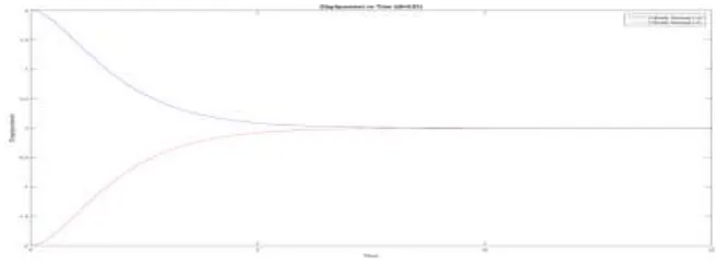
This solution contains two decaying exponentials and oscillating cosine and sine terms. Thus we can predict that the mass will oscillate about the point of rest with an exponentially decreasing amplitude, eventually coming to rest. The following MATLAB graph demonstrates the displacement response of an under damped system (in this case a harmonic oscillator).
Figure1: Graph for displacement vs time for an under damped mass-spring system
Critically Damped
319 | P a g e
critical damping coefficient of the system. In this case, the characteristic equation will produce only one root. The following example illustrates a critically damped harmonic oscillator.The equation used in this instance is –
This factors into –
Thus we have the real
root s = -1. The general solution is therefore –
We know that k1e-t 0 as t ∞. However, in the expression k2te-t , we have a ‘t’ term which goes to infinity
multiplied by a term which goes to zero. We can rewrite the second expression as –
Now we have an expression where both the numerator and denominator go to infinity. At this point we can use l’Hopital’s rule which says that the limit of a function whose numerator and denominator both go to infinity is the same as that of its derivative;
Thus we have –
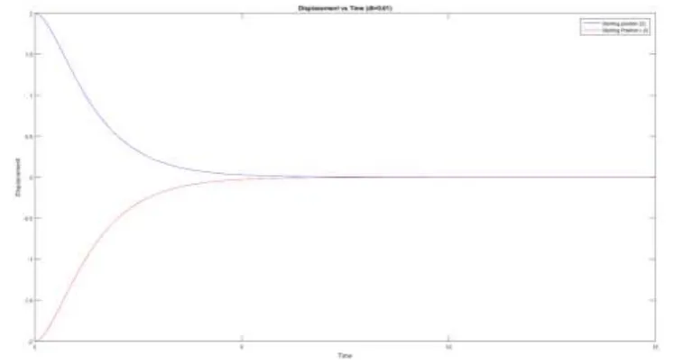
Now we know that the second expression in (25) also goes to zero. Thus we’ll expect the amplitude of the mass
to decrease relatively quickly down to the rest position.The following MATLAB graph demonstrates the
displacement response of a critically damped system.
320 | P a g e
Overdamped:
(b>0 & b >bc)
An overdamped system can be achieved when the spring constant is equal to 2 and the damping constant is 3, for example, forming the following differential equation:
This gives the following differential equation:
This results in the roots s1 = -1 and s2 = -2. Hence the general solution becomes:
The following graph comes from MATLAB. The code used describes an unforced mass-spring system. The code for all MATLAB graphs can be found in the appendix section of this report.
There are no units for the ‘displacement’ and ‘time’ variables in the following graph as the units are arbitrary.
Figure 3 - Graph of Displacement Vs Time for an overdamped 1DOF spring-mass system
Forced Oscillator:
Let the following differential equation be used as an example:
321 | P a g e
Thus the roots are s = -2, -1If we solve for the homogeneous version of this equation we obtain the following solution –
Thus the unforced oscillator will tend to zero. In order to find a solution to the forced oscillator, we need to
guess a possible solution. Asin(t) and Bcos(t) can’t be solutions because the y’ term gives a cosine term in the
case of Asin(t) and vice versa in the case of Bcos(t). Guessing a combination of the two, however, works: Asin(t)
+ Bcos(t).
Plugging in this into equation (27) gives the solution A = 3/10 and B = 1/10. Thus any solution of this equation is of the form –
Since the first two terms will always tend to zero regardless of what k2is, the solution will always end up as –
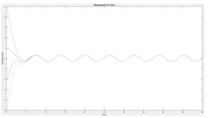
This is the steady-state solution and has a period of 2 , which is the frequency of the forcing term. The following graph from MATLAB illustrates this behaviour. Four separate starting points are taken and the system always ends up oscillating at the same frequency as the input force, regardless of the starting position.
322 | P a g e
The different starting points in the above graph are – 1 unit above zero (blue line), 2 units below zero
(purple line), 5 units below zero (yellow line) and 5 unites above zero (orange line).
Forced Oscillator without damping
Let the following differential equation be used as an example:
The homogeneous equation then becomes:
Thus the general solution to the homogeneous equation is:
The solution to this equation does not reduce to rest, and to obtain the full non-homogeneous solution we make a similar guess as before; Asin(t) and Bcos(t). Putting this into the differential equation we get:
This means that and A = 0. Thus the particular solution to the differential equation:
Now we’ll look at what happens to the system when the forcing term’s frequency is set at different values.
At
323 | P a g e
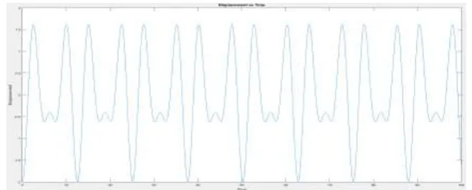
The response seen is visibly periodic, however it doesn’t display a smooth sine response as seen in the earlier response.With the forcing frequency as an irrational number, the above graph shows that the motion of the
mass is no longer periodic.At
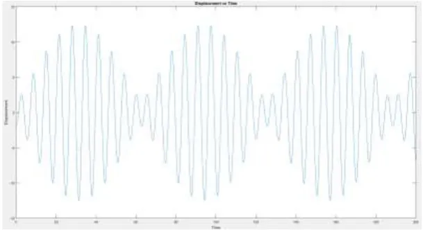
Figure 7 - Displacement vs Time of undamped, forced harmonic oscillator with
The response seen above is a good example of the ‘beats’ phenomenon. ‘Beats’ are produced when the frequency of the external input is extremely close to, but not equal to the natural frequency of the system.
Finally, when :
In this new case, a solution in the form of: Acos(t) + Bsin(t) cannot be used, as this is a solution for a
homogenous equation. As this is a non-homogenous equation. Hence a new solution must be assumed, and is in the form of:
Substituting this into the above differential equation then gives:
Thus:
324 | P a g e
Assuming initial conditions y(0) = 0 and y’(0) = 0 , the solution which satisfies these conditions is:It can clearly be seen that the displacement y(t) is directly proportional to the time t. Hence, the amplitude of the displacement will proportionately increase with time, and can be seen in the figure MATLAB output below.
This phenomenon is known as resonance. Hence, the phenomenon of increase in the amplitude of oscillation
when a system is exposed to a periodic force, whose frequency is equal to the undamped natural frequency of the system is called resonance.
Figure 8 - Displacement vs Time for undamped, forced harmonic oscillator with
Resonance is generally considered to be harmful, and can have devastating effects on engineering structures when triggered. This is discussed in a later section, which talks about the collapse of the Tacoma Narrows Bridge in 1940. It can however be useful in a system. An example where resonance is essential is in wireless electricity transfer using inductive coupling. The primary and secondary coils must have a certain number of turns, with the right frequency of current in order for them to resonate with each other.
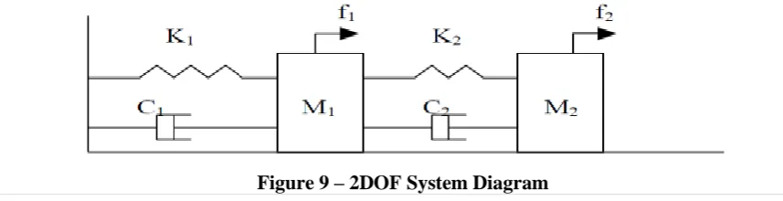
II MATLAB IMPLEMENTATION OF 2DOF SYSTEM
In order to use MATLAB to compute the response to a 2DOF system, a slightly simpler variant of the
system described earlier will be used. Instead of the system having three springs and three dampeners,
a system having two masses, two springs and two dampeners will be used instead. The system
diagram is given below:
325 | P a g e
The specific matrices used to produce the graph below are as follows:Figure 10 - Amplitudes of two masses vs Frequency ratio
The above graph represents the displacement response of the 2DOF system with the variance of the frequency
ratio nusing the input parameters given earlier. The two observable peaks seen on the graph represent the
326 | P a g e
could be tuned such that the anti-resonating frequency is hit constantly instead. This would drastically reduce the vibrations caused due to resonance.III CONCLUSION AND FUTURE OUTLOOK
This report was focused on the spring mass system, with a comparative usage of MATLAB and numerical methods like Euler’s method, the Euler Cromer method and the Runge-Kutta method to find and solve the equations of motion of the various systems discussed. The report initially analysed a Single DOF system, describing the effects and implications of both forced and unforced systems. It then went on to discuss the various types of damping, namely the underdamped, critically damped and overdamped conditions.
A forcing term was then introduced to the system, and the system’s response was plotted into several graphs using MATLAB. These graphs illustrated the effects of the forced input at different frequency ratios. Instances
where the frequency ratio, nwas equal to 1.5, , 0.9 and 1.0. Each case produced an interesting non
trivial output. When the frequency ratio was an interesting response of jagged waves were seen in stark
contrast to the smooth sine waves normally observed. Another interesting response was noted when the frequency ratio was equal to one, with the phenomenon of resonance being observed. The system responses of the damped 1DOF system from an analytical perspective and through MATLAB were then compared, and it was seen that the steady state response was always in phase with the forced input.
A simple 2DOF system with two masses, three springs and three dampeners then introduced, and the underlying mathematical derivation of the steady state response was deliberated upon. A MATLAB implementation of an undamped 2DOF system was undertaken, with a focus on the description of the displacement of masses vs frequency and phase of masses vs frequency responses. It was seen that when the frequency ratio was raised in steps of 0.1, the displacements would always drop down to zero (or extremely close to it) before steeply rising again. It was also seen that the phases would vary by 180 degrees each time the frequency ratios were increased by 0.1.
Through this report, a firm belief that an understanding of wave dynamics and vibration control is critical in the proper functioning of engineering structures. Resonance can prove disastrous, but can also be harnessed and used in applications like wireless electricity transfer and radio wave enhancements.
References
[1]Wikipedia, 4/02/2015, “Symplectic Integrator”, viewed 10/04/2015, http://en.wikipedia.org/wiki/Symplectic_integrator
[2]Astrophysics at North Carolina State University, “Introduction to Scientific Computing”, North Carolina State University, viewed 10/04/2015,
http://astro.physics.ncsu.edu/~cekolb/urca/lessons/14.html
[3]Introduction to Dynamics and Vibrations, “5.5 Introduction to vibration of systems with many degrees of freedom”, School of Engineering - Brown University, viewed 13/04/2015,
327 | P a g e
[4]Howard. P, 2009, “Solving ODE in MATLAB”, viewed 10/04/2015[5]Introduction to Aerospace Structures (ASEN 3112), “MDOF Dynamic Systems”, Department of Aerospace Engineering Sciences – University of Colorado at Boulder, 2014, Lecture 19, p.1-24, viewed 15/05/2015 [6]Wikipedia, 27/05/2015, “Runge-Kutta Methods”, viewed 28/05/2015,
http://en.wikipedia.org/wiki/Runge%E2%80%93Kutta_methods