Earthquake Source Characterization Through Seismic Observations and Numerical Modeling

(1)

seismic observations and numerical modeling

Thesis by

Semechah K. Y. Lui

In Partial Fulfillment of the Requirements for the degree of

Doctor of Philosophy

CALIFORNIA INSTITUTE OF TECHNOLOGY Pasadena, California

2017

(2)

(3)

ACKNOWLEDGEMENTS

The acknowledgments is perhaps the hardest part of this thesis, as I find it difficult to put my gratitude into words. This work would not have been possible without a lot of people.

First and foremost, my sincere gratitude goes to my research advisers, Don Helm-berger and Nadia Lapusta. Don gave me a warm welcome to the world of seismology. Even until this day, I am inspired by his sharpness in generating countless research ideas and asking interesting questions. Sometimes I went into his office with several questions, and came out with even more. Nonetheless, I have learned a lot from our meetings. Don also showed tremendous support and encouragement through the ups and downs of doing research. I will truly miss our discussion time, his wittiness, and his warm smile. Nadia motivates me to strive to be a diligent researcher. She is an excellent teacher, who understands my confusion even before I can articulate it clearly, and her clarity in explaining complicated physics is something I admire. I thank her for her willingness to spend long hours discussing my research amid her busy schedule. I am always grateful for her help and advice.

I owe my special thanks to my undergraduate research adviser, Eric Hetland, who took me step by step into the world of research. I am grateful for his patience and trust in me when I started as a clueless research assistant in my sophomore year. I would not have made it to graduate school without his encouragement and guidance all along.

I also thank other members in my thesis advising committee, Jean-Paul Ampuero, Jean-Philippe Avouac, Rob Clayton, and Victor Tsai, for the time they dedicated to my thesis and its progress. Many others have been my research mentors and collaborators on various projects. I thank Zhongwen Zhan, Shengji Wei, Robert W. Graves, Xiangyan Tian, Junle Jiang, Ting Chen, and Yihe Huang for their insightful advice and discussions.

(4)

Ting Chen, Jeff Thompson, Franklin Koch, Yiran Ma, Voonhui Lai, Jorge Castillo Castellanos and Zhichao Shen - for all the intellectual discussions, fun chats, and yummy snacks that we share, which make SM362 a friendly and productive place to work in. I would also like to extend my gratitude to the administrative staff, Donna, Priscilla, Kim, Rosemary, and Sarah, who are always caring and helpful.

Outside of school, the Chinese Bible Missions Church is my second home in Los Angeles. I thank a lot of brothers and sisters for being great role models and for adding so much color to my life here in Los Angeles. Many of them have welcomed and treated me as part of their families. I will miss our time in worship practices, fellowship programs, Bible study sessions, discipleship training, Sunday school lessons, and simply hanging out. I am grateful that God has brought us together in this journey of Faith.

I would also like to thank VaiMan & Vennis Lei, and Amy & Joseph Ho, for taking good care of me throughout my graduate studies here. Nick & Cheri Lam, and Joey Fung are wonderful friends and mentors during difficult times. I am thankful for the precious friendships that we share.

My heartfelt gratitude goes to my family - Dad, Mom, and my sister Ji - who are my anchors to help me stay grounded. I thank them for their support in my decision to study abroad and for sending their unfailing love across the Pacific over the past nine years. Ji is the best sister one could ask for and my role model in life.

(5)

ABSTRACT

In this thesis, I present a series of works on the characterization of source properties and physical mechanisms of various small to moderate earthquakes through both observational and numerical approaches. From the results, we find implications on a broader scheme of topics relating to larger earthquakes, shear zone structure, frictional properties of faults, and seismic hazard assessment.

Part I consists of two studies using waveform modeling. In Chapter 2, we present an in-depth study of a series of intraslab earthquakes that occurred in a localized region near the downdip edge of the 2011Mw Tohoku-Oki megathrust earthquake.

By refining source parameters of selected events, simulating their rupture properties and comparing their mechanisms to stress changes caused by the main shock in the region, we are able to identify the true rupture plane and the reactivation of a subducted normal fault, enhancing our understanding on the downdip shear zone. In Chapter 3, based on similar techniques, we further develop a systematic methodology to perform fast assessments on important source properties as an earthquake occurs. For two Mw 4.4 earthquakes in Fontana, moment magnitude and focal mechanism

can be accurately estimated with 3 to 6 s after the first P-wave arrival, while focal depth can be constrained upon the arrival of S waves. Rupture directivity can also be determined with as little as 3 seconds of P waves. This study opens the opportunity to predict ground motions ahead of time and can potentially be useful for Earthquake Early Warning.

(6)

(7)

PUBLISHED CONTENT AND CONTRIBUTIONS

Lui, Semechah KY, Don Helmberger, Shengji Wei, Yihe Huang, and Robert W Graves (2015). “Interrogation of the Megathrust Zone in the Tohoku-Oki Seismic Region by Waveform Complexity: Intraslab Earthquake Rupture and Reactivation of Subducted Normal Faults”. In:Pure and Applied Geophysics172.12, pp. 3425– 3437. doi: 10.1007/s00024-015-1042-9. url:http://dx.doi.org/10.

1007/s00024-015-1042-9_.

Lui and Helmberger co-designed the study. Lui generated all the 1D synthetic seismograms, analyzed both the 1D and 3D velocity models, performed seismic waveform inversions and the analysis on earthquake rupture properties, and wrote the manuscript. Graves and Wei generated all the 3D synthetic seismograms. Huang contributed to calculating the regional stress change. All authors con-tributed to interpreting the results. Lui and Helmberger finalized the manuscript. Lui, Semechah KY, Don Helmberger, Junjie Yu, and Shengji Wei (2016). “Rapid Assessment of Earthquake Source Characteristics”. In: Bulletin of the

Seismo-logical Society of America 106.6, in press. doi: 10 . 1785 / 0120160112. url:

http://dx.doi.org/10.1785/0120160112_.

Lui and Helmberger co-designed the study. Lui performed all the seismic wave-form inversions and directivity analysis for the targeted earthquakes in Fontana, and wrote the draft of the manuscript. Yu and Wei contributed to the prelim-inary studies on the earthquakes in Chino Hills and in Brawley. Both Lui and Helmberger contributed to interpreting the results and finalizing the manuscript. Lui, Semechah KY and Nadia Lapusta (2016). “Repeating microearthquake se-quences interact predominantly through postseismic slip”. In:Nature

Communi-cations7, p. 13020. doi:10.1038/ncomms13020. url:http://dx.doi.org/

10.1038/ncomms13020_.

(8)

LIST OF ILLUSTRATIONS

Number Page

2.1 Overview of the study region. . . 9

2.2 Earthquakes at the downdip edge of the Tohoku-Oki rupture region. . 10

2.3 Comparison between 1D and 3D synthetic waveforms of event E1. . . 13

2.4 Timing shift and cross-correlation between data and 1D synthetics waveform. . . 14

2.5 Synthetic waveform comparison of event E1 generated from two different 3D velocity models. . . 15

2.6 Comparison of focal mechanisms from CAP inversion. . . 16

2.7 Rupture directivity as shown from waveform data. . . 17

2.8 Modeling rupture directivity using the empirical Green’s function approach. . . 18

2.9 Stress change in the ruptured region due to the Mw 9.1 mainshock. . . 20

2.10 Comparison of the difference in time shift values of E1 and E2 assuming different epicentral locations. . . 22

2.B1 Waveform inversion with frequency bands up to 0.05 Hz. . . 25

2.B4 Waveform inversion with frequency bands up to 1 Hz. . . 28

2.B5 Detailed analysis result of CAP inversion. . . 29

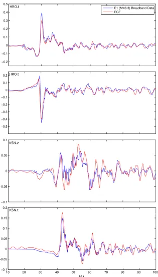
2.B6 Comparison of E1 broadband displacement data and EGFs at two of the nearest stations HRO and KSN. (vertical and tangential compo-nents respectively) . . . 30

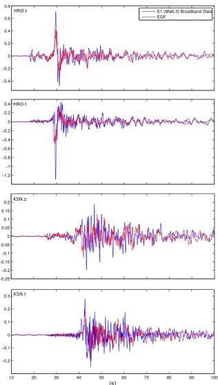
2.B7 Comparison of E1 broadband velocity data and EGFs at two of the nearest stations HRO and KSN (tangential and vertical components respectively). . . 31

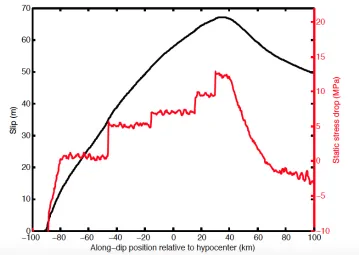
2.B8 Final slip and static stress drop of the main event. . . 32

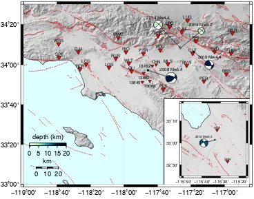
3.1 Overview of the study region of this project near the city of Fontana located near the San Andreas Fault. . . 40

3.2 Preliminary test on the 2012 Brawley event. . . 41

(11)

3.4 Stations near the epicenters are selected for rapid assessment of source

parameters. . . 45

3.5 CAP allows accurate and fast characterization of moment magnitude, focal mechanism and depth. . . 46

3.6 Directivity observed from difference in amplitude ratio of waveform across all azimuths. . . 47

3.7 Predicting rupture directivity using incoming P-wave. . . 48

3.8 Sensitivity test of waveform at different frequency bands. . . 49

3.9 We can predict the amplitude of S-wave arrivals based on the P-wave directivity analysis. . . 50

3.10 Simulating Green’s functions of larger earthquakes using the EGF approach. . . 52

3.A1 Preliminary study on the 2008 Chino Hills earthquake. . . 54

3.A2 Waveform recorded at stations within the LA Basin. . . 55

3.A3 The study on the Inglewood Mw 4.6 earthquake by Luo et al (2010). . 56

3.A4 Waveform inversion of the two events using the whole network. . . . 57

3.A5 Small event can be used as EGFs for studying directivity. . . 58

3.A6 Detailed results of the directivity analysis with 3 s of incoming P wave. 59 3.A7 Validating the ground-motion prediction test with the EGF approach. 60 3.A8 Rayleigh wave prediction for the same four stations. . . 61

4.1 Interaction of two repeating earthquake sequences in a rate-and-state fault model. . . 74

4.2 Exploring the extent of interaction. . . 75

4.3 Different types of stress changes induced on the triggered VW patch. 76 4.4 Effect of the VS region on the interaction. . . 77

4.B1 Cumulative slip along the fault through time. . . 80

4.B2 Selecting initial conditions for simulations that allow us to quantify the potential interaction between the repeating sequences. . . 81

4.B3 Example of initial conditions on the fault. . . 82

4.B4 Comparison of the single-patch and two-patch simulations . . . 83

4.B5 Interaction of two VW patches - Case 1. . . 84

4.B6 Interaction of two VW patches - Case 2. . . 85

4.B7 Behavior of postseismic creep on faults with different velocity-strengthening friction properties(a−b)VS. . . 86

(12)

4.B9 Similar to Figure 4.B8, with a different definition of ζ . . . 87 4.B10 Interaction of two VW patches - Case 3. . . 88

5.1 Repeating earthquake sequences on the portion of the Parkfield seg-ment of the San Andreas Fault. . . 97 5.2 Fault properties in M1 and M2. . . 104 5.3 Simulation results for (a) M1-b, (b) M2-b, and (c) M2-d with(a−b)VS

= 0.008. . . 106 5.4 comparison of the ratio of seismic to aseismic slip in different

recur-rence periods in M1-b. . . 109 5.5 Effect of interseismic events on the repeating sequence in M2-b. . . . 110 5.6 comparison of the ratio of seismic to aseismic slip in different

recur-rence periods in M2-b. . . 112 5.7 Comparison of the average shear stress on the VW patch in M1 and M2113 5.8 Tr vsMofor the repeating events in M1, M2, and M3. . . 114

5.9 Example of model set up for simulating the SF and LA repeating sequences. . . 116 5.10 Example of the interaction between the SF and LA events, from

M1-double with(a−b)VS= 0.004. . . 117

5.11 Interactions between the SF and LA patch in models M1-double and M2-double, with(a−b)VS = 0.004. . . 119

5.12 Comparison of the interaction among VW regions between single-patch and double-single-patch cases. . . 120 5.13 Source properties of the repeaters in models with a larger extent of

spatial heterogeneity. . . 121 5.14 Another example illustrating the effect of spatial heterogeneity on

faults. . . 122 5.15 Dependence of the postseismic creep on the frictional properties of

the VS region. . . 123 5.16 Suppression of the postseismic creep on a strongly velocity-strengthening

segment with(a−b)VS= 0.032. . . 124

5.17 Frictional properties of the creeping segment significantly affect the source properties of the repeaters. . . 125 5.18 Frictional properties of the creeping region affect the average stress

(13)

LIST OF TABLES

Number Page

2.B1 1D crustal model for the Tohoku-Oki region studied. . . 32

2.B2 Result of directivity simulations based on displacement data . . . 33

2.B3 Result of directivity simulations based on velocity data . . . 33

3.A1 1D crustal model for the Southern California region studied . . . 61

4.A1 Parameters of Our Simulations . . . 79

4.B1 Summary of the eventual event pattern for a range of VW patch sizes d and initial conditions. . . 89

5.1 Fault model parameters used for all simulations . . . 101

5.2 Hydrothermal properties of the VW patch in M1 . . . 104

5.3 Fault parameters used in M1 and M2 and properties of the reproduced seismic sources. . . 106

5.4 Comparison between the repeating sequences reproduced in M2-e and M3. . . 108

(14)

NOMENCLATURE

Directivity. Direction of rupture on a fault during an earthquake.

Fault strength. The ability of a fault to withstand an applied shear stress.

Focal mechanism. Fault-plane solution describing the deformation in the source

region that generates the resulting seismic waves.

Moderate earthquake. 5≤ Mw ≤ 7.

Pnl waves. The entire wavetrain between P and S waves.

Rise time. Local duration of slip during an earthquake.

Slip. The relative displacement at a given position on the fault.

Small earthquake. M_w ≤_5.

Stress drop. The difference in shear stress on a ruptured fault before and after an

(15)

C h a p t e r 1

INTRODUCTION

The earliest earthquakes with descriptive information can be traced back to over 3000 years ago. Throughout history, the Earth has demonstrated its dynamic nature. Numerous records of damages caused by the intense shaking can be found in the literature, with events spanning a wide range of magnitudes (Mw) and occurring in

different tectonic settings and at unpredictable times. In the ancient days, people relied on creative stories to explain the sudden movements of the Earth’s crust, including a giant twitchy catfish named Namazu in Japan, and the angry Poseidon, the god of the sea in Greece. The true natural cause of earthquakes has long been a mystery until the 18t h century.

In modern days, technological advancement has allowed seismologists high-resolution seismic wave observation by broadband seismometers, increasing our scientific un-derstanding of earthquake processes. Nonetheless, due to the complexity of seismic sources, as well as their intricate interplay with the Earth’s heterogeneous struc-ture, scientists are continuously surprised by what happens in nature. For example, the largest seismic slip of the Tohoku-Oki Mw 9.1 megathrust earthquake actually

occurred close to the trench where stable creeping was expected (Ide et al., 2011; Loveless and Meade, 2010; Simons et al., 2011; Wei et al., 2012). Also, the reason behind the absence of great historic earthquakes on the southern San Andreas Fault in California remains uncertain (Fialko, 2006). These examples point to the fact that earthquake physics is still a tough nut to crack.

(16)

can we characterize about an earthquake as it happens, and how fast can we do it? Can smaller earthquakes help us constrain the maximum size of earthquakes that can potentially happen in a seismogenic zone? Can one predict the source behavior of future large earthquakes by studying small events in the region? Can small earthquakes tell us the controlling factors for slip and rupture on a fault? The focus of this thesis is on various observations of small to moderate earthquakes in subduction zones and on transform faults, with moment magnitude (Mw) between

1.5 and 6.5. Due to generally insufficient seismic data resolution and azimuthal coverage, it has been challenging to characterize smaller earthquake sources, and so they are usually regarded as simple radially symmetric rupture at a constant rupture velocity (Brune, 1970; Eshelby, 1957; Madariaga, 1976). In contrast, the ruptures of larger earthquakes ruptures are found to be more complex, often propagate in a unilateral fashion (Henry and Das, 2001; Mai et al., 2005; McGuire et al., 2002). In the past, however, a limited number of studies have shown that small events do have more complicated source processes than typically assumed (Boatwright, 2007; Domański et al., 2002). Fortunately, the rapid densification of regional and global seismic networks and the advancement of computational resources in recent years enable integrated approaches to study the physics of earthquakes, as well as making detailed analysis of small earthquakes possible. On one hand, high-resolution waveform modeling allows in-depth understanding of the kinematics of source processes. On the other, recently developed dynamic rupture simulations consider the effect of seismic wave interactions and are capable of producing realistic rupture behavior that can be compared to observations, providing insights into the fundamental physics that drives what we see on real faults. Furthermore, numerical modeling also bridges the gap between tiny laboratory earthquakes and megaearthquakes (Mw >9) in nature.

In the following chapters, we present a series of studies that exemplify the utilization of (I) observational and (II) numerical approaches to characterize small to moderate earthquake sources in various tectonic settings and their driving physics. We aim to determine from the wealth of data what smaller earthquakes can tell us about tectonics and larger earthquakes.

1.1 Earthquake characterizations through seismic observations

(17)

seismic waves in order to accurately and efficiently constrain the source and rupture properties.

Chapter 2 illustrates how source properties can be useful in delineating local crustal structures and verifying the state of stress in the region. Here we focus on a group of moderate earthquakes (Mw 4.5 to 6.5) that occurred after the 2011Mw 9.1

Tohoku-Oki megathrust event on the downdip edge of the ruptured area. Using broadband waveform modeling, we refine their source parameters, including their focal mech-anisms, focal depths, and rupture properties, such as direction and dimension. We discover that these events align in a narrow strip inside the subducting slab, which is potentially the result of the reactivation of a subducted normal fault. Through resolving the rupture properties of these intraslab earthquakes, the orientation of this fault can be determined. Furthermore, focal mechanisms of these events are also shown to have a causal relationship with the stress change caused by the mainshock. This study highlights the importance of precise source properties in uncovering the features and evolution of the background tectonic region.

In Chapter 3, we investigate the potential of rapid and accurate source characteri-zation and its implications in the field of Earthquake Early Warning (EEW). The tectonic setting here changes from a subduction zone to a mature transform fault system. With several small events (Mw 3-4.5) in Fontana, California, we introduce

a methodology in which source and rupture properties can be constrained within as little as 3 seconds of the arriving seismic waves, which provides valuable infor-mation for the prediction of the associated ground motion in broader regions from the epicenter. We also demonstrate how one can effectively calculate the potential ground motion of a larger event using past events in the same location via empirical Green’s functions. This study highlights the importance of establishing efficient source characterization for hazard assessment and response.

1.2 Numerical simulations of earthquake physics

Motivated by intriguing observations, in Part II, we use dynamic fault simulations to study seismic sources and their supporting physics, with a particular focus on earthquakes that interact with one another. To this end, we explore the cause of earthquake triggering, based on a dynamic rupture model governed by rate-and-state friction laws.

(18)

that occur between the repeating events. One major finding is that postseismic creep dominates the interaction in the models. Because of this, earthquake triggering in our model also occurs at distances much larger than typically assumed. Since the behavior of postseismic creep depends heavily on the frictional properties of the fault on which it propagates, these findings further emphasize the importance of source characterization in constraining properties of creeping segments.

Lastly, in Chapter 5, we integrate results from Chapter 4 with field observations by applying the fault model to reproducing the interacting microearthquakes found on the Parkfield creeping segment of the San Andreas Fault. Apart from the unique interacting seismic pattern in previous studies, these repeaters are also characterized by anomalous source properties, such as high stress drops on the order of 30 to 60 MPa. We show that dynamic rupture simulations are able to provide an explana-tion for the phenomena. The high stress drops can be reproduced in a rate-and-state fault model when additional factors are present on the velocity-Weakening patches; two possibilities are thermal pressurization of pore fluids and locally elevated nor-mal stress. Our results show that the variability of the source properties and the interactions of these repeaters, as well as their observed scaling between recurrence timeTr and seismic moment Mo, are due to the occurrence of substantial aseismic

slip on the velocity-weakening patches. We also discuss the effect of frictional properties of the creeping region on both the behavior of postseismic slip and the source properties of these repeaters.

Chapters 2 to 4 of this thesis are published in peer-reviewed journals, while Chapter 5 will be submitted for publication with additional modeling results.

1.3 References

Boatwright, John (2007). “The persistence of directivity in small earthquakes”. In: Bulletin of the Seismological Society of America97.6, pp. 1850–1861. doi:

10.1785/0120050228_{. url:}http://dx.doi.org/10.1785/0120050228_.

Brune, James N. (1970). “Tectonic stress and the spectra of seismic shear waves from earthquakes”. In:Journal of Geophysical Research75.26, pp. 4997–5009. issn: 2156-2202. doi: 10.1029/JB075i026p04997. url: http://dx.doi.

org/10.1029/JB075i026p04997_.

Domański, B, SJ Gibowicz, and P Wiejacz (2002). “Source time function of seismic events at Rudna copper mine, Poland”. In:The Mechanism of Induced Seismicity. Springer, pp. 131–144. doi: 10.1007/PL00001247. url: http://dx.doi.

(19)

Eshelby, John D (1957). “The determination of the elastic field of an ellipsoidal inclusion, and related problems”. In:Proceedings of the Royal Society of London

A: Mathematical, Physical and Engineering Sciences. Vol. 241. 1226. The Royal Society, pp. 376–396. doi:10.1098/rspa.1957.0133. url:http://dx.doi.

org/10.1098/rspa.1957.0133_.

Fialko, Yuri (2006). “Interseismic strain accumulation and the earthquake potential on the southern San Andreas fault system”. In:Nature441.7096, pp. 968–971. doi:

10.1038/nature04797_{. url:}http://dx.doi.org/10.1038/nature04797_.

Henry, C and S Das (2001). “Aftershock zones of large shallow earthquakes: fault dimensions, aftershock area expansion and scaling relations”. In: Geophysical

Journal International147.2, pp. 272–293. doi:10.1046/j.1365-246X.2001.

00522.x_{. url:}http://dx.doi.org/10.1046/j.1365-246X.2001.00522.

x_.

Ide, Satoshi, Annemarie Baltay, and Gregory C Beroza (2011). “Shallow dy-namic overshoot and energetic deep rupture in the 2011 Mw 9.0 Tohoku-Oki earthquake”. In: Science 332.6036, pp. 1426–1429. doi: 10.1126/science.

1207020_{. url:}http://dx.doi.org/10.1126/science.1207020_.

Loveless, John P. and Brendan J. Meade (2010). “Geodetic imaging of plate motions, slip rates, and partitioning of deformation in Japan”. In:Journal of Geophysical

Research: Solid Earth115.B2. B02410, n/a–n/a. issn: 2156-2202. doi:10.1029/

2008JB006248_{. url:}http://dx.doi.org/10.1029/2008JB006248_.

Madariaga, Raul (1976). “Dynamics of an expanding circular fault”. In:Bulletin of

the Seismological Society of America66.3, pp. 639–666.

Mai, P Martin, P Spudich, and J Boatwright (2005). “Hypocenter locations in finite-source rupture models”. In:Bulletin of the Seismological Society of America95.3, pp. 965–980. doi: 10.1785/0120040111. url: http://dx.doi.org/10.

1785/0120040111_.

McGuire, Jeffrey J, Li Zhao, and Thomas H Jordan (2002). “Predominance of uni-lateral rupture for a global catalog of large earthquakes”. In:Bulletin of the

Seis-mological Society of America92.8, pp. 3309–3317. doi:10.1785/0120010293.

url:http://dx.doi.org/10.1785/0120010293.

Simons, Mark et al. (2011). “The 2011 magnitude 9.0 Tohoku-Oki earthquake: Mosaicking the megathrust from seconds to centuries”. In: science 332.6036, pp. 1421–1425. doi: 10 . 1126 / science . 1206731. url: http : / / dx . doi .

org/10.1126/science.1206731_.

Wei, Shengji, Robert Graves, Don Helmberger, Jean-Philippe Avouac, and Junle Jiang (2012). “Sources of shaking and flooding during the Tohoku-Oki earth-quake: A mixture of rupture styles”. In:Earth and Planetary Science Letters333, pp. 91–100. doi: 10.1016/j.epsl.2012.04.006. url: http://dx.doi.

(20)

C h a p t e r 2

INTERROGATION OF THE MEGATHRUST ZONE IN THE

TOHOKU-OKI SEISMIC REGION BY WAVEFORM

COMPLEXITY: INTRASLAB EARTHQUAKE RUPTURE AND

REACTIVATION OF SUBDUCTED NORMAL FAULTS

Lui, Semechah KY, Don Helmberger, Shengji Wei, Yihe Huang, and Robert W Graves (2015). “Interrogation of the Megathrust Zone in the Tohoku-Oki Seismic Region by Waveform Complexity: Intraslab Earthquake Rupture and Reactivation of Subducted Normal Faults”. In:Pure and Applied Geophysics172.12, pp. 3425– 3437. doi: 10.1007/s00024-015-1042-9. url:http://dx.doi.org/10.

(21)

ABSTRACT

Results from the 2011Mw9.1 Tohoku-Oki megathrust earthquake display a complex

(22)

2.1 Introduction

2.1.1 Background: Complexity of the Tohoku-Oki Seismic Region

The Mw 9.1 Tohoku-Oki earthquake in 2011 devastated the Northeast coastline

of Japan. Analysis of various data sets (i.e. regional and teleseismic broadband seismographic networks, geodetic networks, ocean-bottom measurements, etc.) demonstrates a unique and complex rupture pattern which indicates varying me-chanical and frictional properties along the thrust zone (Fujiwara et al., 2011; Ide et al., 2011; Ito et al., 2011; Simons et al., 2011; Wei et al., 2012; Yue and Lay, 2011). Especially intriguing is the difference of frequency content in radiated en-ergy emanating from various parts of the rupture zone. Huang et al., (2012) show that the high-frequency radiations in the deeper part are at least partially caused by asperities that have hosted earthquakes before, but the exact mechanism that has caused the variation of such energy concentration is currently unclear. Since the mainshock, the region has also experienced a sharp increase in seismic aftershock activity. These seismic events span a wide range in size and depth. Current national and international earthquake catalogs rely mainly on travel-time data to determine origin time and spatial location. Unfortunately, their results often do not agree, where the hypocentral locations of earthquakes reported by different networks can vary by over 20 km laterally, and by over 10 km vertically depending on the catalog (Zhan et al., 2012). Furthermore, due to the lack of regional stations on the Pacific side, the resolution decreases with distance from the Japan coast. Such discrepancy creates difficulty in constructing a coherent picture of the thrust zone.

(23)

141˚ 142˚ 143˚ 144˚ 37˚

38˚ 39˚

0 500 1000 1500 2000 2500 3000 3500 4000 4500 5000

Slip (cm)

10

20

30 40 50 60

HRO KSK

KSN

39°

38°

37°

141° 142° 143° 144°

Mw 7.1

Mw 6.3

Figure 2.1: Overview of the study region. (Top left) Map of the Tohoku-Oki region. Dashed rectangular box is the area of the map shown on the right. (Right) Seismic events in the region 141.5 to 142E and 37 to 39N. Focal mechanisms marked in red represent theMw7.1 aftershock and E1 (2011/08/19,Mw6.3) analyzed in this study.

FM marked in green are other seismic events with similar strike, dip and hypocenter depth to the two larger events. FM in yellow are similar events found outside of the rectangular region. Triangles in cyan are the three closest F-net stations to E1. The color scale represents the slip distribution of the Mw 9.1 main shock in 2011

(Wei et. al., 2012). Dotted lines are the slab contours. (Bottom left) Schematic diagram illustrating the formation of normal fault in the outer rise region which later undergoes subduction and reactivation after the Mw 9.1 Tohoku-Oki event.

this group of intraslab earthquakes, the largest is a Mw 7.1 aftershock that occurred

on April 7, 2011, a month after the Mw 9.1 earthquake. Based on detailed seismic

(24)

Figure 2.2: Earthquakes at the downdip edge of the Tohoku-Oki rupture region. These seismic events have displayed very similar focal mechanism and waveform complexity. Waveform (in velocity) shown here are examples recorded by the F-net station HRO: (blue) vertical component showing the behavior of P and SV phases,(red) tangential component showing the behavior of SH phase. Note the similarity in recording from events labeled E2 and E1.

These intriguing observations, as well as the lack of a comprehensive understanding of these intraslab events, have prompted us to investigate this group of earthquakes. In particular, we explore the scope of details that we can extract from existing data, and, by modeling these intraslab events, we test the hypothesis of weakened zones present inside the slab. We also study their correlation with shear stress change in the region caused by the mainshock.

2.1.2 Overview of Our Study

(25)

rupture plane. This section focuses on two intraslab earthquakes within the group, one of which, occurred on August 19, 2011 with Mw 6.3 (named E1, Figure 2.2),

while the other occurred seven months later on March 25, 2012 withMw5.2 (named

E2). According to the JMA catalog, these two earthquakes have almost identical hypocenters, with a lateral separation of less than 4 km and a 1.8-km difference in depth. Their seismic waveform data also have very similar shapes and frequency content as displayed in Figure 2.2. Thus, there is strong evidence indicating that the two earthquakes have occurred at almost the same hypocenter location with similar focal mechanism, but with a difference in moment magnitude. Looking closely at both sets of data, we discover suggestive features of E1 rupturing unilaterally. To verify our hypothesis, E2 is used as the empirical Green?s functions to simulate E1 (Hartzell, 1978). Using Taylor-series expansion in time domain, E1 is modeled as the summation of a line of point sources (Song and Helmberger, 1996). This search procedure allows the determination of the focal plane on which the earthquake occurred, and gives a robust estimation of fault finiteness. These results, together with the other intraslab events in the region with similar mechanisms, suggests a line of weakness at least 150 km long, which is consistent with the estimation in an earlier study by Kato and Igarashi, (2012).

As an extension from our modeling result, in the last part of the paper, we address the effect of shear stress change caused by the mainshock. While previous studies focus mostly on the shear stress change in the regional scale (Kato et al., 2011; Toda et al., 2011), we study locally the area beneath the downdip edge of the main shock rupture region in order to verify the causal relationship between these intraslab events and the megathrust. Without assuming specific fault geometries or friction coefficients, we evaluate faulting mechanisms that are possible in this location.

2.2 Methods and Results

2.2.1 Validity of 1D Seismic Velocity Models

(26)

intraslab events in a localized megathrust zone, we begin with testing the validity of 1D velocity model (Table 2.B1) by comparing data with 1D and 3D waveform synthetics respectively. In this particular study region, we focus on regional data collected from seismic networks in Japan (F-net, K-net and Kik-net), with most stations within 500 km from the earthquake sources. Here the 3D Japan Integrated Velocity Structure Model (JIVSM; Koketsu et al., 2008) is used, which includes a slab structure. We apply the staggered-grid finite difference technique to model 3D wave propagation (Graves, 1996), with a grid spacing of 0.4 km and synthetic waveform frequency up to of 0.25 Hz. Focal mechanism inversions in this part of the study is done with the 1D Cut-and-Paste (CAP) method, which has the advantage of performing inversion on selected portions of Pnl and surface waves with timing shifts allowed among segments (Zhao and Helmberger, 1994; Zhu and Helmberger, 1996). We performed a detailed comparison between the synthetic waveforms generated with a 1D velocity model and those with 3D velocity models in order to consolidate station paths that are 1D-like.

(27)

13

70 80 90 100 110 120 130 140 150 160 170 180 190 200

Distance, km

-15 -10 -5 0 5 10 15 20 25 30 35 40 45 50

Time(s)

FKS013 TCG005

TCGH10

FKS015 TCG001 TCGH09

FKSH12 TCG002

FKS016

FKS009

FKS031 FKSH11 FKSH10 FKS027

FKS017 FKSH08

FKSH09 FKSH05 FKS025

FKS018

FKS008

FKSH19 FKS024

FKS006 FKSH18 FKSH04

FKS023

FKS020

FKS019 FKS022

FKSH03

FKS005

data_20110819,AZ:240~270,UD,Vel,bp c 0.03 0.25 p 2 n 6140˚E 142˚E 144˚E 36˚N

SUPPL. FIGURE (1)

Comparison between 1D (red) and 3D (black) Synthetics

Figure 2.3: Comparison between 1D (marked in red) and 3D (marked in black)

synthetic waveforms of event E1. Vertical velocity waveform is shown here. Stations selected are between the azimuthal range of 240◦and 270◦, at the nearest distances. A bandpass filter with cutoff frequencies 0.03 and 0.25 Hz is applied to the synthetics. Also, waveforms in the plot are normalized and the 3D synthetics are systematically shifted to arrive earlier by 2 seconds.

(28)

14 Depth (km) to Vs=2.5 km/s NIED

137˚ 138˚ 139˚ 140˚ 141˚ 142˚ 143˚ 144˚ 145˚ 146˚ 33˚

SUPPL. FIGURE (2)

3D Vs Data

1D Vs Data

3D Vs Data 1D Vs Data

Figure 2.4: Timing shift and cross-correlation between seismic data and 1D

syn-thetics waveform. (Left) Stations (triangles) are colored by the cross-correlation coefficients (cc) between 3D synthetics and waveform data (vertical component) of event E1. Only stations with > 70% cc values are plotted. Colored lines indicate time-shift value to align the data and synthetics, ranging from -4 to 4 seconds, with positive value representing faster synthetics. (Right) Similar to figure on the left, ex-cept that this is showing the cross-correlation between 1D synthetics and waveform data.

Lastly, a direct comparison is made between the 1D and 3D synthetics by running 1D CAP inversions with 3D synthetics as data. A substantial number of stations have cc > 70% for significant phases (P and S). Given such results, we are confident in using the 1D CAP results in our following analysis.

2.2.2 Source Mechanism and Rupture Characteristics of Selected Intraslab

Events

(29)

15

80 90 100

Distance, km

-15 -10 -5 0 5 10 15 20 25 30 35 40 45 50 Time(s)

FKS004

FKS0015 MYGH10 MYG017

data_20110819,AZ:270~300,UD,JIVSM vs NIED,bp c 0.03 0.25 p 2 n 6140˚E 142˚E 144˚E

36˚N 38˚N

140˚E 142˚E 144˚E

36˚N 38˚N 40˚N

Ep

ice

nt

ra

l d

ist

an

ce

(km)

SUPPL. FIGURE (3)

Comparison of 3D Synthetics Event ID 20110309 20110310 20110724 20110819 20120325

140˚ 142˚ 144˚

36˚

38˚

40˚ 40°

38°

36°

140° 142° 144°

Figure 2.5: Synthetic waveform comparison of event E1 generated from two different

3D velocity models. (Left) Synthetic waveform comparison of event E1 generated from two different 3D velocity models. Solid lines represent the model with a subducting slab, while dotted lines represent model with no slab. (Right) Selected stations are within 100 km from the epicenter (cyan triangles), with azimuth between 270◦and 300◦. The blue star is the epicenter of E1.

at different frequency bands, even up to 1 Hz. This serves as a useful tool in studying complicated localized structures. Detailed inversion results are included in Figures 2.B1 to 2.B4. Furthermore, focal mechanisms for E2 and E1 resolved by JMA’s F-net catalog based on long-period point source inversion are 186◦/53◦/77◦ and 183◦/53◦/81◦ (the three numbers represent strike/dip/rake) respectively, which are almost identical. Focal depths of E1 and E2, resolved by grid-search analysis with grid size of 1 km, are 53 and 50 km respectively (See Figure 2.B5a for error estimation). They are slightly shallower than F-net catalog’s result, but the 3-km difference reinforces the idea that the two events are indeed in close proximity. Moreover, the time-shift values associated with the segments of the arriving P wave are also very similar between E1 and E2 (less than 2 s, Figure 2.6), which indicates a very short relative separation. This observation confirms the lateral separation of less than 4 km recorded by the JMA catalog, in which both epicenters are approximately 70 km to the east of the coastline and 180 km from the Japan Trench.

(30)

Figure 2.6: Comparison of focal mechanisms from CAP inversion.(a) CAP inversion of E1 waveform data (bandpass filter applied from top to bottom: up to 20s, 10s, 4s, and 1s) at F-net station KSN. Black lines are real data and red are 1D synthetics. Focal spheres in red are CAP results, and the one in blue is inversion result from JMA F-net catalog. The three-number sets indicate strike/dip/rake values. The two numbers below the waveforms are the relative time shift (top) and the cross correlation values (bottom). (b) CAP inversion of E2 waveform data at the same station, also up to 1s.

(31)

sec 0 10 20

Figure 2.7:Traces of rupture directivity from seismic data. (A) Broadband waveform comparison (in displacement) for two similar earthquakes (E1 and E2) with an order of difference in Mw at the same two stations. KSN is a station to the north while

HRO is a station to the south. E1 has signal in blue and E2 in red. Numbers stated in the beginning of the waveform are the displacement amplitudes (in cm). Amplitude ratios between the two events (SH on left column; SV on right column) are also shown. (B) Amplitude ratio of SV waves as a function of azimuth with each dot representing one station. Here the scale on the concentric circles is the amplitude ratio. Two stations in (A) are highlighted in blue. The orange line indicates the strike angle of E1.

Green’s Functions (EGFs). The moment ratio between E1 (Mw6.3) and E2 (Mw5.2)

is approximately 45. We therefore discretize the fault into a line of 45 elements, each represented as a point source of E2. Each point source position is then varied by a small time variance depending on their shift in horizontal and vertical direction from the original point source (see Appendix A). Assuming the two earthquakes began their rupture at the same spot, E1 can be treated as the summation over all elements. We simulate four simple scenarios, with rupture on each of the two auxiliary focal planes, directing to north or south respectively. The fault geometries are based on CAP inversion with data up to 0.25 Hz. Strike/Dip values are 186◦/53◦for plane 1 and 19◦/37◦for conjugate plane 2.

With fixed rupture direction and fault geometry, we search for a wide range of rupture velocity and rupture length to obtain the simulation with the lowest misfit error between E1 broadband data and the corresponding EGFs (Table 2.B2 and 2.B3). The misfit error is the summation ofl2 norm, weighted by their corresponding cc.

(32)

18 1 km. Results indicate that E1 can be represented by 45 point sources, each 0.18 km apart, rupturing diagonally to the south on the plane dipping 37◦ to the east, with a rupture velocity at 4.5 km/s over a distance of 8 km (Figure 2.8). We

(B) (A)

37E 53W 37E 53W 53#km#

8 km

(A)

37E 53W 37E 53W 53#km#

8 km

to N 37E

2

to N 53W

to S 37E

to S 53W

(Rupture direction) (Fault plane orientation)

(B) (A)

37E 53W 37E 53W

53#km#

8 km

145 km

93 km 39°

37° 8 km

29°

53 km (a)

(b)

Figure 2.8: Modeling rupture directivity using the empirical Green’s function

ap-proach. (a) Geometrical setting of the study on secondary source parameters: (Here we simulate E1 waveform (blue) using a summation of 45 point sources equivalent to E2, each with a small amount of time shift calculated using power series ex-pansion based on general ray theory. Four rupture patterns are tested and the one with highest cross-correlation (cc) value between data and synthetic is shown, with estimated rupture direction and total rupture length. Focal mechanism of E1 is also shown here, with black line on the focal sphere indicating the preferred rupture fault plane. (b) Comparison of misfit error among four rupture simulations. Rupture toward the South on the fault plan dipping 37◦E has the lowest average misfit error (filled red circle) for both displacement and velocity data. The misfit error is thel2

norm weighted by their corresponding cc value. Detailed quantitative comparison is shown in Tables 1.B2 and 1.B3.

(33)

mantle where shear wave speed is 4.5 km/s or higher. Assuming a square rupture dimension with diagonal length of 8 km (∼5.6 x 5.6 km2), E1 has generated a slip of approximately 3 m. (For data and EGF comparisons of different station components, see Figures 2.B6 and 2.B7.)

2.2.3 Intraslab Thrust Events and Stress Change from the Mw 9.1 Main Shock

Since March 11, 2011, numerous studies have been focusing on the state of stress changes in the seismogenic zone (Hasegawa et al., 2011; Kato et al., 2011; Toda et al., 2011; Zhang et al., 2008). The series of intraslab events observed occurring along this long weakened zone inside the slab also seems to suggest a causal effect. With well resolved source mechanism and rupture characteristics of E1, we extend our study to explore whether the faulting of E1, or other intraslab thrusting events in neighboring region with similar mechanism, is directly related to the Mw 9.1

main shock. Here we calculate the static stress change induced by the slip of the mainshock. We use the slip distribution obtained by Huang et al., (2014), who in their simulation reproduce the final slip distribution model and stress drop of the main shock. Their result is consistent with the general final slip inferred for this earthquake (Figure 2.B8). With calculated stress drops and based on the Coulomb model, we model the differential stress (σ1 -σ2) caused by the megethrust rupture (Figure 2.9, top) to the surrounding area, whereσ1 andσ2 are the maximum and minimum stresses in principal directions. The maximum shear stress (σ1 -σ2)/2 is concentrated at the portion of the megathrust approximately 90 km from the trench (0 km), which also coincides with the downdip end of the rupture plane in the model proposed by Wei et al., (2012).

(34)

Figure 2.9: Stress change of the region after the Mw 9.1 mainshock. (Top)

Dif-ferential stress (σ1 - σ2) caused by the Mw 9.1 earthquake to neighboring region.

Huang et al. (2013) assumes a megathrust dipping 14◦ (dashed red line). (Bot-tom) Mechanism of earthquakes as a possible outcome produced by this differential stress. Positive (warm color) degrees imply normal faulting, while negative (cold color) degrees suggest thrust faulting.

2.3 Discussion

The epicenters of E1 and E2 are only 50 km south of theMw7.1 intraslab aftershock

that took place on April 7, 2011. Within the region, there is also a series of events that possess focal depth within the intraslab range and fault-plane orientation similar to that of E1, with strike and dip values±10◦. Altogether, they form a narrow line of events between latitude 37◦to 39◦from north to south (Figure 2.1). Interestingly, intraslab events with such features are almost completely absent from neighboring area. Such events also did not exist in this region before the Mw 9.1 event. These

evidence all point to the possibility that this group of earthquakes have occurred on a north-south striking fault dipping about 35◦eastward, which is hypothesized to be a weak hydrated zone reactivated as a thrust fault after March 11, 2011 (Nakajima et al., 2011), spanning a distance of 150 km. Since the occurrence of the Mw 9.1

(35)

megathrust that drives such unique rupture pattern. So far it has still proven very difficult to solve the problem. Given the intriguing coincidence that these intraslab events are located in close proximity to the source of high-frequency radiation during the main event, these intraslab earthquakes in the downdip area can be valuable assets in enhancing our understanding of this local region. Similar to the forward modeling technique implemented by Tan and Helmberger, (2010), our study also uses the EGF approach and simulates earthquake ruptures. We show that using two co-located seismic events, the details of fault rupture can be extracted. Assuming this group of intraslab earthquakes occur on the same continuous weakened zone, the dip angle resulted from our inversion (37◦E) is in fact very similar to the estimates in studies that are based on the spatial distribution of aftershocks. Ohta et al., (2011) simulated the Mw 7.1 aftershock with the assumption of a fault plane dipping 35.3◦E. Nakajima et al., (2011) discovered that the angle between this fault plane and the dip of the slab surface is approximately 60◦. Among typical subduction models of this region, the slab at this particular distance from the trench is dipping about 35◦ westward. This implies that the fault plane on which E1 occurred is dipping about 35◦E. These intraslab events are all located within 10 km from the plate interface, and thus it is important to resolve for the dimension and directivity of these ruptures in order to estimate the extent of disruption these smaller events can have on the megathrust shear zone. In fact, the high resolution of the directivity study can be a useful tool in refining the source locations, especially for earthquakes lacking azimuthal coverage of seismic stations. According to JMA, the epicentral location of the E1 and E2 are laterally separated by less than 4 km. Thus, using CAP inversion method, one should expect similar time shift between synthetics and data for both events. However, for waveform filtered up to 0.1 Hz, the resulting time shift of the S arrival differs by as much as 2.5 seconds between E1 and E2 (Figures 2.6 and 2.10a). Such a discrepancy does not necessarily imply incorrect epicenter locations. In particular, we find that in a long-period inversion, one should consider using the centroid location rather than the epicentral location. Hence we refine the centroid location based on the resolved rupture dimension, and the inversion result indicates a much smaller time shift difference between the two events (Figure 2.10b).

(36)

Azimuth (degree)

220 240 260 280 300 320 340 360

Difference in Time Shift (s)

-1 -0.5 0 0.5 1 1.5 2 2.5

Azimuth (degree)

220 240 260 280 300 320 340 360 -1

-0.5 0 0.5 1 1.5 2 2.5

JMA epicenter location

Mean: 0.71 s SD: 1.05 s

Centroid location based on directivity study

Mean: 0.01 s SD: 0.50 s

Figure 2.10: Comparison of the difference in time shift values of E1 and E2 with

different epicentral location. Red and blue markers present stations with azimuths smaller and larger than 300deg, respectively. (Left) JMA location; (Right) new centroid location based on our directivity study. This illustrates that if we use the centroid location for long-period inversion, the difference in time shift is significantly lower.

the intraslab events on the fault may serve as useful tools in understanding historical and future outer rise events. The 1933 Sanriku earthquake is one of the several outer-rise earthquakes in the region that has been studied. The depth extend of this earthquake is not well resolved, but there is hypothesis that the rupture is a normal faulting on a 45◦-dipping plane that ruptures the oceanic plate, with a dimension of 185 by 100 km2(Kanamori, 1971). This outer-rise event occurred over three decades after the 1896 Meiji-Sanriku underthrust earthquake in the region exactly adjacent to the 1896 rupture zone, and both earthquakes generated huge tsunamis. There are also other studies on similar doublets but with a much shorter time separation, in the scale of days (Ammon et al., 2008; Hino et al., 2009). Nonetheless, our current understanding for large outer rise events is still limited due to their sparse occurrences. Therefore studying the extent of subducted faults formed in the outer rise could provide a better understanding to this phenomenon and the potential risk of tsunami hazards in the area (Lay et al., 2011).

2.4 Conclusion

(37)

indicate that within 150 km proximity to epicentral location, 1D and 3D velocity model show comparable validity in modeling seismic events up to 1 Hz. Using a forward modeling approach with EGFs, we are able to simulate the rupture of a

(38)

2.5 Appendix A: Generating Empirical Green’s Functions

To generate empirical Green’s Functions using E2, based on the generalized ray theory (Helmberger, 1983) the characteristic travel time of a generalized ray in a layered half-space is given by:

t₀= p₀r +Õ

i

ηidi, (2.1)

where r is the source-receiver distance, ηi the vertical slowness of the ray in each layer, and di the vertical distance of the ray segment in each layer. For two very close sources, the paths to the receiver will be highly similar in shape and differ only by a small time shift dt0. This time variance (dt0) can be approximated by using

Taylor series expansion for t0 around the position of the point source (r,h).

dt₀ = ∂t0 ∂r dr+

∂t₀

∂hdh (2.2)

∂t₀/∂r is essentially p0, which is treated as a constant here. ∂t0/∂h = −εηs,

where ε = 1 for down-going rays and ε = -1 for up-going rays. ηs, which equals

[(₁/v2

s) − p2₀]1

/₂

, is the vertical slowness of the ray p0 in the source region. The

velocity in the source region is represented by vs. p0 and ηs in this study are

numerical estimation from synthetics generated at different depths based on the 1D velocity model used for CAP inversion.

Here we assume E1 to be a finite-fault earthquake which is 45 times larger than E2 in moment magnitude. Thus, we discretize the rupture region into a line of 45 elements, each represented as an E2 point source. The total response(R(t))of E1 at the receiver can then be represented by a summation of the 45 rays, each properly lagged in time according to the relative position from the reference point source.

R(t)=

45

Õ

i=₁

E2i(t−dt₀i) (2.3)

Since we assume four rupture scenarios, diagonally northward and southward on the two auxiliary focal planes, there is a set of four empirical Green’s Functions

R(t)_{generated, which is then compared with the data obtained to determine rupture}

(39)

2.6 Appendix B: Supplementary Information

This section consists of a list of 8 supplementary figures and 3 tables.

Figures 2.B1-2.B4: Highlighted inversion results generated using the Cut-and-Paste (CAP) method based on the 1D velocity model shown in Table 1.B1. The ten stations selected are within an epicentral distance of 300 km. Figures 2.B1-2.B4 are inversions of the same set of stations with frequency bands up to 0.05, 0.1, 0.25, and 1 Hz respectively.

HRO

Event depth_lowHz_inversion/ Model jp_53 FM 188 58 90 Mw 6.25 rms 8.381e+00 5967 ERR 0 0 0 Frequency band for Pnl: 0.01 ~ 0.05(Hz) Frequency band for Surface Wave: 0.01 ~ 0.05(Hz)

Pnl V Pnl R Vertical. Radial Tang.

HRO

0 20 40

sec

(40)

HRO

0 20 40 sec

(41)

HRO

0 20 40

sec

(42)

HRO

Event depth_lowHz_inversion/ Model jp_53 FM 184 51 80 Mw 6.22 rms 8.264e+01 5967 ERR 1 1 2 Frequency band for Pnl: 0.01 ~ 1(Hz) Frequency band for Surface Wave: 0.01 ~ 1(Hz)

HRO

0 20 40

sec

(43)

180 185 190 195

(44)

Figure 2.B6: Comparison of E1 broadband displacement data and EGFs at two of

the nearest stations HRO and KSN. (vertical and tangential components respectively)

(45)

Figure 2.B7: Comparison of E1 broadband velocity data and EGFs at two of the

(46)

Figure 2.B8: Final slip and static stress drop of the main event. Reprinted figure from Huang et al., 2013, showing the along-dip distribution of final slip and static stress drop assumed in the dynamic rupture model.

Layer thickness (km) VS (km/s) VP (km/s) Density (g/cm3)

4.00 2.51 4.40 2.00

10.00 3.46 6.00 2.60

16.00 3.87 6.70 2.90

12.50 4.50 7.70 3.30

Supplementary Table A:1D crustal model for the region studied

(47)

Station to N, dip 33 E to N, dip 57 W to S, dip 33 E to S, dip 57 W

HRO.z l2 _4.35 _4.37 _3.50 _4.34

cc 98.20% 98.17% 98.75% 98.20%

HRO.t l2 _7.62 _7.69 _4.82 _7.62

cc 95.46% 95.37% 97.75% 95.50%

KSN.z l2 _3.23 _3.24 _2.53 _2.49

cc 60.89% 60.8% 63.76% 64.53%

KSN.t l2 _2.57 _2.58 _2.61 _2.58

cc 96.01% 96.02% 94.48% 94.21%

Avg. Misfit 3.62 3.65 2.68 3.05

Supplementary Table G:Simulation results based on displacement data. Best resolved

rupture distance and velocity are 8 km and 4.5 km/s respectively. l2₌

kEGF E1k2.

cc is the cross-correlation value of the S phases (SV, SH). The average misfit error is the summation of all components’l2_{weighted by their corresponding cc.}

HRO.z l2 _14.02 _14.09 _11.92 _13.85

cc 73.69% 73.51% 83.13% 79.58%

HRO.t l2 _22.77 _22.83 _22.11 _21.83

cc 53.99% 53.74% 72.96% 59.87%

KSN.z l2 _7.96 _7.97 _5.83 _5.68

cc 46.57% 46.01% 47.44% 44.11%

KSN.t l2 _7.57 _7.59 _7.30 _7.22

cc 52.52% 52.45% 50.08% 50.84%

Avg. Misfit 12.71 12.74 10.04 11.06

Supplementary Table H:Simulation results based on velocity data. Best resolved rupture

distance and velocity are 9 km and 4.5 km/s respectively, which are consistent with the results from using displacement data.

Table 2.B2: Simulation results based on displacement data. Best resolved rupture distance and velocity are 8 km and 4.5 km/s respectively. l2=||EGF−E1||2. cc is

the cross-correlation value of the S phases (SV, SH). The average misfit error is the summation of all components’l2weighted by their corresponding cc.

HRO.z l2 _4.35 _4.37 _3.50 _4.34

cc 98.20% 98.17% 98.75% 98.20%

HRO.t l2 _7.62 _7.69 _4.82 _7.62

cc 95.46% 95.37% 97.75% 95.50%

KSN.z l2 _3.23 _3.24 _2.53 _2.49

cc 60.89% 60.8% 63.76% 64.53%

KSN.t l2 _2.57 _2.58 _2.61 _2.58

cc 96.01% 96.02% 94.48% 94.21%

Avg. Misfit 3.62 3.65 2.68 3.05

Supplementary Table G:Simulation results based on displacement data. Best resolved

rupture distance and velocity are 8 km and 4.5 km/s respectively. l2₌_k_EGF _E1_k2_. cc is the cross-correlation value of the S phases (SV, SH). The average misfit error is the summation of all components’l2_{weighted by their corresponding cc.}

HRO.z l2 _14.02 _14.09 _11.92 _13.85

cc 73.69% 73.51% 83.13% 79.58%

HRO.t l2 _22.77 _22.83 _22.11 _21.83

cc 53.99% 53.74% 72.96% 59.87%

KSN.z l2 _7.96 _7.97 _5.83 _5.68

cc 46.57% 46.01% 47.44% 44.11%

KSN.t l2 _7.57 _7.59 _7.30 _7.22

cc 52.52% 52.45% 50.08% 50.84%

Avg. Misfit 12.71 12.74 10.04 11.06

Supplementary Table H:Simulation results based on velocity data. Best resolved rupture

distance and velocity are 9 km and 4.5 km/s respectively, which are consistent with the results from using displacement data.

(48)

2.7 References

Ammon, Charles J, Hiroo Kanamori, and Thorne Lay (2008). “A great earthquake doublet and seismic stress transfer cycle in the central Kuril islands”. In:Nature 451.7178, pp. 561–565. doi:10.1038/nature06521. url:http://dx.doi.

org/10.1038/nature06521_.

Fujiwara, Toshiya, Shuichi Kodaira, Tetsuo No, Yuka Kaiho, Narumi Takahashi, and Yoshiyuki Kaneda (2011). “The 2011 Tohoku-Oki earthquake: Displacement reaching the trench axis”. In:Science334.6060, pp. 1240–1240. doi:10.1126/

science.1211554_{. url:}http://dx.doi.org/10.1126/science.1211554_.

Graves, Robert W (1996). “Simulating seismic wave propagation in 3D elastic media using staggered-grid finite differences”. In:Bulletin of the Seismological Society

of America86.4, pp. 1091–1106.

Hartzell, Stephen H. (1978). “Earthquake aftershocks as Green’s functions”. In:

Geophysical Research Letters 5.1, pp. 1–4. issn: 1944-8007. doi: 10 . 1029 /

GL005i001p00001_{. url:}http://dx.doi.org/10.1029/GL005i001p00001_.

Hasegawa, Akira, Keisuke Yoshida, and Tomomi Okada (2011). “Nearly complete stress drop in the 2011 Mw 9.0 off the Pacific coast of Tohoku Earthquake”. In:

Earth, planets and space63.7, pp. 703–707. doi:10.5047/eps.2011.06.007.

url:http://dx.doi.org/10.5047/eps.2011.06.007.

Helmberger, DV (1983). “Theory and application of synthetic seismograms”. In:

Earthquakes: observation, theory and interpretation37, pp. 173–222.

Hino, Ryota et al. (2009). “Insight into complex rupturing of the immature bending normal fault in the outer slope of the Japan Trench from aftershocks of the 2005 Sanriku earthquake (Mw= 7.0) located by ocean bottom seismometry”. In:

Geochemistry, Geophysics, Geosystems 10.7. doi: 10 . 1029 / 2009GC002415.

url:http://dx.doi.org/10.1029/2009GC002415.

Huang, Yihe, Jean-Paul Ampuero, and Hiroo Kanamori (2014). “Slip-weakening models of the 2011 Tohoku-Oki earthquake and constraints on stress drop and fracture energy”. In:Pure and Applied Geophysics171.10, pp. 2555–2568. doi:

10 . 1007 / s00024 - 013 - 0718 - 2_{. url:} http : / / dx . doi . org / 10 . 1007 /

s00024-013-0718-2_.

Huang, Yihe, Lingsen Meng, and Jean-Paul Ampuero (2012). “A dynamic model of the frequency-dependent rupture process of the 2011 Tohoku-Oki earthquake”. In:Earth, planets and space64.12, pp. 1061–1066. doi:10.5047/eps.2012.

05.011_{. url:}http://dx.doi.org/10.5047/eps.2012.05.011_.

Ide, Satoshi, Annemarie Baltay, and Gregory C Beroza (2011). “Shallow dy-namic overshoot and energetic deep rupture in the 2011 Mw 9.0 Tohoku-Oki earthquake”. In: Science 332.6036, pp. 1426–1429. doi: 10.1126/science.

(49)

Ito, Yoshihiro et al. (2011). “Frontal wedge deformation near the source region of the 2011 Tohoku-Oki earthquake”. In: Geophysical Research Letters 38.7. L00G05, n/a–n/a. issn: 1944-8007. doi:10.1029/2011GL048355. url:http:

//dx.doi.org/10.1029/2011GL048355_.

Kato, Aitaro and Toshihiro Igarashi (2012). “Regional extent of the large coseismic slip zone of the 2011 Mw 9.0 Tohoku-Oki earthquake delineated by on-fault after-shocks”. In:Geophysical Research Letters39.15. doi:10.1029/2012GL052220.

url:http://dx.doi.org/10.1029/2012GL052220.

Kato, Aitaro, Shin?ichi Sakai, and Kazushige Obara (2011). “A normal-faulting seismic sequence triggered by the 2011 off the Pacific coast of Tohoku Earthquake: Wholesale stress regime changes in the upper plate”. In: Earth, planets and

space 63.7, pp. 745–748. doi: 10 . 5047 / eps . 2011 . 06 . 014. url: http :

//dx.doi.org/10.5047/eps.2011.06.014_.

Koketsu, Kazuki, Hiroe Miyake, Hiroyuki Fujiwara, and Tetsuo Hashimoto (2008). “Progress towards a Japan integrated velocity structure model and long-period ground motion hazard map”. In: Proceedings of the 14th World conference on

earthquake engineering, S10–038.

Lay, Thorne, Charles J Ammon, Hiroo Kanamori, Marina J Kim, and Lian Xue (2011). “Outer trench-slope faulting and the 2011 Mw 9.0 off the Pacific coast of Tohoku Earthquake”. In: Earth, planets and space 63.7, pp. 713–718. doi:

10.5047/eps.2011.05.006_{. url:} http://dx.doi.org/10.5047/eps.

2011.05.006_.

Lin, Jian and Ross S. Stein (2004). “Stress triggering in thrust and subduction earthquakes and stress interaction between the southern San Andreas and nearby thrust and strike-slip faults”. In: Journal of Geophysical Research: Solid Earth 109.B2. B02303, n/a–n/a. issn: 2156-2202. doi:10.1029/2003JB002607. url:

http://dx.doi.org/10.1029/2003JB002607_.

Nakajima, Junichi, Akira Hasegawa, and Saeko Kita (2011). “Seismic evidence for reactivation of a buried hydrated fault in the Pacific slab by the 2011 M9. 0 Tohoku earthquake”. In: Geophysical Research Letters 38.7. doi:10.1029/

2011GL048432_{. url:}http://dx.doi.org/10.1029/2011GL048432_.

Ohta, Yusaku et al. (2011). “Large intraslab earthquake (2011 April 7, M 7.1) after the 2011 Off the Pacific Coast of Tohoku earthquake (M 9.0): Coseismic fault model based on the dense GPS network data”. In:Earth, planets and space63.12, pp. 1207–1211. doi: 10.5047/eps.2011.07.016. url: http://dx.doi.

org/10.5047/eps.2011.07.016_.

Simons, Mark et al. (2011). “The 2011 magnitude 9.0 Tohoku-Oki earthquake: Mosaicking the megathrust from seconds to centuries”. In: science 332.6036, pp. 1421–1425. doi: 10 . 1126 / science . 1206731. url: http : / / dx . doi .

(50)

Song, Xi J and Donald V Helmberger (1996). “Source estimation of finite faults from broadband regional networks”. In:Bulletin of the Seismological Society of

America86.3, pp. 797–804.

Tan, Ying and Don Helmberger (2010). “Rupture directivity characteristics of the 2003 Big Bear sequence”. In:Bulletin of the Seismological Society of America 100.3, pp. 1089–1106. doi: 10 . 1785 / 0120090074. url: http : / / dx . doi .

org/10.1785/0120090074_.

Toda, Shinji, Ross S Stein, and Jian Lin (2011). “Widespread seismicity excitation throughout central Japan following the 2011 M= 9.0 Tohoku earthquake and its interpretation by Coulomb stress transfer”. In: Geophysical Research Letters 38.7. doi: 10.1029/2011GL047834. url: http://dx.doi.org/10.1029/

2011GL047834_.

Wei, Shengji, Robert Graves, Don Helmberger, Jean-Philippe Avouac, and Junle Jiang (2012). “Sources of shaking and flooding during the Tohoku-Oki earth-quake: A mixture of rupture styles”. In:Earth and Planetary Science Letters333, pp. 91–100. doi: 10.1016/j.epsl.2012.04.006. url: http://dx.doi.

org/10.1016/j.epsl.2012.04.006_.

Yue, H and T Lay (2011). “Inversion of high-rate (1 sps) GPS data for rupture process of the 11 March 2011 Tohoku earthquake (Mw 9.1)”. In: Geophysical

Research Letters38.7. doi:10.1029/2011GL048700. url:http://dx.doi.

org/10.1029/2011GL048700_.

Zhan, Zhongwen et al. (2012). “Anomalously steep dips of earthquakes in the 2011 Tohoku-Oki source region and possible explanations”. In:Earth and Planetary

Science Letters353, pp. 121–133. doi:10.1016/j.epsl.2012.07.038. url:

http://dx.doi.org/10.1016/j.epsl.2012.07.038_.

Zhang, ZhuQi, John YongShun Chen, and Jian Lin (2008). “Stress interactions between normal faults and adjacent strike-slip faults of 1997 Jiashi earthquake swarm”. In:Scie