PERRYMAN, BENJAMIN ALAN. Subsequence-Based Time Series Clustering Utilizing Stochastic Selection Methods. (Under the direction of Dr. Peter Bloomfield).
Time series clustering has become a topic of great interest in the data mining community. The increased need across a diverse set of fields has produced a plethora of different algorithms and approaches to producing information from temporal data sets. Recently, subsequence-based time series clustering has been developed to address
complications which arise when a time series has repeated patterns, or motifs, punctuated by periods of relative noise. The recent rise in data streaming monitoring devices has further increased the need for time series classification using subsequences rather than full time series, due to limitations in storage capacity.
Subsequence approaches historically have had two focuses: motif discovery and motif membership evaluation. Using a single univariate time series for analysis, these approaches identify common structures within time series, or determine the presence of previously-known structures, respectively. The extension of this method to cases of multivariate data has been considered but is commonly handled by application of the univariate approach to each of the univariate time series of which the multivariate time series is composed.
by
Benjamin Alan Perryman
A dissertation submitted to the Graduate Faculty of North Carolina State University
in partial fulfillment of the requirements for the degree of
Doctor of Philosophy
Operations Research
Raleigh, North Carolina 2015
APPROVED BY:
_______________________________ _______________________________
Dr. Peter Bloomfield Dr. Robert Abt
Committee Chair
_______________________________ _______________________________
Dr. Anya McGuirk Dr. Stephen Schecter
BIOGRAPHY
Benjamin Perryman has always been a curious person. From an early age, he kept an invention journal, figuring out ways to make everyday items better. A deep interest in science and mathematics drove him to further his pursuits at the North Carolina School of Science and Mathematics for high school. He has since received a B.S. in Applied
ACKNOWLEDGMENTS
A dissertation is not resultant of the efforts of one person alone. I would like to thank Dominick’s grocery, and James M. Kilts Center, University of Chicago Booth School of
Business for providing openly available sales data for research. The same gratitude goes to Duquesne Energy and North Carolina State University’s Master of Analytics program for
their energy load data. I hope more companies take their approach to providing information
to guide or validate academic research in the future.
I would like to thank those who provided support and guidance through this process.
Thank you Peter, Anya, Bob, Ralph, and Steve for being on my committee and providing me
the guidance and assistance necessary to complete this work. Thanks to Dave Wear as well
as the U.S. Forest Service for allowing me the work flexibility to begin this pursuit, and SAS
Institute for allowing me to continue it. Thank you to all of the pool players who took time
out of their Saturday to let me analyze their gameplay (See Table E.1). Thanks to my
friends for pulling me away from my computer every now and again to keep me sane. A
TABLE OF CONTENTS
LIST OF TABLES ... IX LIST OF FIGURES ... X
CHAPTER 1: INTRODUCTION ... 1
1.1 Introduction and Background ... 1
1.2 Overview of Dissertation ... 5
1.3 Extensions to Current Field ... 7
CHAPTER 2: UNIVARIATE SUBSEQUENCE-BASED TIME SERIES CLUSTERING ... 8
2.1 Introduction... 8
2.2 Background and Notation ... 11
2.2.1 Minimum Description Length Process ... 11
2.2.2 Poisson Processes... 17
2.2.3 Gaussian Processes ... 18
2.3 Methodology ... 19
2.3.1 Phase 0: Business User Input ... 21
2.3.2 Phase 1-MDL Cluster Creation ... 22
2.3.3 Phase 2-Cluster Pruning ... 24
2.3.3.1 Phase 2 Part 1-Merging similar clusters ... 24
2.3.3.2 Phase 2 Part 2-Reselecting Subsequence Membership ... 29
2.3.4 Phase 3-Stochastic Process Estimation ... 31
2.3.5 Phase 4-Frequency Analysis and Similarity of Time Series ... 36
2.3.6 Incremental Updates (Full and Partial) ... 37
2.3.6.1 Partial Update ... 38
2.3.6.2 Full update ... 38
2.4. Speed and Complexity ... 39
2.4.1 Phase 2 Part 1 ... 39
2.4.2 Phase 2 Part 2 ... 40
2.4.3 Phase 3 ... 40
2.4.4 Phase 4 ... 41
2.5 Validation Approach/Test Datasets ... 41
2.6 Results ... 44
2.6.1 Evaluation Criterion ... 44
2.6.2 Test Set Analysis... 45
2.7 Conclusion ... 49
CHAPTER 3: UNIVARIATE CASE STUDIES ... 51
3.1 Introduction... 51
3.2 Grocer Study ... 52
3.2.1 Background ... 52
3.2.2 Approach ... 53
3.2.3 Results of Clustering ... 54
3.2.3.1 Average Quantity Sold for Across Categories ... 54
3.2.3.2 Average Quantity Sold for Top versus Mid Selling Beer ... 58
3.2.4 Concluding Remarks – Grocer Study ... 62
3.3 Billiards Study ... 63
3.3.1 Background ... 63
3.3.2 Approach ... 64
3.3.3 Results of Clustering ... 65
3.3.4 Concluding Remarks - Billiards Study ... 69
3.4 Energy Study ... 70
3.4.1 Background ... 70
3.4.2 Approach ... 72
3.4.3 Results ... 73
3.4.3.1 Naïve Approach- Day of Week analysis... 73
3.4.3.2 Fractured Approach – Day of Week ... 76
3.4.4 Concluding Remarks - Energy Study ... 81
3.5 Overall Conclusions... 81
CHAPTER 4: MULTIVARIATE SUBSEQUENCE BASED TIME SERIES CLUSTERING ... 84
4.1 Introduction... 84
4.2 Background and Notation ... 85
4.2.1.1 Extension of Distance, and Entropy... 87
4.2.3 Character Based/Non-ordinal Data ... 93
4.3 Usefulness and Feasibility of Approaches ... 95
4.3.1 Usefulness ... 95
4.3.2 Cost and Feasibility... 96
4.4 Methodology Extensions-Full Update ... 97
4.4.1 Phase 3, Case 3-Generalized Data ... 98
4.5 Methodology Extensions-Incremental Update ... 99
4.5.1 Intermittent Motif Creation ... 100
4.5.2 Incremental Load Update ... 101
4.6 Validation Approach/Test Datasets ... 102
4.6.2 Approach ... 112
4.7 Results ... 112
4.7.1 Correct Motif Window Classification ... 112
4.7.2 Incomplete Motif Window Classification ... 115
4.7.3 Univariate Compilation ... 115
4.7.4 Isolated Univariate Approach ... 117
4.7.5 Overall Test Set Results ... 121
4.8 Conclusions ... 122
CHAPTER 5: MULTIVARIATE CASE STUDIES ... 123
5.1 Introduction... 123
5.2 Grocery Study ... 123
5.2.1 Background ... 123
5.2.2 Approach ... 124
5.2.3 Results ... 125
5.2.3.1 Paired Revenue Time Series ... 125
5.2.3.2 Price and Promotion Clustering ... 128
5.2.4 Conclusions-Grocery ... 130
5.3 Billiards Study ... 131
5.3.1 Background ... 131
5.3.2 Approach ... 132
5.3.3 Results ... 132
5.3.3.2 Stroke Count, Chalking, and Shot in Inning ... 135
5.3.4 Conclusions-Billiards ... 138
5.4 Conclusions- Overall ... 138
CHAPTER 6: LIMITATIONS AND FUTURE RESEARCH ... 140
6.1 Limitations or Concerns of Work ... 140
6.1.1-Concerning greedy algorithms... 140
6.1.2 Concerning Complexity ... 143
6.1.3 Concerning Parameterization ... 144
6.1.4 Concerning Poor Variable Selection ... 144
6.2 Future Research ... 145
CHAPTER 7: SUMMARY AND CONCLUSIONS ... 148
REFERENCES ... 152
APPENDICES ... 160
APPENDIX A – PSEUDOCODE ... 161
APPENDIX B – SETTINGS FOR RUNS ... 168
APPENDIX C – TIME SERIES EXPLANATIONS FOR GROCERY APPLICATIONS ... 169
APPENDIX D – NULL RAND INDEX CALCULATIONS/EXPLANATION ... 173
LIST OF TABLES
Table 2.1 - Patterns associated with time series ... 43
Table 2.2 - Rand indexes for varying noise levels and clusters. ... 49
Table 3.1 - Motif Occurrence Rate and Clustering by Product ... 55
Table 3.2 - Motif Occurrence Rate and Clustering by Product ... 59
Table 3.3 - Relative occurrence rates for each player ... 68
Table 3.4 - Inter-Class Match Results... 68
Table 3.5 - Relative Occurrence of Motifs by Date ... 74
Table 3.6 - Clustering approach Results using the Naïve approach ... 76
Table 3.7 - Occurrence rate of Motifs by Date ... 78
Table 3.8 - Clustering Results for Fractured Approach ... 80
Table 4.1 - Series 1 ... 86
Table 4.2 - Series 2 ... 90
Table 4.3 - Example Motif M ... 92
Table 4.4 - Series 3 - Univariate version of Series 2 for factor f1 ... 94
Table 4.5 - Motif Patterns by Class ... 102
Table 4.6 - Relative Motif Occurrence and Predicted Class for the Complete Window Case ... 113
Table 4.7 - Relative Motif Occurrence and Predicted Class for the Incomplete Window Case ... 114
Table 4.8 - Relative Motif Occurrence and Predicted Class for the Univariate Runs Case . 116 Table 4.9 - Motif Size and Origin from Univariate Compilation ... 117
Table 4.10 - Time Series Clustering Using only Variable 1 Motifs ... 118
Table 4.11 - Time Series Clustering Using only Variable 2 Motifs ... 119
Table 4.12 - Time Series Clustering Using only Variable 3 Motifs ... 121
Table 4.13 - Rand index values for each approach ... 121
Table 5.1 - Resultant Clusters and Occurrence Rates by Product ... 126
Table 5.2 - Resultant Clusters and Occurrence Rates by Product ... 130
Table 5.3 - Resultant Clusters and Occurrence Rates by Product ... 133
Table 5.4 - Interclass Match Results-Stroke Count and Chalking ... 135
LIST OF FIGURES
Figure 2.1 - T is partly represented by the motif H to produce T’ ... 14
Figure 2.2A - Two motifs from Phase 1. S1=5, S2=8, O1=0, O2=0 ... 26
Figure 2.2B - Offset second cluster. O2=3 ... 26
Figure 2.2C - M3 created from M1 and M2 with O1=0, O2=3 ... 27
Figure 2.3A - Time series T with associated motif cluster A and B membership shown ... 27
Figure 2.3B - M3 made from Highest Bitsave associated Action 3 (O1=0, O2=3) ... 28
Figure 2.4 - T with associated motifs M1 and M2 overlaid at end of Phase 1... 31
Figure 2.5 - Motif centroids for the test set ... 42
Figure 2.6 - Motif realizations under varying levels of noise ... 46
Figure 2.7 - Time series examples for same class, with f=0 ... 47
Figure 2.8 - Motif Styles by Noise Level ... 48
Figure 3.1 - Motifs Created from Approach ... 56
Figure 3.2A - Motifs with Single Spikes with no Ramp-up ... 56
Figure 3.2B - Motifs with Ramp-up Presence ... 57
Figure 3.2C - Markdown... 57
Figure 3.3 - Motifs Created from Approach ... 60
Figure 3.4A - Motifs characterized by low sales with quick peak... 60
Figure 3.4B - Quick peak with a partial drop after ... 61
Figure 3.4C - Markdown drop ... 61
Figure 3.4D - Two-Hump Peaks ... 62
Figure 3.5A - High Stroke Standard Motifs... 66
Figure 3.5B - Low Stroke Standard Motifs ... 66
Figure 3.5C - Mid Stroke Standard Motifs ... 67
Figure 3.5D - Random Movement ... 67
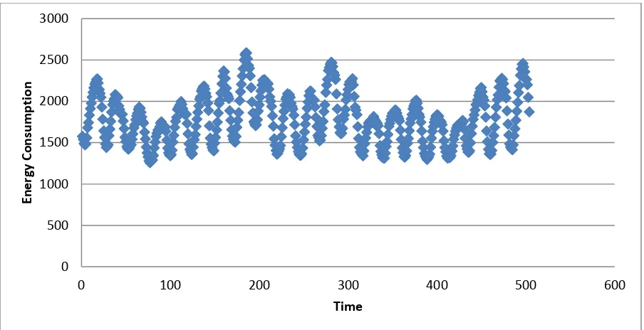
Figure 3.6 - Energy Consumption Demand ... 71
Figure 3.7 - Motifs used in Naïve approach ... 73
Figure 3.8 - Motif Centroid values for Fractured Approach ... 77
Figure 4.1 - Correlated bivariate data ... 87
Figure 4.2A - Intermittent Motif A used in Test Sets ... 103
Figure 4.2C - Block Motif C used in Test Sets ... 105
Figure 4.2D - Intermittent Motif D used in Test Sets ... 106
Figure 4.2E - Intermittent Motif E used in Test Sets ... 107
Figure 4.2F - Intermittent Motif F used in Test Sets ... 108
Figure 4.3A - Test set examples of C1 for Variable 1. Motif A is in red, Motif B in green. 109 Figure 4.3B - Test set examples of C1 for Variable 2. Motif A is in red, Motif B in green. 110 Figure 4.3C - Test set examples of C1 for Variable 3. Motif A is in red, Motif B in green. 110 Figure 4.4 - Intermittent BU Motif ... 111
Figure 5.1 - Motifs created for use in feature space clustering ... 127
Figure 5.2 - Motifs created for use in feature space clustering ... 129
Figure 5.3 - Motifs created for use in feature space clustering ... 134
Figure 5.4 - Motifs created for use in feature space clustering ... 137
Figure 6.1 - Two motifs with overlapping structure for a time series T ... 141
CHAPTER 1: INTRODUCTION 1.1 Introduction and Background
Clustering has become a topic in the forefront of data mining and data analysis. Clustering/classification has touched nearly every aspect of research, from analyzing precancerous lesions (Acosta-Mesa et al., 2014), to music classification (Fu et al., 2011b; Goulart, Guido, and Maciel, 2012), to early prediction of failure in wind turbines (Hoell and Omenzetter 2015; Qiu et al., 2012). Identifying structure in unlabeled data, clustering algorithms are utilized for attribute creation in hierarchical modeling, early warning detection, text analysis, and countless other applications (Chaovalitwongse et al., 2003; Liao, 2005).
Static data clustering methods have been investigated in depth over the course of the past half century. Partitioning clustering algorithms such as k-means which were developed nearly 40 years ago are now implemented into standard software packages with great usage in the scientific and business community (Kabacoff, 2014; SAS, 2015). Density based and hierarchical clustering practices have also become standard fare in the approach towards static clustering (Hennig, 2014).
determining similarity between time series were created to generalize this approach for common data concerns (Moller-Levet et al., 2005). Dynamic Time Warping was created to address speed varying signals (Chan, Fu, and Yu, 2003; Jeong, S., M. Jeong, and Omitaomu, 2011). Strength of signal concerns lead to construction of shapelet and wavelet based
algorithms (Chan et al., 2003; Ye and Keogh, 2011). Alternative similarity measures, using cross-correlation and goodness of fit, were created (Kumar and Patel, 2007; Liao, 2005). A comprehensive survey of previous approaches is given by Tak-chung Fu (Fu, 2011a).
During the course of the development of these time series clustering approaches, a secondary set of approaches was created based upon the alternative assumption that not all data in a time series was of equal worth. In some data cases, periods of relative noise are interrupted with signal, an indication of actors, or sub-processes, acting upon the variable of interest. This inconsistent signal can be seen in many natural processes such as punctuated equilibrium (Gould, 2007). Indeed, even in our daily lives, times of relative banality are broken with points of great interest. This new assumption of time series data structure produced the sub-field of subsequence-based time series clustering.
of actors on a system. An example of this, which is examined further in Chapter 5, is the effect of mixed marketing on sales of retail goods.
Similar to the explosion of different techniques which were created for full time series analysis, many methods were created for evaluation of similarity between
subsequences and the determination of common patterns within time series, known as motifs. Approaches denoted bag-of-words (BOW), or bag-of-features, were created to address the time series data case in which the motifs were known or assumed, in which only
classification of a subsequence as being similar to a motif was required to complete the analysis (Baydogan et al., 2013; Fu et al., 2011b). New similarity functions were created to assist with classification, such as radial distribution functions (Denton, Besemann, and Dorr, 2009). BOW classification strategies were expanded past character and numeric based evaluation, to image classification (Nowak, Jurie, and Triggs, 2006). These methods were useful in situations where motifs were previously known, such as word recognition for text analytics, but lacked the ability to discover new and unexpected motifs.
Motif discovery based algorithms became a popular topic of research to address cases of time series data sets with low prior knowledge. Generation of motifs for use in a bag-of-words approach produced a variety of algorithms (Abdulla_Al_Maruf, and Hung-Hsuan, 2012; Chen, Bi, and Wang 2006; Jadhav et al., 2013; Morrill 1998). A new similarity
encode each subsequence separately. The objective of maximal reduction in overall description length of a time series is the driver for the minimum description length (MDL) approach to subsequence clustering. A greedy iterative approach using this MDL objective was recently created to merge similar subsequences into new motifs, and add membership to pre-existing motifs (Rakthanmanon et al., 2012). This MDL principle has begun to be used in the subsequence clustering community (Mueen et al., 2010; Stine, 2004; Zolhavarieh, Aghabozorgi, and Teh, 2014). A comprehensive discussion of subsequence time series clustering is discussed in Zolhavarieh’s review (Zolhavarieh, Aghabozorgi, and Teh, 2014).
Subsequence based methods have inherent hardships. High memory/computation is necessary to consider all available subsequences in motif discovery algorithms. Noisy data sources can have repeated patterns as a result of chance rather than true signal, leading to spurious results. Restrictive motif structure assumptions can prevent true subsequence signal from being identified in some cases, causing some to find the results of these subsequence clustering approaches meaningless (Keogh, and Lin, 2005; Zolhavarieh, Aghabozorgi, and Teh, 2014).
For all these short-comings, subsequence analysis is still progressing with great interest. The internet of things is fast becoming the new benchmark on which data mining algorithms are tested (Zheng et al., 2011). Device monitoring data comes in with such a high rate that memory storage for entire time series is no longer possible (Sanniano, De Falco, and De Pietro 2014; Silva et al., 2013). Subsequence motifs allow for partial data sets to be kept, with summary tables of occurrences of motifs for time series to be tabulated, reducing
reduce the complexity of computation associated with subsequence analysis (Lian, and Chen, 2008; Nguyen, Ng, and Woon, 2014). As a result of this market need, many packages have been created to address the issue of time series data stream clustering (Pereira and De Mello, 2014; Silva et al., 2013).
Multiple data sources can add to the complexity of data stream analysis. The issue of multivariate data is not a new one. In raw data time series analysis, cross-sectional
approaches were used to address this issue (Kosmelj and Batagelj,1990). In subsequence clustering, univariate studies continue to be the focus, analyzing multivariate time series using univariate clustering techniques on each variable separately. The resultant multivariate time series analysis is created from the compilation, or “stacking”, of these univariate results
(Alonso et al. 2008; Liao 2005). This stacking lacks allowance for interplay between variables in a multivariate time series analysis, resulting in an incomplete understanding of the underlying sub-processes.
1.2 Overview of Dissertation
This dissertation presents and demonstrates a subsequence-based approach to time series clustering, allowing for the flexibility of motif creation with the computational
efficiency of bag-of-words subsequence membership identification, utilizing goodness of fit measures with stochastically defined motifs. The relative occurrence rate of motifs for each time series serves as a feature space, allowing for static clustering methods such as hard k-means, fuzzy c-k-means, and Gath-Geva to be utilized to group similar time series.
to create quick subsequence membership updates, satisfying the growing needs of time series data streams.
The presented approach initially utilizes motif discovery on full time series data through an MDL-based greedy iterative approach, similar to that created by Rakthanmanon et al. (2012). Improvement on the subsequence cluster merging methodology removes redundant clusters. Additionally, this modification allows for subsequence clusters with partially representative patterns to transfer membership to the full pattern subsequence clusters. Business user defined motifs are added prior to the MDL approach, allowing for hypothesized motifs to be included in the MDL process, reducing the considerable
computational time associated with motif discovery.
Completion of the motif discovery phase initializes the creation of stochastic model representations of the subsequence patterns. Multiple approaches to stochastic model
creation are discussed in Chapters 2 and 4, to cover some of the diverse data cases which can occur. After stochastic process estimation, candidate subsequences are able to be evaluated based upon chi-squared or F-like tests, adding/removing membership with much greater speed than allowable via the MDL-based evaluation method of bitsave. The approach is discussed in detail and tested in Chapter 2, with multiple applications demonstrating the effectiveness of this procedure given in Chapter 3.
definitions of the structure of a multivariate motif. A hybrid approach between these two methods is reached, allowing for a linear increase in computational complexity relative to the number of variables to be reached in motif discovery, and a low-cost, higher accuracy
definition of motif to be utilized for incremental loads and/or data streams. This approach has lower computational complexity associated with stacking univariate results, and allows for the interplay of multiple dimensions to define a motif. Real world multivariate
applications are discussed in Chapter 5.
1.3 Extensions to Current Field
The approach outlined in this dissertation extends the current research in a number of ways. Previous work on subsequence clustering has been focused on determining underlying patterns within a single time series, with little research into usage of the relative occurrence of these motifs as a feature space to cluster similar time series together. Additionally, defining motifs by stochastic processes allow for a greater comprehension of the underlying processes and assists in the production of low-cost similarity measures such as chi-square goodness if fit and F-like tests which reduce computation time and allow user-defined similarity thresholds for membership evaluation.
The approach discussed in Chapter 4 expands upon the notion of motifs to include multivariate motif definitions, a concept not extensively researched in the subsequence-based time series clustering literature. Generalization of the definition of a motif to include
CHAPTER 2: UNIVARIATE SUBSEQUENCE-BASED TIME SERIES CLUSTERING
2.1 Introduction
Time series analysis is a topic of great interest across industries. An unprecedented level of time series information is being gathered and analyzed, from process information in manufacturing plants, to point of sales data in retail. In an effort to gain knowledge from these temporal data sets, much work has been put into machine learning and clustering (Liao 2005). As discussed in Chapter 1, two families of approaches to time series clustering have emerged: the first clustering using the entire time series for analysis (Fourier Transforms, Wavelets, etc.), and the second clustering occurrences of common subsequences within a series (Bag-of-Words, MDL-based motif discovery) (Liao, 2005; Lin et al., 2007).
Continual monitoring systems have recently become a topic of great interest, in which time stamped data streams produce time series too large for full storage (Zheng et al., 2011). This business need to not retain full time series information has created a heightened interest in subsequence-based time series clustering. This chapter outlines a comprehensive
univariate subsequence-based approach to time series clustering.
The first issue of subsequence clustering can be addressed with one of two
approaches: user defined motifs, or motif creation through discovery (Baydogan et al., 2013; Rakthanmanon et al., 2012). User-defined motifs can be useful, but suffer from the potential for an incomplete set of motifs, as well as the possibility of those motifs being of poor/biased quality. Alternatively, motif discovery creates subsequence clusters from similar
subsequence occurring in the data. The associated motif to this subsequence cluster is equal to the average of the subsequences with membership to the cluster, producing an unbiased pattern occurring in the time series.
The second issue of subsequence clustering is addressed through similarity measures. Euclidean distance, dynamic time warping distance, and description length are just a few of the measures which have been utilized to determine the similarity between two
subsequences, or a subsequence and a motif (Zolhavarieh, Aghabozorgi, and Teh, 2014). One approach to motif discovery uses description length as the basis of a greedy iterative algorithm which minimizes the overall description length of a time series (MDL)
(Rakthanmanon et al., 2012).
Using the natural concept of reduction in description length associated with any creation or update to a subsequence cluster, this iterative algorithm can provide a
comprehensive list of motifs occurring in the data set. A user-defined motif input prior to a MDL-based algorithm will be the basis of the motif creation/discovery portion of the approach outlined in this chapter.
of assumptions, a choice of type of stochastic process is made by the user. Estimation of the parameters associated with the stochastic process is performed to create a hypothesized distribution of the subsequence cluster pattern. This constructed distribution allows for chi-square goodness of fit or F-like tests to be used on eligible subsequences to provide a quick and informative measure of similarity. Given subsequences which are not significantly dissimilar from the hypothesized distribution, using a user-defined threshold for level of significance, these subsequences can be added to the most representative subsequence cluster.
The completion of motif discovery, stochastic process definition/estimation, and membership additions/removals using the goodness of fit similarity measure, allows for the creation of a motif occurrence rates for each time series. Using these motif occurrences as a feature space, a choice of static clustering approaches is selected to group similar time series, completing the full approach.
Section 2.2 discusses all background information necessary for creation of the
subsequence-based time series clustering approach. Section 2.3 explains the methodology of this approach in detail, explaining the process in 5 distinct phases. Additionally, this section discusses incremental updates, in which the value of having the low-cost goodness of fit similarity measure is truly realized. The complexity of each of the phases from Section 2.3 is discussed in Section 2.4.
explanation of the construction of the datasets used for these tests is given in Section 2.5 and the associated clustering results are given in Section 2.6.
2.2 Background and Notation
2.2.1 Minimum Description Length Process Definition 2.1- Time Series/Length
A time series T is a sequence of values 𝑡1, 𝑡2, … , 𝑡𝑛 representing the realization of a variable at each of the n points in time. The length of the time series T is defined as n. Definition 2.2- Subsequence
A subsequence𝑇𝑖,𝑘= 𝑡𝑖, 𝑡𝑖+1, … , 𝑡𝑖+𝑘−1 is a group of values within the ordered sequence T, of length 𝑘 ≤ 𝑛 which is ordered as in T without exclusion. This definition requires 𝑖 ∈ {1,2, … , 𝑛 − 𝑘 + 1}.
A time series is not explicitly required to have an evenly spaced set of observations. However, for the purposes of our study we assume even spacing. Additionally, continuous valued time series data is required to be discretized for the purposes of the MDL algorithm, with values between 1 and 2𝑏. The constant b, defined as the level of resolution, allows for a lossy discretization/normalization of the subsequence data. The purpose of this
discretization/normalization is two-fold. Firstly, the normalization allows for the comparison of two subsequences based on their relative shapes, removing issues of scale. Secondly, the discretization allows for a computation of the number of bits required to encode the
Definition 2.3- Discrete Normalization
Given a continuous valued subsequence T, the discretized sequence representation is produced by the discrete normalization function DNorm, defined as:
𝐷𝑁𝑜𝑟𝑚(𝑇) = 𝑟𝑜𝑢𝑛𝑑 (( 𝑇 − 𝑇𝑚𝑖𝑛
𝑇𝑚𝑎𝑥 − 𝑇𝑚𝑖𝑛) 𝑥(2𝑏− 1)) + 1,
where Tmin and Tmax are the minimum and maximum values of the sequence T. The result of this transformation is that all values fall between 1 and 2𝑏. When Tmax=Tmin,
DNorm(T) will be set to a vector of 2b-1s.
The normalization of subsequences allows for similarity of shape to be assessed. One quick assessment of the similarity of curves for two subsequences of the same length is by the Euclidean norm. While not used for the final membership assessment in this chapter’s approach, the Euclidean distance measure provides a low computational cost method to assess similarity, with results similar to that of using description length (Rakthanmanon et al. 2012).
Definition 2.4-Euclidean Distance
The Euclidean distance between subsequences 𝑇𝑖,𝑘 and 𝑆𝑗,𝑘 is:
𝐸𝐷𝑖𝑠𝑡(𝑇𝑖,𝑘, 𝑆𝑗,𝑘) = √∑(𝑡𝑖+𝑙− 𝑠𝑗+𝑙)2 𝑙−1
𝑙=0
Definition 2.5-Entropy
The entropy of a time series T is defined as follows:
𝐻(𝑇) = − ∑ 𝑃(𝑇 = 𝑡) log2𝑃(𝑇 = 𝑡) , 𝑡
where P(T=t) is the probability that a randomly chosen value in the series T has a value of t, and with the convention that if P(T=t*)=0, then 𝑃(𝑇 = 𝑡 ∗) log2𝑃(𝑇 = 𝑡 ∗) = 0.
If there are a set of subsequences which have a common pattern, then encoding the information of those subsequences by a motif and the associated deviation of the
subsequences from that motif could take up less total memory than encoding each of the subsequences separately. This reduction in encoding memory is caused by a fewer number of bits being required to encode the associated differences rather than the original
subsequences. The entropy can be interpreted as a measure of the amount of memory required to encode each position of a time series. The description length measures the relative amount of memory required to encode the entire series T.
Definition 2.6-Description Length
The description length of a time series T of length n is: 𝐷𝐿(𝑇) = 𝑛 ∗ 𝐻(𝑇)
Definition 2.7- Subsequence Cluster/Motif of Subsequence Cluster
Intuitively, a motif is a repeated pattern in the time series. Motifs need not be defined by a subsequence, but can be defined solely by the pattern, as is the case in bag-of-words approaches. In this case, the motif is not affected by the realizations of the associated subsequences, which allows for subsequences to deviate from the motif in a biased manner. These business-user-defined motifs are discussed further in Section 2.3.1.
Definition 2.8-Conditional Description length
The conditional description length of a subsequence B associated a motif H is: 𝐷𝐿(𝐵|𝐻) = 𝐷𝐿(𝐵 − 𝐻)
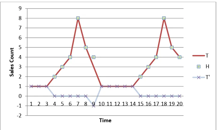
Figure 2.1 - T is partly represented by the motif H to produce T’
Using conditional description length definition, the usefulness of a motif becomes clearer. As an example, Figure 2.1 displays the time series T of the number of car sales over the course of 20 weeks. T4,6 and T15,6 display a near exactly recurrent subsequence pattern.
-2 -1 0 1 2 3 4 5 6 7 8 9
1 2 3 4 5 6 7 8 9 10 11 12 13 14 15 16 17 18 19 20
Sal
e
s
Co
u
n
t
Time
Creating a subsequence cluster CH={T4,6, T15,6} results in the motif H=2, 3, 4, 8, 5, 4 (rounding to nearest integer).
The time series can be modified by the subsequence cluster CH. T’ is the resultant series, taking the difference of T and H for T4,6 and T15,6. For notation,
𝑇’ ∶= (𝑇|𝐻) = {𝑇 − 𝐻, 𝑓𝑜𝑟 𝑠𝑡𝑎𝑟𝑡𝑖𝑛𝑔 𝑝𝑜𝑖𝑛𝑡𝑠 𝑡 = {4,15}𝑇, 𝑜𝑡ℎ𝑒𝑟𝑤𝑖𝑠𝑒
Examining T’ in Figure 2.1, there are fewer realized values in T’. As a result, it is possible to encode T’ into memory using fewer bits, measured by a lower resultant
description length. Calculating the description lengths:
DL(T)=20*.70635=14.127, DL(T’)=DL(T|H)=20*.36703=7.341, DL(H)=6*.67781=4.067
The original description length for T is 14.127. Using subsequence cluster CH to reduce the entropy of T, T’ has a description length of only 7.341! There is the additional
cost of the description length for H of 4.067, producing a total description length of encoding T using CH of 11.408. The MDL approach seeks to minimize the total description length of a time series T by using subsequence clusters. As a result, MDL would determine the motif H defined by CH to be a significant pattern within the series T, and CH would be utilized. Definition 2.9-Description Length of a Cluster (DLC)
The description length of a cluster CH with centroid H and members 𝐴 ∈ 𝐶𝐻 is:
𝐷𝐿𝐶(𝐶𝐻) = 𝐷𝐿(𝐻) + ∑ 𝐷𝐿(𝐴|𝐻) 𝐴∈𝐶
clusters associated utilized by a time series T. Three actions can be performed on the set of subsequence clusters. These actions are forming a new subsequence cluster defined by two subsequences in T, adding a subsequence of T to a preexisting cluster, or merging the membership sets of two clusters together. Each of these actions alters the description length of T, and the extent of the change is defined by the bitsave.
Definition 2.10-Bitsave
The bitsave associated with an action on the set of subsequence clusters is the difference in the description length of T before versus after the action is used. Namely,
𝑏𝑖𝑡𝑠𝑎𝑣𝑒 = 𝐷𝐿(𝑇|𝐶𝑙𝑢𝑠𝑡𝑒𝑟𝑠 𝑏𝑒𝑓𝑜𝑟𝑒 𝑎𝑐𝑡𝑖𝑜𝑛) − 𝐷𝐿(𝑇|𝐶𝑙𝑢𝑠𝑡𝑒𝑟𝑠 𝑎𝑓𝑡𝑒𝑟 𝑎𝑐𝑡𝑖𝑜𝑛)
An action with positive bitsave reduces the description length of T and is a candidate for use. The greedy approach to MDL chooses the action with the greatest bitsave, and if the associated bitsave is positive, uses this action upon the set of subsequence clusters. A
detailed discussion of the actions available is given in Section 2.3.
This subsection gave the framework required for motif discovery and refinement. As discussed further in Section 2.3.4, the members of the subsequence clusters can be
2.2.2 Poisson Processes Definition 2.11-Poisson Distribution (X~Pois(𝜆))
A discrete random variable X has a Poisson distribution with occurrence rate 𝜆 if it takes on values of nonnegative integers k=0,1,2,… with probability function:
𝑓(𝑘, 𝜆) = Pr(𝑋 = 𝑘) =𝜆 𝑘𝑒−𝜆
𝑘!
Definition 2.12-Time Homogeneous Poisson Process
A Time Homogeneous Poisson process, N(t), is a stochastic counting process of the number of occurrences of an event within the time span (0,t], in which the time between occurrences, X, is exponentially distributed with parameter 𝜆. The probability of k occurrences between times t and t+h follows a Poisson distribution with occurrence rate 𝜆ℎ. Namely,
𝑃[𝑁(𝑡 + ℎ) − 𝑁(𝑡) = 𝑘] =𝜆ℎ 𝑘𝑒−𝜆ℎ
𝑘!
In order for a counting process N(t) to be a Time Homogeneous Poisson, only 4 assumptions need to be satisfied (Varahan, 2000):
i) For every h>0, the distribution of N(t+h)-N(t) is the same for every t>0 (the time homogeneity assumption).
ii) If (a,b] and (c,d] do not overlap, then the random variables N(b)-N(a) and N(d)-N(c) are mutually independent (Memory-less).
iii) N(0)=0, N(t) integer valued, right continuous, non-decreasing in t with probability equal to 1 (Properties of a counting process).
For a counting process in many industry functions, (iii) is applicable if negative counts are not allowed or are negligible (e.g. returns of merchandise). Assumption (iv) is also often reasonable, given events which do not occur densely. Note that there can be occurrences in which multiple events occur at the same time, but if they are rare it is possible to model them as being a small distance apart, especially when looking at time aggregated data.
In some cases it may be that the counting process is dependent on time. In these cases assumption (i) is not satisfied and the result is a time nonhomogeneous Poisson process. Definition 2.13-Time Nonhomogeneous Poisson Process (NHPP)
A Time Nonhomogeneous Poisson process (NHPP), N(t), is a Poisson process in which the occurrence rate 𝜆 now varies with time. Define the occurrence rate as 𝜆(𝑡), and the occurrence rate over the interval t=(a,b] as:
Λ𝑎,𝑏= ∫ 𝜆(𝑡)𝑑𝑡𝑏 𝑎
The NHPP has the property that the likelihood of k occurrences in the interval t=(a,b] has a Poisson distribution with occurrence rate Λ𝑎,𝑏:
𝑃[𝑁(𝑡 + ℎ) − 𝑁(𝑡) = 𝑘] =Λ𝑎,𝑏
𝑘𝑒−Λ𝑎,𝑏
𝑘!
2.2.3 Gaussian Processes
Definition 2.14-Gaussian Distribution (𝑋~𝑁(𝜇, 𝜎2) ) (Gallager 2013)
𝑓𝑋(𝑥) = 1 √2𝜋𝜎𝑒
−(𝑥−𝜇)2
2𝜎2
Definition 2.15-Gaussian Process (Gallager 2013)
A Gaussian process {X(t);t ϵT} is a stochastic process such that for any set of k time epochs, t1, …, tk ϵ T, the set of random variables X(t1),… , X(tk) is a jointly-Gaussian set of random variables.
2.3 Methodology
The approach outlined in this section provides a comprehensive end-to-end approach to subsequence-based time series clustering. The approach is broken into five phases, each of which addresses a particular concern inherent in time series clustering. Phase 0 allows for the input of defined motifs with levels of confidence in the motif chosen. These user-defined motifs create artificial subsequence clusters. Phase 1, the first MDL-based motif discovery phase, acts upon the time series, creating new subsequence clusters in addition to the user defined motifs, and adding membership to preexisting subsequence clusters. Phase 2 Part 1 merges subsequence clusters together, creating new candidate subsequence clusters. At this point, the MDL-based approach laid out in Rakthanmanon’s work is completed. Additional steps beyond Rakthanmanon’s work are given in Phases 2 Part 2, 3, and 4.
Discussed in Section 2.3.3.2, the subsequence cluster merging in Phase 2 Part 1 can produce motifs not naturally occurring in the data. To combat these bad motifs, and to reduce the set of clusters to only those with distinct motifs, Phase 2 Part 2 reevaluates
3 creates stochastic models for each subsequence cluster of sufficient size, using the membership subsequences as realizations of the process. These stochastic models create hypothesized distributions on which dissimilarity can be assessed, using chi-square goodness of fit or an F-like test statistic, for new eligible subsequences.
Phase 4 accumulates the relative subsequence membership rates for each time series being considered, and uses these rates as a feature space. Partition clustering is performed on this feature space to create groupings of similar time series. Pseudocode for this approach is given in Appendix A.
This algorithm is customizable to fit the needs of a particular data set. The parameters available for modification are:
1. The motif window [MMmin, MMmax].
2. Iteration cutoffs for Phases 1 and 2 Part 2 (used in the case of time restrictions). 3. The minimum subsequence cluster size to be considered for stochastic modeling
in Phase 3.
4. The threshold for the dissimilarity required for a subsequence to not become a member of a subsequence cluster, used in the goodness of fit test (alpha level).
5. The maximum number of series clusters to be used in Phase 4.
6. The partition clustering algorithm to be used on the subsequence cluster occurrence feature space in Phase 4.
discovered by subsequence clusters, realized through multiple distinct subsequence clusters as is demonstrated in Section 2.6.
2.3.1 Phase 0: Business User Input
Unsupervised machine learning has many attributes to its benefit. It is attractive to think about an algorithm which can be applied to an arbitrary set of time series data,
information gathered without any prior knowledge or hypotheses, the results of this approach creating meaningful knowledge which drives innovation and discovery. There are two criticisms to the unsupervised learning approach. The first is that there may be false artifacts, patterns found in the noise, which appear to be significant. When chosen, these erroneous motifs can stifle the learning process, especially with an exclusionary greedy algorithm such as MDL. The second criticism to the automated approach is that a data set is rarely
unknown. In many business cases, the variable of interest in a time series is accompanied with expert theories on the sub-processes acting upon the variable of interest and potential patterns which can occur. In Phase 0, these theories are used to create initial guesses at behaviors expected to be occurring in the data, through defined motifs. These user-defined motifs are assessed in Phases 1 and 2, adding subsequences to membership as
appropriate. If there is sufficient subsequence membership at the end of Phase 2, a stochastic process representation of this motif is created in Phase 3, and the motif occurrence rate is used in Phase 4. Usage of user-defined motifs addresses some of the criticisms associated with automated motif discovery, and leads to increased speed in Phases 1 and 2.
subsequence cluster with the associated user defined motif. Another way to describe this approach is that given a confidence level of x, x artificial subsequences equal to the motif are created and given membership to the cluster. A lower size (1 or 2) allows for a greater level of adjustment from the real data to account for inaccuracies than would be possible with a size of 1000. Indeed, due to the rounding and normalization occurring after each action in Phase 1, placing a sizing of greater than 2b-3 ensures that the motif does not change, where b is the level of resolution.
2.3.2 Phase 1-MDL Cluster Creation
Given the initialization of user-defined clusters (motifs along with associated confidence sizing), the modified MDL algorithm begins. As stated in Section 2.2, the concept underlying MDL is minimizing the amount of memory (description length) required to describe the time series. Description length is reduced iteratively, choosing an action with the greatest positive bitsave to use upon the set of subsequence clusters. In Phase 1, two actions are possible for use, a modification of the approach by Rakthanmanon et al. (2012). Action 1: The merging of two subsequences-
Two subsequences of the same length create the membership set of a subsequence cluster with motif (centroid) equal to the average of these two subsequences. There is an associated subsequence cluster size of 2 (each subsequence unto itself is
considered to have a size of 1 and size is additive).
If CH is previously of size x, length n, and motif M=m1, m2, …, mn, the addition of subsequence Ti,n=ti,1, ti,2,…,ti,n, updates CH to a cluster of size x+1, with centroid M’=(xM+ Ti,n)/(x+1).
For a subsequence to be considered for these actions, no portion can have previously been assigned membership (no overlapping subsequences). A subsequence which does not have any data points with membership to subsequence clusters is denoted actionable, or eligible. At each iteration of the MDL algorithm, the two nearest actionable subsequences are found using the low-cost Euclidean distance metric, for each length L in the motif window. The bitsave associated with Action 1 on these subsequences is calculated and stored for review. For each cluster, the nearest actionable subsequence is also selected using the Euclidean distance. The bitsave associated with Action 2 on this subsequence and cluster is assessed and stored for review.
Upon completion of all bitsave calculations, the action with the largest bitsave is chosen. If the bitsave is positive (a reduction in the overall description length of the data), then the associated action is completed. Eligibility of actionable subsequences is reassessed after the update to the set of subsequence clusters, and the next iteration begins. These iterations continue until the greatest bitsave is negative, or the maximum number of iterations possible is reached. The setting of maximum number of iterations is solely for the purpose of time consideration.
similar motifs, but does give preference to Action 2 over Action 1, given the same bitsave. In order to compress similar clusters, Phase 2 allows for usage of the third action: merging membership sets of similar clusters.
2.3.3 Phase 2-Cluster Pruning 2.3.3.1 Phase 2 Part 1-Merging similar clusters
Phase 1 produces a set of subsequence clusters, some of which may lack distinctness, or overlap significantly with another cluster within the set. To remedy these issues, a third action is created: merging two clusters together. This action is defined in a similar bitsave framework to the first two actions.
Action 3: Merging of two clusters-
Given two subsequence clusters C1 and C2, with lengths Li, sizes Si, motifs 𝑀𝑖,𝐿𝑖, and
an offset Oi, the resultant cluster C3 has size S1+S2, length L3=max(L1+O1,L2+O2), and motif:
𝑚3,𝑗 =
{
𝑆1𝑚1,𝑗−𝑂1+ 𝑆2𝑚2,𝑗−𝑂2
𝑆1+ 𝑆2 , 𝑖𝑓 𝑂1 < 𝑗, 𝑂2 < 𝑗, (𝑗 − 𝑂𝑖 ) ≤ 𝐿𝑖 𝑚1,𝑗−𝑂1, 𝑖𝑓 𝑂1 < 𝑗, 𝑂2 ≥ 𝑗, (𝑗 − 𝑂1 ) ≤ 𝐿1
𝑚1,𝑗−𝑂1, 𝑖𝑓 (𝑗 − 𝑂1 ) ≤ 𝐿1, 𝑂2+ 𝐿2 < 𝑗
𝑚2,𝑗−𝑂2, 𝑖𝑓 𝑂2 < 𝑗, 𝑂1 ≥ 𝑗 , (𝑗 − 𝑂2 ) ≤ 𝐿2 𝑚2,𝑗−𝑂2, 𝑖𝑓 (𝑗 − 𝑂2 ) ≤ 𝐿2, 𝑂1+ 𝐿1 < 𝑗
,
Given the constraints on motif length, the overlaps Oi are restricted such that L3 is within the motif window. In order to assess the bitsave associated with this merger, the difference of each subsequence associated with either motif cluster is calculated, based on the relevant portion of M3. The description length prior to Action 3 is 𝐷𝐿𝐶(𝐶1) + 𝐷𝐿𝐶(𝐶2). The new description length 𝐷𝐿𝐶(𝐶3) is calculated under the caveat that the conditional description lengths of the subsequence members use only the applicable portion of M3. The bitsave of merging two similar clusters together is positive when there is high similarity of members along that overlap. In these cases, the increased conditional description costs associated with changing the motif value along the overlay is offset by the reduced description length of motif M3 as compared to that of M1 and M2.
There is the potential for erroneous clusters to be created using Action 3. The bitsave calculation described above, based on the approach by Rakthanmanon et al., does not check to determine if the entire motif M3 occurs in the dataset. Indeed, it is possible that M3 can be produced from a partial overlap of M1 and M2, with no difference in overlaid values, and M3 never occurs within the time series data.
Figure 2.2A - Two motifs from Phase 1. S1=5, S2=8, O1=0, O2=0
Figure 2.2B - Offset second cluster. O2=3 0
2 4 6 8 10 12
0 2 4 6 8 10
M1 M2
0 2 4 6 8 10 12
0 2 4 6 8 10 12
Figure 2.2C - M3 created from M1 and M2 with O1=0, O2=3
Figure 2.3A - Time series T with associated motif cluster A and B membership shown 0
2 4 6 8 10 12
0 2 4 6 8 10 12
0 2 4 6 8 10 12 14 16
0 5 10 15 20 25 30 35 40 45
Figure 2.3B - M3 made from Highest Bitsave associated Action 3 (O1=0, O2=3)
Unfortunately, Action 3 does not always produce a cluster with a motif that actually occurs in the time series data. It does always produce a candidate cluster which has a length larger than or equal to each of the initial clusters and a good motif representation of member subsequences on the overlap. As a result, if subsequences do occur naturally with this motif, representing those subsequences by this amalgamated cluster can reduce description length. Phase 2 Part 2 was created to determine which of these new motifs occur in the data.
In order to determine all candidate clusters which may be represented in the data, an iterative approach to merging clusters is taken in Phase 2 Part 1. Beginning with all clusters from Phase 1 being set to active, the maximum bitsave of action 3 of each merger is assessed (varying on the offsets). The largest bitsave associated with Action 3 across all pairings is determined, and if positive, that instance of Action 3 is taken. Without loss of generality, let C1 and C2 be the clusters on which Action 3 is carried out, with the resultant cluster denoted C3. C3 is set to active, with cluster size equal to the sum of the sizes of C1 and C2. The
0 2 4 6 8 10 12
merger size of C3, denoted MS3, is defined to be the number of clusters from Phase 1 which were merged to create C3. Therefore MS3= MS1+MS2, using the convention that any subsequence clusters from Phase 1 have MSi=1. C1 and C2 are then set to inactive to complete the iteration. This process iterates on active clusters until there is not a positive bitsave associated with any instances of Action 3, or there is only one active cluster. The output of this phase is a list of all subsequence clusters.
2.3.3.2 Phase 2 Part 2-Reselecting Subsequence Membership
Phases 1 and 2 Part 1 produced a plethora of candidate subsequence clusters. Phase 2 Part 2 reduces the overall number of subsequence clusters, determining which distinct
clusters are represented in the time series data. Facilitating this reduction of clusters requires subsequence membership be reassessed. For each subsequence cluster CH resultant from Phases 0 to 2 Part 1, the associated motif H is used to create an artificial subsequence cluster CH,A, with a confidence level/cluster size of 2b-3. Let the merger size transfer from CH to C-H,A. Membership to all subsequence clusters are rescinded, making every subsequence
eligible for membership to the artificial subsequence clusters. These artificial clusters are used to recreate membership levels.
greatest bitsave is negative, or maximum number of iterations is achieved (set by user, based on time constraints).
Upon termination of the iterative process for all artificial clusters with motif size equal to MSmax, the iteration count is reset to 1 and Action 2 is allowed only on artificial clusters with motif size equal to MSmax-1. Using this new set of actionable clusters, the same iterative process is run until termination. This process is repeated, each time decreasing the motif size by 1, until all clusters have been actionable.
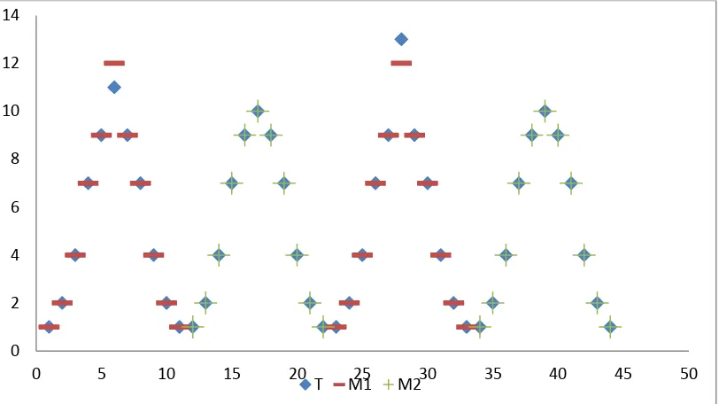
What does this process do? It allows for subsequence membership testing on those merged clusters to ensure that the associated motifs do occur in the time series data. In addition, for those Phase 1 clusters which have similar motifs and the same length, a cluster created in Phase 2 Part 1 composed from those two clusters, with full overlap, will be populated with the memberships of both Phase 1 clusters, leaving no eligible subsequences remaining for the Phase 1 clusters at the last stage of the phase. A minimum cluster size threshold in Phase 3 will remove low count subsequence clusters from consideration, thus replacing the two Phase 1 clusters in the above example with the Phase 2 Part 1 candidate cluster. An example of the usefulness of this multi-stage approach is given in Figure 2.4.
Figure 2.4 - T with associated motifs M1 and M2 overlaid at end of Phase 1
At the completion of Phase 2 Part 2, the members of the artificial clusters are used to recreate the subsequence clusters and associated motifs. Any clusters which have size less than a user defined threshold will be removed at the beginning of Phase 3, with the remaining representative clusters modeled by stochastic processes.
2.3.4 Phase 3-Stochastic Process Estimation
The motif discovery portion of the approach is now completed. All subsequence clusters which have size greater than the user defined threshold have associated motifs which occur frequently within the time series and are distinct. Each of these motifs can be thought of as a stochastic sub-process within the time series; each subsequence with membership a realization of that process. As a result, a hypothesized stochastic process can be determined
0 2 4 6 8 10 12 14
0 5 10 15 20 25 30 35 40 45 50
based upon they style of data used in the time series. The parameters of the process are then estimated using the subsequence members.
Counted data motifs may be appropriately represented by Poisson processes (Case 1). Continuous data time series may be approximated with Gaussian processes (Case 2). A third ‘catch all’ case, used in the presence of data not accurately represented by Gaussian or
Poisson processes, is discussed briefly in this section and discussed further in Chapter 4. Phase 3 Case 1-Counted Data
In the case that the time series variable of interest is counted data, motifs may be considered as Poisson processes, with each member of the subsequence cluster a realization of that process (Varahan 2014). If the assumptions (ii) to (iv) are satisfied or nearly satisfied (see Section 2.2.2), Poisson processes can be a useful representation of the motif. Parameter estimation of occurrence rate function 𝜆𝐻(𝑡) is performed using spline approximations for each subsequence cluster CH (Massey, Parker, and Whitt 1996). The function PROC TRANSREG in SAS® is used to perform this spline fitting, using cubic splines (Pedan 2014). The number of knots specified for this spline approach is given by SAS procedure guidelines (Qamar 1993). The variable of interest will be set as having a log linear response relationship with the spline function on time (Lewis, and Shelder 1976).
After creation of the occurrence rate function 𝜆(𝑡) using cubic splines, an F-test is used to determine if the approximation is significantly different from the null hypothesis of a constant occurrence (𝜆(𝑡) = 𝜆). If the F-test evaluates the spline function (Time
significantly different from the null model of an average occurrence rate, a time homogeneous Poisson process will be estimated.
Phase 3 Case 2-Continuous Data
Given continuous time series data, motifs could be defined by Gaussian processes. Given empirical distributions of the member values at each time epoch for a subsequence cluster, the appropriateness of using a Gaussian process can be assessed (Definition 2.14). Mirroring the approach in case 1, cubic splines are used to approximate the progression of the parameters μ and σ through the motif. F tests are used to determine if the μ(t) and σ(t) are significantly different from the constant functions μ(t)= μ and σ(t)= σ.
Phase 3 Case 3-Volatile Data
In some cases the assumptions required for Poisson or Gaussian processes are not satisfied sufficiently, and a generalized approach is used. Additionally, in cases of highly volatile motif patterns, parameter estimation via cubic spline functions or flat models is insufficient to capture the motif’s pattern sufficiently. In such a case, the distribution of each
time epoch of a subsequence cluster is modeled by a stochastic random variable independent of the other time epochs. This case is discussed in detail in Section 4.4.1.
Using one of the previous cases, parameter functions are estimated and a
hypothesized distribution of a motif is produced. A similarity measure can now be used to determine membership of subsequences to each cluster based on these stochastic processes. Two similarity measures are chosen between, dependent on the type of stochastic process defining the motifs: chi-square like goodness-of-fit tests, and F like tests.
The Pearson’s chi-square goodness of fit test provides a statistical similarity measure
for Poisson processes (Case 1). Comparing the number of occurrences at each time epoch of a subsequence to those expected from a Poisson process is used to create the associated chi-square value. Namely, for a subsequence Ti,k and a subsequence cluster C with expected values cj at each time epoch j, the associated chi-square test statistic is:
𝑋2 = ∑(𝑡𝑖+𝑗−1− 𝑐𝑗)2 𝑐𝑗 𝑘
𝑗=1
The usage of goodness of fit tests are to determine if a set of observations differ significantly from a theorized distribution with associated alpha level ɑ. Using a larger alpha level than is normal for these tests (e.g. .3 rather than .01) only subsequences with values very near to the motifs will be defined as not significantly dissimilar from the hypothesized distribution. These subsequences will become members of that cluster.
In Cases 2 and 3, data which does not measure occurrences of an event precludes the use of such a statistical method for explicit statistical interpretation. In many applications however, variables of interest which are not explicitly counted data can still have the
While no statistical interpretation of the chi-square test statistic may be possible for this case, the pseudo p-value created does provide an accurate comparison measure for determining the relative distance of a subsequence to candidate subsequence clusters. Using a defined alpha level as a cutoff threshold, this pseudo p-value can also be used to determine membership of a subsequence to a subsequence cluster.
Similarity measure 2: F-Like Test
The chi-square goodness of fit test is a useful similarity measure when considering Poisson processes, but for many variables of interest this method is not appropriate. An F-like statistic can be created to measure the deviation of a subsequence from a stochastic process, using the associated expected variance of the process at each time epoch as a weighting factor, rather than the mean as was used in the chi-square like test statistic.
For subsequence Ti,k and a subsequence cluster C with length k and an associated stochastic process which has expected values μi and variances 𝜎̂2𝑖 at each time epoch i, the F-like statistic is:
𝐹 =∑ (𝑡𝑖+𝑗−1− 𝑐𝑗) 2 𝑘
𝑗=1
∑ 𝜎̂2 𝑗 𝑘 𝑗=1
,
For the sake of convenience, references to significance of dissimilarity or hypothesis testing will assume Case 1 data, with equivalent alpha level threshold comparisons to pseudo p-values performed for data which do not use Poisson processes for motif definition.
Using the appropriate similarity measure, current members of each subsequence cluster are evaluated, removing subsequences sufficiently dissimilar from the motif. After removing these dissimilar members, eligible subsequences are evaluated against each
candidate motif of the same length. If a subsequence has at least one test which fails to reject the null hypothesis, this subsequence will be considered for membership to the subsequence cluster with the least dissimilarity.
A greedy iterative approach is used to select the least dissimilar subsequence/cluster pairing, assigning membership and setting all overlapping subsequences to ineligible if at least one subsequence/cluster pairing resulted in similarity measure which failed to reject the null hypothesis. This process is repeated until there are no remaining eligible subsequences with this property.
2.3.5 Phase 4-Frequency Analysis and Similarity of Time Series Subsequence memberships have now been assigned to each stochastic process defined subsequence cluster. For each time series, relative membership frequency to each subsequence cluster create a z-dimensional space (z=number of clusters post-Phase 3 with membership greater than some predefined threshold). A multidimensional clustering
The hard k-means clustering approach, a deterministic, Euclidean similarity measure, partition clustering approach will be used extensively in the examples given in chapters 3 and 5 (Rogers et al., 2012). Alternatively, Fuzzy C-Means, or Gath-Geva are also available for use and are preferable when there are highly different variances in the occurrence rate for the motifs (Miyamoto et al., 2008; Dumitrescu et al., 2000).
These partitions represent similar time series based on the sub-processes which act upon them. This approach provides a comprehensive subsequence-based clustering tool, providing not only the clustering for an initial set of time series, but also the motif framework for quick, low computational cost updates to these time series feature spaces. Additionally, new time series can be evaluated in short order.
2.3.6 Incremental Updates (Full and Partial)
Time series for in-process systems are not static, but require reevaluation as more data arrives. Further, a system may not be closed, with additional time series entering the set of series to be evaluated. This is exemplified in retail by new products being introduced to a store, and additional point of sales information becoming available as time progresses. In data streaming, monitor data flows in with such fluidity that storage of the entire time series is cost-prohibitive. A modified update structure using the appropriate similarity measure (see Section 2.3.4) provides a low cost subsequence cluster membership, allowing for updates to the relative motif occurrence rates as information pours in.
upper bound. As a result, the benefit to performing the full 5 phase approach lessens as the set of subsequence clusters encapsulates more of the sub-processes.
2.3.6.1 Partial Update
In a partial update, new membership is assessed for any new subsequences which have not been evaluated in previous steps. Using the previously estimated stochastic processes associated with motifs, the associate similarity measure tests (chi-square like or F-like) are run against the new data. A list of all eligible subsequences which had at least one test that failed to reject the null hypothesis is compiled. Using the greedy iterative algorithm, the least dissimilar subsequence will be given membership to the associated cluster, updating the list of eligible subsequences to remove those subsequences which have overlap. This process continues until the list is empty.
The feature space of relative motif occurrence is updated to reflect the new
memberships and partition clustering is run to reevaluate similarity. This process requires low computational cost. If a fuzzy clustering approach is used, keeping archived snapshots of the feature space can provide insight into shifts in groups of time series, providing additional information about changes in the factors acting upon the time series. 2.3.6.2 Full update
streams, a data stream collection process will occur periodically to retain a larger interval of data for full update purposes. Upon completion of the full update, this larger time series interval is removed from memory and the new/updated stochastic processes are used for incremental updates.
2.4. Speed and Complexity
Complexity of Actions 1-3 as well as Phase 1 are outlined in Rakthanmanon’s paper on MDL-based clustering (Rakthanmanon, 2012). Let the amount of effort in evaluating the best options for Actions 1 to 3 on a specific instance be N1, N2, and N3 respectively.
2.4.1 Phase 2 Part 1
Given k motif clusters from Phase 1, there will be one iteration of k(k-1)/2 evaluations of each cluster pairing. The amount of effort required for merging two
subsequence clusters and evaluating the bitsave associated Action 3 is N3. In the worst case that two clusters of minimal motif length, there are 2(MMmax-MMmin)+1 potential offsets, each of which have a cost of N3. Therefore the first iteration of Phase 2 Part 1takes uses k(k-1)/2*(2(MMmax-MMmin)+1)*N3 effort in the worst case.
At iteration i>1 there are k-i+1 available clusters for comparisons, and only one cluster which has not been compared to each of the previous clusters. There are k-i cluster pairings considered in this iteration, each of which have 2(MMmax-MMmin)+1 potential offsets requiring N3 effort. The total worst case effort for iteration i>1 is:
(k-i)*(2(MMmax-MMmin)+1)*N3.
2.4.2 Phase 2 Part 2
Suppose k2 candidate clusters result from Phase 2 Part 1. These are added to the k clusters from Phase 1, such that:
𝑎𝑗 = # 𝑜𝑓 𝑐𝑙𝑢𝑠𝑡𝑒𝑟𝑠 𝑤𝑖𝑡ℎ 𝑚𝑒𝑟𝑔𝑒𝑟 𝑠𝑖𝑧𝑒 𝑗
For j=1 to MSmax, each j-level can have up to a user defined threshold of iterations, MAXITERP2. Each iteration requires up to aj evaluations of Action 2. Therefore the effort for Phase 2 is bounded above by:
∑ 𝑎𝑗∗ 𝑁2∗ 𝑀𝐴𝑋𝐼𝑇𝐸𝑅𝑃2 𝑀𝑆𝑚𝑎𝑥
𝑗=1
2.4.3 Phase 3
Given k3 motif clusters CI resulting from Phase 2 with sufficient size Si, a stochastic process is fitted. The SAS package for these functions is quick, with an effort of N4. Let N5 be the cost of removing a sequence from eligibility in a membership. Note that N5<N2 due to N2 including the equally effortful task of adding a sequence to membership. Membership of each subsequence belonging to a cluster is assessed using a chi-square like or F-like test. Both cases require 3n+n-1 arithmetic operations for the test statistic and a table lookup, where n is the length of the subsequence. For comparison, the Euclidean distance as a similarity measure requires 2n+n effort and is sensitive to issues such as scale.
approximately 32𝑘3𝑁2 effort. Thus an upper bound on the order of effort required for Phase 3 is
𝑘3(𝑁4+ 3
2𝑁2) + ∑ 𝑆𝑖𝑁2+ 𝑙𝑒𝑠𝑠𝑒𝑟 𝑡𝑒𝑟𝑚𝑠 𝑘3
𝑖=1
2.4.4 Phase 4
Suppose k4 is the number of clusters of sufficient size after Phase 3. The major computational complexity associated with Phase 4 is from the clustering algorithm. The k-means algorithm is coded using SAS® PROC FASTCLUS. The FASTCLUS procedure’s exact computational complexity is not given, but may be assumed to use an algorithm such as Lloyd’s Algorithm, which is of order O(MMmax*k4*NT*I ) where NT is the number of time
series being evaluated and I is the number of iterations to convergence, which is normally small. Fuzzy C-means and Gath-Geva approaches have additional complexity of calculation and Gath-Geva tends towards a higher number of iterations to convergence. Refer to
Dumitrescu, Lazzerini, and Jain (2000) for further complexity discussion. 2.5 Validation Approach/Test Datasets
occurrence based data variable is modeled by Poisson processes in Phase 3 (Case 1), and the chi-square test statistic is used as a similarity measure.
2.5.1 Creation of Test Time Series
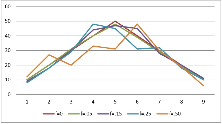
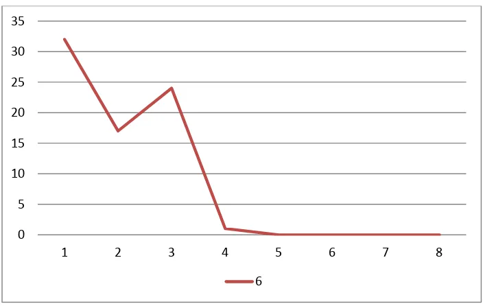
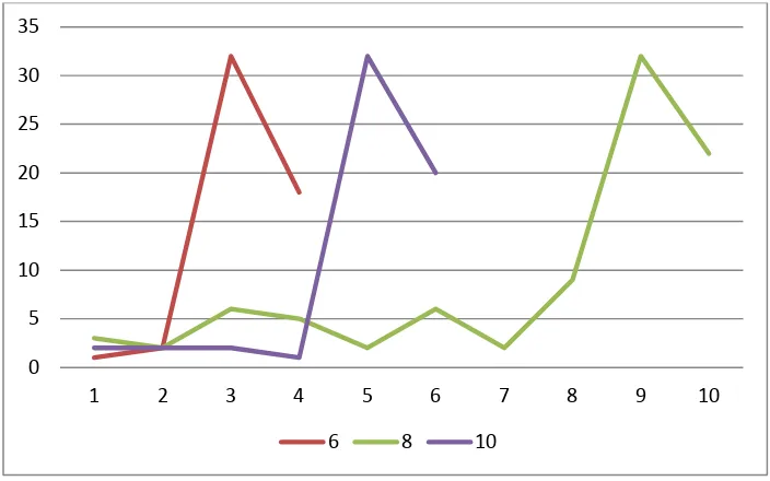
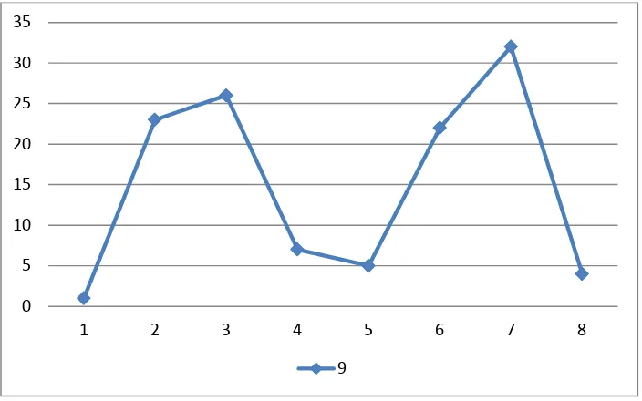
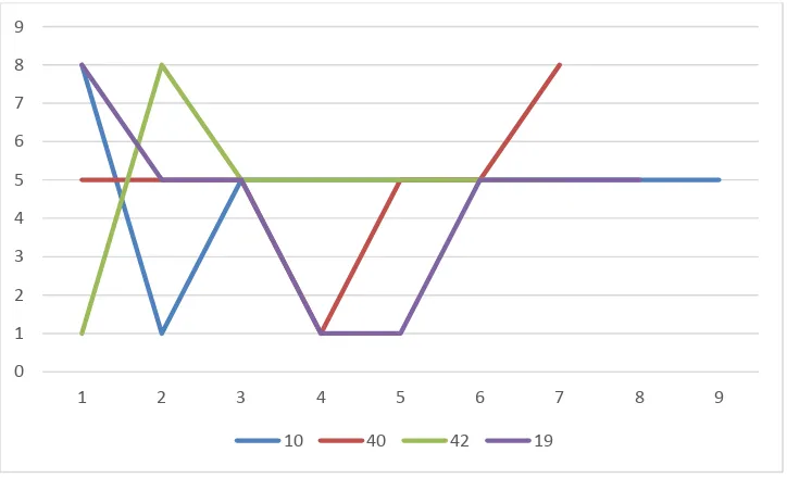
Thirty five time series representing weekly sales units of products have been created. Each of these time series have a repeated yearly patterns resulting from a combination of the 5 motifs seen in the Figure 2.5 below. These patterns vary in their shape and their length. Note that some patterns such as A and B, as well as C and D are similar in shape, but the distinctness of the motifs is in their length. The breakdown of the patterns and counts of each pattern is given in Table 2.1.
Figure 2.5 - Motif centroids for the test set 0
10 20 30 40 50 60 70 80
0 2 4 6 8 10 12
Co
u
n
t
Time Point
Table 2.1 - Patterns associated with time series Pattern Number of
Series
ID Range
ACE 10 T1-T10
BDE 15 T21-T35
ABA 5 T71-T75
CDE 1 T76
BCC 1 T77
CEE 1 T78
AAE 1 T79
DEA 1 T80
For the creation of these series, an interval of weeks between each motif is placed based on the Uniform Distribution on the interval [0, p] where p is 10 for all series except for BDE where it is 11. The values of the function between motifs are a rounded average of the last value of the previous motif and the first value of the future motif. The yearly pattern created from this process and the motif pattern is then copied 4 times to create a 4 year data set. To simulate differing entry/exit times as well as differing seasonality patterns for the data, truncation to the first xi,1 weeks and the last xi,2weeks of time series Ti such that xi,1, xi,2~Uniform(0,52).