ABSTRACT
HSU, CHIN-JUNG. Data-Driven Performance Optimization in the Cloud. (Under the direction of Dr. Vincent W. Freeh.)
Cloud computing, specifically the infrastructure-as-a-service (IaaS), allows one to lease and manage computing infrastructure and shifts costs from capital expenditure to operational expense—the pay-as-you-go model. Therefore, cloud computing shifts the paradigm of hosting infrastructures because users now can choose resource configurations that fit their performance and cost requirements. Consequently, instead of tuning workloads for the architecture they own, users now tune the architecture for the application and workload.
Cloud architecture tuning (CAT) finds the “right” resource configurations. CAT is a critical task because poor choices may lead to more than 20 times slowdown or 10 times overrun. However, this architecture tuning can be a daunting task for users. First, the search space (of architectural choices) is large and therefore, na¨ıve methods, such as brute force and random sampling, are either too expensive or too unreliable to consider. Second, workloads perform very differently on distinct architecture configurations. Guaranteeing near-optimal solutions is hard. Third, users run arbitrary workloads on diverse systems such as Hadoop and Spark. Supporting any workload and any system becomes critical. Last, users do not necessarily have the detailed knowledge about their workloads and systems. Users cannot fully benefit from cloud computing unless we can solve these challenges and make CAT widely accessible.
In this dissertation, we design and implement an efficient,effective, andreliable CAT system that delivers near-optimal solutions in anautomatic andscalable way. Our CAT system involves three essential elements, extracting low-level insights—better characterizing workloads and predicting system performance, building accurate performance models—efficiently searching the architectural space, andoptimizing tuning process—reliably converging to the near-optimal choices.
First, we propose using low-level system metrics to extract performance insights—such as CPU usage, memory pressure, and working size—that characterize workloads and identify performance bottleneck. We use lightweight monitoring tools to collect system-level metrics from each machine of a distributed system. Our method supports workloads and systems running at any sizes. The extracted insights help capture behavior of distributed storage and big data analytics systems, and decide, for example, the proper virtual machine types.
©Copyright 2018 by Chin-Jung Hsu
Data-Driven Performance Optimization in the Cloud
by Chin-Jung Hsu
A dissertation submitted to the Graduate Faculty of North Carolina State University
in partial fulfillment of the requirements for the Degree of
Doctor of Philosophy
Computer Science
Raleigh, North Carolina
2018
APPROVED BY:
Dr. Xipeng Shen Dr. Hung-Wei Tseng
Dr. Guoliang Jin Dr. Vincent W. Freeh
DEDICATION
To my parents for their endless support and love, and
to the little boy,
who had fallen so many times and still marches forward, for his na¨ıve courage and strive
BIOGRAPHY
ACKNOWLEDGEMENTS
I would like to thank many people for their support, discussion, and company in many ways and many aspects. Without them, I could not make possible this dissertation.
First and foremost, I would like to thank my advisor Dr. Vincent Freeh for his guidance, openness, and inspiration. With his encouragement, I was able to find a way out in the darkness during research. With his insight, I was able to enjoy the most precious piece of research that greatly broadens my views on a problem. And yet with numerous discussions with him, I was able to approach research problems gradually and shape this dissertation.
I would then like to thank my dissertation committee members, Dr. Hung-Wei Tseng and Dr. Xipeng Shen and Dr. Guoliang Jin, for their valuable feedback and insight on my dissertation. I would like to specially thank Dr. Hung-Wei Tseng for his advice and moral support.
I want to thank NetApp for providing me the opportunity of exploring new problems and for extending my research to machine learning. I would like to thank my mentor, Steven Yep, who led me into data-driven approaches.
I would also like to thank AT&T Labs Research, where I published my first-author paper during my PhD program. I have learned so much and built my confidence from the collaboration with Dr. Rajesh Panta and Dr. Moo-Ryong Ra.
I would like to thank other current and former PhD students, Anson Ho, Dr. Heip Nguyen, Dr. Daniel Dean, Dr. Kamal Kc and Vivek Nair, for their friendship, discussion, feedback and support. In particular, I would like to thank Vivek and Karen for their times and efforts to fight for several paper submissions together.
I want to thank Dr. Wu-Chun Chung, who brought me to the voyage of research. Without his encouragement, I would not be able to walk this far.
I also have to thank several friends I met in Raleigh. Without your taking care of me, I would not be able to move on for those ups and downs in life.
TABLE OF CONTENTS
LIST OF TABLES . . . .viii
LIST OF FIGURES . . . ix
Chapter 1 Introduction . . . 1
1.1 Summary of the State of the Art . . . 2
1.2 Thesis Statement . . . 3
1.3 Research Challenges . . . 3
1.4 Contributions . . . 4
Chapter 2 Background and Related Work . . . 6
2.1 Data-Intensive Computing . . . 6
2.2 Storage Architecture for Data-Intensive Computing . . . 9
2.3 Performance Prediction and Optimization . . . 11
2.3.1 Workload Characterization . . . 11
2.3.2 Machine Learning . . . 11
2.3.3 Low-Level Insights . . . 12
2.3.4 Sequential Model-based Bayesian Optimization . . . 12
2.3.5 Bayesian Optimization . . . 13
2.3.6 Hyper-Parameter Tuning . . . 14
Chapter 3 End-to-End Performance Prediction for Cloud Storage . . . 16
3.1 Introduction . . . 16
3.2 Mapping from Low to High . . . 18
3.2.1 Important Considerations . . . 18
3.2.2 Feature Selection . . . 19
3.2.3 A Two-Level Approach . . . 21
3.3 The Inside-Out Design . . . 21
3.3.1 Collecting and Pre-Processing Low-Level Metrics . . . 21
3.3.2 Exploring Learning Methods . . . 23
3.3.3 Two-level Training . . . 24
3.4 Evaluation . . . 24
3.4.1 Setup . . . 24
3.4.2 The Comparison Method . . . 25
3.4.3 Baseline: Prediction Performance on Static Deployment . . . 27
3.4.4 Prediction Performance in a Multi-tenant Cloud . . . 31
3.4.5 Online Self-Learning . . . 34
3.4.6 Discussion . . . 34
3.5 Conclusion . . . 35
Chapter 4 Cloud Architecture Tuning . . . 36
4.3 Challenges . . . 37
4.4 State-of-the-Art Approaches . . . 42
4.5 Problem Formalization . . . 43
4.6 Time-Cost Trade-Offs . . . 45
4.7 Conclusion . . . 47
Chapter 5 Low-Level Augmented Bayesian Optimization. . . 49
5.1 Introduction . . . 49
5.2 The Fragility Issue . . . 52
5.3 Approach . . . 54
5.4 Evaluation . . . 57
5.4.1 Experimental Method . . . 57
5.4.2 Comparison . . . 58
5.5 Discussion . . . 60
5.5.1 Bayesian Optimization in Practice . . . 60
5.5.2 Time-Cost Trade-off . . . 62
5.6 Hybrid Bayesian Optimization . . . 64
5.7 Conclusion . . . 66
Chapter 6 Scout: System Design and Implementation . . . 67
6.1 Introduction . . . 67
6.2 Design Choices . . . 68
6.3 From Observation to Action . . . 70
6.3.1 Exploration vs. Exploitation . . . 70
6.3.2 Core Techniques . . . 71
6.3.3 Search Hints . . . 73
6.3.4 Search Strategy . . . 74
6.3.5 Putting It All Together . . . 74
6.4 Implementation . . . 75
6.5 Evaluation . . . 76
6.5.1 Experiment Setup . . . 76
6.5.2 Comparison Method . . . 77
6.5.3 Is Scout effective and efficient? . . . 79
6.5.4 IsScout reliable? . . . 82
6.5.5 WhyScoutworks better? . . . 83
6.5.6 Example Search Process . . . 84
6.6 Discussion . . . 87
6.7 Conclusion . . . 89
Chapter 7 A Collective CAT Optimizer for Multiple Workloads . . . 90
7.1 Introduction . . . 90
7.2 Why Collective Optimization . . . 92
7.3 Finding the Exemplar Cloud Configuration . . . 93
7.3.1 Empirical Study . . . 93
7.3.3 Problem Formulation . . . 97
7.3.4 The Multi-Armed Bandit Problem . . . 97
7.3.5 Heuristics . . . 98
7.4 Evaluation . . . 100
7.4.1 Comparison Method . . . 100
7.4.2 Experiment Setup . . . 100
7.4.3 CanMicky identify the exemplar cloud configurations? . . . 101
7.4.4 When not to useMicky? . . . 102
7.4.5 Why UCB is the preferred choice? . . . 103
7.5 To Eliminate Sub-Optimal Choices . . . 104
7.6 Conclusion . . . 105
Chapter 8 Workload-Aware Data Placement . . . .107
8.1 Introduction . . . 107
8.2 Modeling Data Replication and Placement . . . 109
8.3 Workloads . . . 111
8.3.1 Workload Characteristics . . . 114
8.3.2 Data Placement Steps . . . 117
8.3.3 Tradeoffs in Placement Strategy . . . 119
8.4 Evaluation . . . 121
8.4.1 Experiment Setup . . . 121
8.4.2 Workload Generator and Benchmark Suite . . . 122
8.4.3 Benchmark Steps . . . 122
8.4.4 Steady-State Throughput . . . 123
8.4.5 Robustness Comparison . . . 126
8.4.6 Micro Benchmark . . . 126
8.4.7 Summary . . . 128
8.5 Conclusion . . . 128
Chapter 9 Conclusions and Future Work . . . .129
9.1 A Practical Guide to Cloud Optimizer . . . 129
9.2 Conclusion . . . 130
9.3 Future Work . . . 131
LIST OF TABLES
Table 3.1 Important features selected by different algorithms are not deterministic . 20 Table 3.2 Common scenarios that storage behavior can change in a software-define
storage environment . . . 26
Table 3.3 Ceph and COSBench settings for data collection. . . 27
Table 4.1 The evaluated applications. In total, there are 30 applications and 107 workloads measured on Hadoop 2.7, Spark 1.5 and Spark 2.1. . . 38
Table 4.2 Dataset description.The benchmark programs are taken from HiBench [59] andspark-perf [115]. . . 39
Table 4.3 The execution time and resource cost of applications running with different numbers of CPUs and memory per CPU. The text in bold refer to the configurations on the convex hull in Figure 4.5. . . 46
Table 7.1 Normalized performance on a selected group of VM types and workloads. The number 1.0 represents the optimal choice across the 18 VM types for the particular workload. . . 96
Table 7.2 The most cost-effective VM types for 107 workloads recommended by Micky The number above each column label represents normalized performance (to the optimal). CherryPick finds good (<1.2) VM types in 86% of workloads. . . 102
Table 7.3 The knee point when Micky should not be used. The knee point (the number of recurrence of workloads) represents a trade-off between search performance and measurement cost. . . 103
Table 8.1 Load-imbalance of workloads. . . 117
Table 8.2 Steady-State Throughput Comparison (instance storage) . . . 123
Table 8.3 Steady-State Throughput Comparison (NFS) . . . 125
Table 8.4 Normalized System Statistics of Roxie Servers . . . 127
LIST OF FIGURES
Figure 2.1 A MapReduce job consists of the map, shuffling and reduce phase. The map task processes a portion of input data and the reduce task aggregate the output from map tasks. The phase between the map and the reduce phase to dispatch intermediate result is the shuffling phase. . . 7 Figure 2.2 System configuration of Hadoop. Each slot handles one input split and
uses the RecordReader object to read data from a POSIX compliant file system or a non-POSIX compliant file system, e.g. distributed data store. 9
Figure 3.1 Four statistical features used in Inside-Out to capture load and internal status of a distributed storage system. The numbers and metrics represent low-level performance data collected from storage nodes. . . 19 Figure 3.2 Prediction accuracy is inconsistent due to the large feature space. Learning
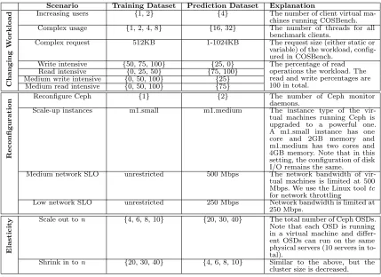
methods fail to select the right features in some cases. Dimension reduction (PCA with 10 components) does not help in this case. In the trial-and-error case, we select a subset of metrics, e.g.mean(disk.read),sum(network.recv) and std(cpu.usr). . . 21 Figure 3.3 Analysis of performance models with diverse workloads. Each bar is the
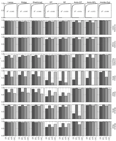
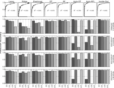
average prediction accuracy. The top row is the probability density function of prediction accuracy for each performance model. . . 28 Figure 3.4 Comparison of performance models when the storage service is reconfigured:
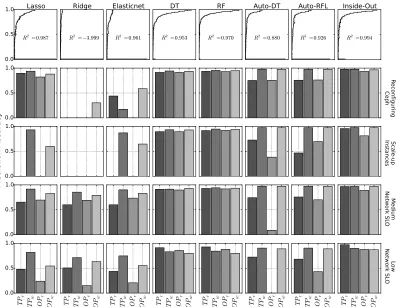
Ceph, VMs and network SLOs . . . 30 Figure 3.5 Comparison of model performance in the on-demand scaling scenario. In
the scale-out scenario, a performance model trained with 10 Ceph nodes is used to predict the performance of Ceph cluster with 20, 30 and 40 nodes. 32 Figure 3.6 Prediction accuracy in a multi-tenancy scenario. Tenant A-1 is co-located
with Tenant B-2. Tenant A-1 is throttled at 250Mbps. Tenant B-1 and B-2 are co-located without any traffic throttling. . . 33 Figure 3.7 Application of Inside-Out to real time prediction of read throughput on a
10-node Ceph cluster. Inside-Out starts from a simple prediction model trained by our collected benchmarking data. Inside-Out keeps learning the storage behavior while improving prediction accuracy over time. . . . 33 Figure 3.8 Kernel density function of prediction accuracy from Figure 3.3 to Figure 3.6.
Each colored line represents the density function of a modeling approach. Inside-Out is more consistent and accurate across almost every prediction case. . . 35
Figure 4.2 Performance distribution over different workloads. The performance is normalized to the optimal performance measured in the 18 virtual machines. Thex-axis represents workloads, sorted by their normalized performance. Both choosing the most expensive and the cheapest VM types are not desirable. . . 40 Figure 4.3 Running application with different input sizes result in very different
performance. The best performing VM types for an application can change when the input size or parameters are changed. . . 41 Figure 4.4 The performance of running the regressionworkload on instances with
different VM types. Introducing cost creates a level playing filed, in which several inferior VM types in execution time are now competitive in deployment cost. This observation implies that searching for the most cost-effective configuration is harder than searching for the fastest configuration. 42 Figure 4.5 Applications’ execution time and resource costs with different configurations. 47 Figure 4.6 The speedup and cost saving by CPU scaling (1GB memory per CPU). . 48
Figure 5.1 The number of measurements required by Bayesian Optimization (as used in [3]) to find the optimal VM type. We observe that 50% and 85% of the workloads (shown in dashed lines) require 6 (33% of the search space) and 12 (66% of the search space) measurements respectively. Bayesian Optimization is not always effective for any workload. The fragility problem—either incurs high search cost or yields sub-optimal solution (as in Region II and Region III). . . 50 Figure 5.2 Using Bayesian Optimization to find the best VM type for running the ALS
algorithm on Spark. The horizontal axis represents the search cost, and the vertical axis represents the execution time of the workload (for both lower is better). The edges of the colored area represents the 25 and the 75 percentile of the execution time. A naive Bayesian Optimization method progresses slowly towards the optimal VM type. The low-level augmented BO method alleviates the fragility problem as shown in Figure 5.6a. . . . 51 Figure 5.3 The number of actual measurements required to find the optimal VM
type by Bayesian Optimization with different kernel functions. Each kernel function is tested with 100 different sets of initial points uniformly selected. The points represent the median performance from 100 runs. . . 52 Figure 5.4 A memory bottleneck is identified by low-level performance information.
Figure 5.5 Search cost of finding the optimal VM type across the 107 workloads. The y-axis represents the cumulative percentages of workloads. In Region I, although Augmented BO does not find the optimal VM type at the fourth step, it does find a very near optimal solution with only 4% difference. Section 5.5 provides further details. . . 58 Figure 5.6 Examples of searching for the best VM. The objective is to find the
fastest VM in subfigures (a, b) and the most cost-effective VM in subfigure (c). Both the BO methods stops after they find the optimal VM type (normalized to 1.0). The line represents the median value of the execution time over 100 repeats. Each repeat used different initial points to seed BO. The shaded region represents the IQR or Interquartile range is the difference between 3rd and 1st quartile. A high value (larger area) of IQR indicates high variance. . . 61 Figure 5.7 Comparison between effectiveness of search with different stopping criteria.
There is a trade-off between search cost and deployment cost. In Region I, Augmented BO is comparable with Naive BO in terms of deployment cost but can greatly reduce search cost at the expense of slight increase in deploymwnr cost. ForRegion II andRegion III, Augmented BO outperform Naive BO for both search cost and deployment cost. . . 63 Figure 5.8 Overall comparison for the two BO methods in finding the most
cost-effective VM type across the evaluated 107 workloads. The numbers are calculated as the reduction percentage in search cost and improvement in deployment cost, both higher the better. Workloads in (0,0) represent workload which achieve similar performance in both methods. . . 64 Figure 5.9 Similar to Figure 5.8, the optimization objective is to find the best
config-uration both in execution time and search cost. Augmented BO supports finding the best VM type, given a time-cost tradeoff. . . 65
Figure 6.1 An overall comparison with other CAT methods.A search-based method better tolerates prediction bias. Relative ordering better captures the workload-architecture-performance relationship. Leveraging low-level metrics improves search performance. Historical data helps eliminate unnecessary exploration overhead in a search. Transfer learning greatly reduces search cost. . . 69 Figure 6.2 On the model selection of predicting the next step. We evaluate
the ability to distinguish a good and a bad configuration. In regression, we test rank preserving as prediction accuracy [87]. . . 73 Figure 6.3 Scout’s implementation. . . 75
Figure 6.4 Minimizing Execution Time. The x-axis represents the normalized perfor-mance (to the optimal configuration), and the optimal perforperfor-mance is 1. Scout finds the near-optimal solutions (<1.1) in 87% workloads while using much fewer steps. . . 77 Figure 6.5 Minimizing Running Cost. Searching for the optimal cost is more difficult
because the search cost is higher than the scenario of minimizing execution time.
Figure 6.6 Quality of found solutions.Although both CherryPick andScoutfind the near optimal-solutions in most of the time, Scoutis less fragile. . . 79 Figure 6.7 Stopping awareness. Search optimization avoids unnecessary search cost if it
knows when the optimal solution is found. . . 80 Figure 6.8 Convergence speed.Scoutfinds a better solution with 25% improvement (on
average) at each iteration, which suggests Scoutis more likely to converge. . . 80 Figure 6.9 Finding the fastest configuration for PageRank on Hadoop.Left & right
sub-figure show the search path of CherryPick andScoutrespectively.Scout identifies PageRank as a compute-intensive workload. It chooses the configurations with higher core counts and CPU speed. . . 82 Figure 6.10 Minimizing the running cost for Naive-Bayes on Spark.This is a
memory-intensive workload.Scoutdoes not even try thec4family due to its small memory per core. . . 84 Figure 6.11 Minimizing execution time of Regression on Spark.Since the Regression
workload requires both computation and large memory,Scoutdirectly chooses configurations with the r4 family and larger cores. . . 85 Figure 6.12 Finding the cheapest configuration for Terasort on Hadoop.The
Tera-sort workload requires enough memory to avoid spilling data to disks. Besides, a large cluster can be insufficient due to the shuffle phase in MapReduce. Scout chooses a smaller cluster with the general-purpose VM type. . . 86 Figure 6.13 Tuning the probability threshold. A smaller threshold generates a longer
search path but ensures better search performance. . . 87 Figure 6.14 Tuning the misprediction tolerance. A higher tolerance to mispredictions
generates higher search cost. . . 88 Figure 6.15 Universal performance models. Training data form multiple systems
improves prediction. . . 89
Figure 7.1 Opportunity to find the exemplar VM instances across work-loads for reducing operational cost. The y-axis represents the per-centage of workloads (out of 107 in three systems) that are within 30% difference with the optimal performance. The colored bars are VM types that considered the exemplar configurations for the majority of workloads (>= 50%). Theredbar represents that the VM type is more likely to be the optimal choice. . . 94 Figure 7.2 Search performance of optimization methods in search for cost-effective
cloud configurations.Three software systems are evaluated.CherryPick finds good solutions in the three systems while Micky is comparable in Hadoop 2.7 but shows higher variance (sub-optimal choices). We propose a integrated system (in Figure 7.5) to detect those sub-optimal cases for improvingMicky.. . . 99 Figure 7.3 Low measurement cost in collective optimization. CherryPick
op-timizes each workload separately while Micky finds the exemplar cloud configuration suitable for a group of workloads. . . 102 Figure 7.4 Selection of multi-armed bandit algorithms.The parameter (in the
Figure 7.5 A system integration to alleviate sub-optimal choices in some workloads. Scout answers “is there a better configuration than the current choice?” [62]. An integration of Micky andScoutdelivers a more efficient and reliable recommendation system of cloud configurations. . . . 104 Figure 7.6 Detection of mis-predictions usingScout.The percentage represents
the truth positive ratio, the probability the unsettled configurations can be identified. The two optimization objectives are to find the fast configuration and the most cost-effective VM type respectively. . . 105
Figure 8.1 Uniform data placement is suboptimal. The lower bar is the measured throughput of uniform placement while the upper bar is the performance loss to the idealistic placement. (Data is a subset of data shown in Table 8.2 on Section 8.4.) . . . 108 Figure 8.2 The workload demand exceeds the system capacity. . . 112 Figure 8.3 Different data placement schemes. . . 113 Figure 8.4 The load distribution among nodes under the coarse-grain data placement
(M = 64, k= 1). . . 115 Figure 8.5 The load distribution among nodes under the fine-grain data placement
with variousk (M = 64, R= 2). . . 116 Figure 8.6 The number of unique partitions per node (storage footprint) under
different placement schemes. . . 120 Figure 8.7 The number of unique partitions per node under the compact method
with variousk. The number converges at k= 32, which is equal to 1/R. . 121 Figure 8.8 Compare robustness under slight workload mispredictions. The y-axis
Chapter 1
Introduction
Cloud computing presents a paradigm shift of hosting applications [11]. Cloud computing, specifically the infrastructure-as-a-service (IaaS), allows one to lease and manage computing infrastructure and shifts costs from capital expenditure to operational expense—the pay-as-you-go model. This model is highly preferable to dynamic workload because applications can be appropriately sized—users pay only what they need. Moreover, IaaS supports a wide range of resource configurations. Users now are given the flexibility to determine the amount and type of resources for a workload at a time in order to meet desired performance and cost objectives.
Such flexibility enables new possibilities of hosting applications in the cloud—instead of tuning a workload for architecture, users tune architecture for a given workload. Performance and cost are two primary objectives in tuning. When performance is the primary concern, we can choose to, for example, increase provisioned resources to handle the growth of workload demand. On the other hand, we can tolerate slower execution in low-priority jobs for reducing running cost. In practice, there is always a trade-off between performance and cost—neither the fastest nor the cheapest is truly desired.
IaaS is promising, but much work awaits us for releasing its potential. Hosting an application in the cloud requires choosing the “right” architectural configurations that meet desired performance and cost objectives. Poor choices may lead to more than 20 times slowdown in execution time or 10 times increase in running cost [63]. Na¨ıve approaches such as brute force and random sampling are either too expensive (in evaluation) or too unreliable (in outcome) to consider. Therefore, it is a challenging task to decide the best architectural configurations in the cloud.
large search space.
Second, finding the optimal choice is time consuming and can be very expensive because characterizing workloads and predicting system performance requires an understanding of application behavior and system design. Workloads can perform very differently against distinct architecture configurations. Exhaustive search is not considered practical. Furthermore, there might be multiple choices that satisfy the given objectives. We need an effective method to recommend the near-optimal solutions.
Third, users run different kinds of workloads—such as big data analytics and machine learning tasks—in IaaS. Furthermore, workloads run on different distributed systems such as Hadoop [8], Spark [9], and High-Performance Computing Cluster (HPCC) [60]. We need a reliable method that delivers efficient and effective solutions across diverse workloads and systems.
Last, users do not necessarily have the sufficient knowledge of their running workloads and deployed systems. We need atransparent method that assists users to optimize architectures.
In this dissertation, we build an efficient,effective, andreliable system that enables cloud architecture tuning (CAT) for a workload in an automatic, scalable and economical way. Our system is transparent to users and scalable to support diverse workloads and systems. We leverage low-level performance metrics to identify resource requirements for various performance better. Our approach follows Sequential Model-Based Optimization (SMBO) that converges to the near-optimal solution iteratively. More specifically, we use a variant of Bayesian Optimization, which collects performance data, builds machine-learning based prediction models and selects the architectural configurations that are likely to perform better. Our experimental results show that data-driven methods with machine learning techniques create an efficient, effective and reliable solution to the CAT problem.
1.1
Summary of the State of the Art
The CAT problem can be cast into a learning problem—which uses elaborate offline evaluation to generate a machine learning model that predicts the performance of workloads [124, 134] and anoptimization problem—which successively evaluates configurations looking for one that is near optimal [3, 63]. The state of the art techniques such as CherryPick [3] and PARIS [134] suffer from critical issues such as prediction accuracy, cold start, and fragility.
1.2
Thesis Statement
This dissertation aims to optimize system performance in an automatic, scalable and effective way. We believe that data-driven approaches are essential this goal. In this dissertation, we argue that:
Using low-level performance insights, machine learning better characterizes
workloads and predicts system performance, resulting in better tuning architecture
for a workload in the cloud.
We first demonstrate that low-level performance information is a good proxy to capture workload and system performance. We then present how to leverage level low-level performance metrics to build accurate prediction model of system performance. Last, we build a robust system that is able to effectively tune architecture for given workloads and objectives in the cloud.
1.3
Research Challenges
Building an efficient, effective and reliable CAT method in an automatic and scalable way involves overcoming the following research challenges:
• Black-box:Users run arbitrary workloads on arbitrary systems. Any CAT method should be non-intrusive and should require no expert knowledge.
• Accurate Modeling: Since the knowledge of workloads and systems is not available, characterizing workloads and predicting system performance is difficult because only partial information (such as execution time of workloads and system metrics of runtime) is available. An effective CAT method demands accurate performance models.
• Low-overhead:Predicting performance relies on online data collection. Such data col-lection (or evaluation) is expensive because it involves running the workload. This is essentially the exploration-exploitation dilemma [69]. Therefore, any CAT method should operate at low cost.
1.4
Contributions
In this dissertation, we make the following contributions.
• Extracting low-level insights:
We design a conversion method that enables extracting performance insights from low-level performance metrics (such as CPU usage, memory usage, I/O latency and throughput) collected from individual components (such as virtual machines) in a distributed system. Since cloud systems can run at any sizes (the number of VMs), it is important to prepare performance data that have the same number of variables when building prediction models. We propose using statistical features to illustrate load distribution (such as load volume and hot spots). This extraction method serves as a building block throughout our work. We have applied this technique to estimating storage performance in software-defined storage and predicting workload performance of big data analytics in Hadoop and Spark. The extracted low-level insights improve performance prediction. For example, our proposed Arrow uses low-level metrics to augment Bayesian Optimization in finding the best virtual machine type [63].
• Building prediction models:
We evaluate various machine learning techniques and enhance model building process. Although machine learning tools are widely accessible, it can be difficult to derive robust prediction models due to the generalization error. Inside-Out uses a two-level learning method that combines two machine learning models to automatically filter irrelevant fea-tures, boost prediction accuracy and yield consistent prediction [61]. With low-level insights, our prediction model better characterizes workloads and captures system performance.
• Optimizing tuning process:
We propose a novel sequential model-based optimization (SMBO) method that incorporates guided search, relative ordering, low-level metrics, historical data and transfer learning. We design and implement Scoutto enable tuning architecture for any workloads and any systems.
• Optimizing data placement:
Computing Cluster). We are able to achieve 76% and 31% improvement for system throughput and query latency respectively. Furthermore, our approach exhibits better robustness to tolerate slightly mispredicted workloads to some degree.
Chapter 2
Background and Related Work
This chapter describes the necessary background that is related to the research problems addressed in this dissertation. We first describe data-intensive computing and its storage architecture. Next we discuss performance prediction for distributed systems. Last, we discuss related work that uses the data-driven approach to optimize system performance.
2.1
Data-Intensive Computing
Data-intensive computing is a class of parallel computing that processes large volumes of data and incurs significant processing time on I/O. Data-intensive computing is extremely important because of the desire to extract information from data [58, 75]. It is critical to design robust and efficient distributed systems for running applications that require significant computation and massive storage. Many systems such as Hadoop, Spark, and HPCC store and process large-scale data [8, 9, 60]. There is also a large body of work in optimizing data-intensive systems [5, 33, 42, 79, 103]. As more and more data-intensive computing is moving to the cloud, supporting data-intensive computing in cloud has emerged as a critical task.
This section describes two popular execution models, MapReduce and Dataflow, in data-intensive computing. We also describeApache Hadoop,Apache Spark, andHPCC, which are the widely deployed systems for data-intensive computing.
MapReduce Programming Model
computation [8, 37]. Applications that exploit the MapReduce model are highly scalable because it requires only loose synchronization [108]
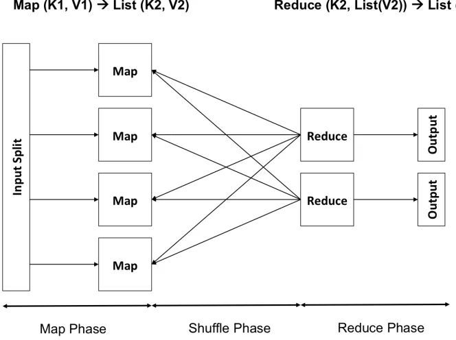
Figure 2.1 illustrates the three phases in a MapReduce job. First, the map phase processes a portion of input data, e.g., one line of a file or a XML document, and generates a list of key-value pairs. Second, the shuffle phase aggregates multiple lists of key-value pairs, and groups them by the key. The results are then redistributed to corresponding reduce tasks. Finally, the reduce phase processes the aggregated output.
Figure 2.1 A MapReduce job consists of the map, shuffling and reduce phase. The map task processes a portion of input data and the reduce task aggregate the output from map tasks. The phase between the map and the reduce phase to dispatch intermediate result is the shuffling phase.
Dataflow Execution Model
There are several variants of the dataflow model. Dryad is a general-purpose distributed execution engine that supports of coarse-grain data parallelism [65]. Vertexes are the programs and edges represent communication channels. Dryad distributes computation vertexes to a set of distributed computers. Their communication are handled by either files, TCP pipes, and shared-memory FIFOs. Other attempts include bulk synchronous parallel processing in Pregel [80] and serving trees inDremel [82].
Apache Hadoop
Apache Hadoop is an open-source implementation of the MapReduce programming model, and it is a reliable and scalable system for data processing [8]. Apache Hadoop includes four modules: 1) Hadoop YARN is a cluster resource management framework, 2) Hadoop MapReduce is the implementation to support the MapReduce programming model based on YARN, 3) Hadoop HDFS is a distributed storage system for Hadoop application data, and 4) Hadoop Common is the common utilities that are required by the above modules.
The Resource Manager (RM) is responsible for resource allocation. Once received a MapRe-duce job, RM allocates resource, e.g., CPU and memory, to initialize a AppMaster. This AppMaster is created to negotiate computing resources with the resource scheduler, e.g., FIFO Scheduler, Capacity Scheduler [26], and Fair Scheduler [43]. These schedulers allocate resources (or slots) to the AppMaster based on objectives such as data locality or fairness. Those allocated
resources can be used to run map or reduce tasks.
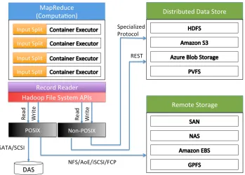
After obtaining computation resources, the AppMaster starts multiple node containers to process input splits. Each map task handles an input split, and the size is usually 64MB or 128MB (the block size of HDFS). The map task usesRecordReader andFSDataInputStreamto access input data as shown in Figure 2.2. It is possible to store data on various storage systems such as parallel file systems and object storage.
Apache Spark
Apache Spark is an in-memory data processing engine [9]. Apache Hadoop uses a linear data pipeline, which reads and writes data into disks in the map and reduce phase. This implementation does not fit well to iterative computation, which is a common requirement for applications such as in machine learning.
High-Performance Computing Cluster (HPCC)
High performance computing cluster (HPCC), also known as data analytics supercomputer, was developed by LexisNexis Risk Solutions [60]. It is a parallel system that is designed for processing large-scale data. Thor is adata refinery that processes large datasets in parallel. It is a batch processing engine that was designed for tasks similar to those that MapReduce handles best. Roxie is adata delivery engine that responds to queries. It finds the answers to requests in an index that is partitioned and, if desired, replicated across the nodes. Thor generates indexes for Roxie.
The division of labor, into data refinery and delivery engine, allows each cluster to be optimized for its task. Thor is optimized for processing large datasets in parallel where the goal is end-to-end throughput. Roxie is optimized to handle massive amounts of concurrent requests with low latency.
2.2
Storage Architecture for Data-Intensive Computing
The most common way to deploy a Hadoop system is to configure a node to run both Hadoop MapReduce and Hadoop HDFS, which can avoid bringing data to computation. However, data management, in many cases, requires separating computing and storage nodes for flexibility and efficiency. For example, enterprises prefer silos in order to manage high-value data. Amazon Elastic MapReduce primary uses Amazon S3 for its persistent data storage. Moreover, many high performance files systems are considered to replace HDFS in order to support both MapReduce application and other workload. As a result, different scenarios require different ways to deploy Hadoop. As shown in Figure 2.2, we can define three major types of Hadoop configuration as follows.
Previous work compared the performance of Hadoop integrated with different types of storage architecture [108]. The author found that in thesplit architecture, in which compute and data nodes are not co-located, Hadoop has a imbalance issue of accessing data. This can lead to poor I/O performance. In the following, we discussed the use cases that integrate Hadoop with separate storage. After that, we describe scheduling methods for Hadoop and cluster that are related to our work.
Parallel File System
Several research studies show their interests in replacing HDFS with other high performance storage systems. W. Tantisiriroj et al [120] argues that parallel file systems can support diverse workloads and provides a better tradeoff between performance and reliability. The authors proposed a PVFS shim layer to incorporate data layout of PVFS to achieve data locality. Maltzahn et al. considered Ceph as a scalable alternative to HDFS [81]. The authors create a mapping layer which is similar to the PVFS one. GPFS is a shared-disked file system developed by IBM, and widely adopted in supercomputers. R. Ananthanarayananet al. from IBM Research modify data layout in GPFS, and expose this information to Hadoop [6]. These are the attempts to replace HDFS.
Enterprise Storage
Cloud Storage
Cloud storage typically refers to object storage hosted in cloud. Amazon S3 and Azure Blob Storage are two examples. Object storage manages data as objects. Different from POSIX-compatible file systems, RESTful API is a common way to access object storage. Object storage is the primary data repository on the cloud. Many data-intensive systems,e.g., Amazon Elastic MapReduce and Azure HDInsight, support using object storage as the back-end storage [4, 133]. It is generally considered suboptimal than the Hadoop reference architecture [8].
2.3
Performance Prediction and Optimization
In this section, we describe the techniques to capture workloads and predict workload and system performance. We also discuss using data-driven approach to optimizing performance.
2.3.1 Workload Characterization
Storage performance modeling has been extensively explored in prior work. Three common modeling techniques are analytical, simulation, and data-driven approaches [10, 70, 111]. The analytical model requires domain knowledge to manually identify the factors that affect perfor-mance[70, 111]. Kelly et al. use a probability model to predict response time for an enterprise storage array. Ruemmler et al. found that a disk is too complex to model with analytical methods and designed a disk simulator to characterize storage behavior [105]. However, the simulation approach becomes inefficient when searching a large design space [70].
Mesnier et al. [83] propose a novel black-box approach that can describe the performance difference between two storage devices. With this approach, we can study the performance difference between two configurations and create a combined model with better prediction accuracy. Bodik et al. propose an exploration policy for quick collection of essential data required to train a performance model [18]. This policy can reduce the time required for offline and online model training. Chen et al. propose SLA decomposition that combines profiling and queuing model to derive resource thresholds for meeting application SLA [30].
2.3.2 Machine Learning
and proposes a scalable model, by combining related workload features. Noorshams et al. exten-sively analyze four different types of algorithms (including linear regression and CART models) and apply to IBM storage servers [90]. They also propose an optimization technique to search for parameters that can improve prediction accuracy. Their proposed parameter optimization complements our work for improving prediction accuracy. Machine learning has also been applied to performance modeling for virtual machines (VMs). DeepDive uses the classification technique to detect performance anomaly among VMs [91]. In [76], the authors apply regression and artificial neural network to model performance of a single VM.
2.3.3 Low-Level Insights
Low-level performance information is leveraged to identify performance bottlenecks and to predict application performance. DeepDive is designed to identify performance interference of co-existing VMs [91]. Wanget al. propose using the CART model to predict storage performance. Their approach requires workload information, which may not be practical for our problem setting. Inside-out provides reliable performance prediction of distributed storage service by using only low-level performance information [61]. The authors show that high-level performance can be accurately captured by only the low-level metrics. This accurate prediction model can be used to adjust resource allocation for meeting performance objectives.
2.3.4 Sequential Model-based Bayesian Optimization
Sequential model-based optimization (SMBO) is an optimization method that supports any black-box function [38]. SMBO is naturally applicable to finding the best VM. SMBO iteratively measures solutions (VM types) to optimize for an objective (execution time or deployment cost). A typical SMBO algorithm is described in Algorithm 1. An SMBO algorithm requires 4 inputs namely, a cloud set up to run a workload (f), list of VM characteristics (vm∈VM) or instance space, an acquisition function (S), and a choice of surrogate model (M). SMBO starts with an initial sample of VMs (chosen randomly), which are then measured (D). SMBO builds a surrogate or a machine learning model to estimate to predict workload performance. This model is constructed using VM characteristics and the measured performance. A VM is selected based on the surrogate model along with a predefined acquisition function. The selected VM (xi) is then measured (f). The VM (xi) along with performance (yi) is then added to the already measured VMs (D={(vm1, y1),(vm2, y2)}). This process terminates after a stopping criterion
Algorithm 1:Sequential Model-Based Optimization for CAT Input:f,VM,S,M
Output: Near-optimal configurations 1 D := Initial sampling (f,VM) 2 for kin|VM ∈/D|do
3 p(y|vm, D) := fit a surrogate model (M, D) 4 vmk :=argmaxvm∈VMS(vm, p(y|vm, D))
5 yk :=f(vmk) 6 D:= D∪(vmk, yk)
7 if meeting stopping criteriathen
8 break
9 end
10 end
2.3.5 Bayesian Optimization
Bayesian Optimization (BO) follows the same formalism of sequential model-based optimization (SMBO). Like SMBO, BO has two essential components namely a (probabilistic) regression model, and an acquisition function (refer to [109] for more details.) BO has been used as a drop-in replacement to standard techniques such as random search, grid search and manual tuning in numerous domains such as hyperparameter tuning and software performance optimization [38, 51, 87, 142]. To solve the CAT problem, CherryPick used BO to find the best VM for a specific workload [3].
In Bayesian Optimization, Gaussian Process is the standard probabilistic model used for building the surrogate model. Gaussian Process is a distribution over objective functions specified by a mean function and covariance function. Once a surrogate model is trained, it can be used to estimate performance (of a workload) on the unmeasured VM. The surrogate model returns distribution of the estimated performance associated with the VM (mean and variance). The next VM to measure is determined by an acquisition function. Common acquisition functions are Probability of Improvement (PI), Expected Improvement (EI), and Gaussian Process Upper Confidence Bound (GP-UCB) [109]. Recently, the entropy search methods, backed by information theory, are promising alternatives [126]. In practice, EI is effective and used in CherryPick.
a practitioner needs to choose a proper kernel function to ensure smoothness in the instance space. Such a task is challenging and can affect the performance of BO. CherryPick chooses the Mat´ern 5/2 kernel function because it does not require strong smoothness, which are the cases for many real-world applications [3, 134].
2.3.6 Hyper-Parameter Tuning
System and software performance is highly affected by configurations. StarFish is an auto-tuning system for Hadoop applications [57]. BestConfig proposes the Divide and Diverge Sampling strategy along with the Recursive Bound and Search method for turning software parameters [141]. Similar framework is also proposed to automate tuning system performance of stream-processing systems [17]. BOAT is a structured Bayesian Optimization-based framework for automatically tuning system performance [35] which leverages contextual information.
BO4CO uses Bayesian Optimization to continuously optimize system performance [67]. Similar to CherryPick, BO4CO leverages Bayesian Optimization but does not consider low-level metrics.BOAT is a structured Bayesian Optimization-based framework for automatically tuning system performance which leverages contextual information [35].BOATcombines the parametric and non-parametric model for better predicting the trend in system performance. The idea behind their work and our work is very similar: leveraging domain knowledge to enhance BO. BOAT optimizes software configurations while Arrow tunes architecture (virtual machines). Parameter tuning is critical to machine learning application [38, 51, 73, 109].
Bilalet al. propose a framework to automate tuning system performance of stream-processing systems [17]. Their modified hill-climbing search with heuristic sampling inspired by Latin Hypercube shortens the search process by two to five times. The above methods reduce the search cost by a significant degree. However, they focus on performance tuning for the same workload (or application) on the same type of machine. It is not clear how to leverage their approaches to support different machine configurations in cloud computing. We, instead, find the best machine configuration for a given workload.
Sampling techniques focus on reducing sampling cost while building accurate models to optimize software systems [87, 92]. The above methods reduce the search cost by a significant degree. However, they focus on performance tuning for the same workload (or application) on the same type of machine. It is not clear how to leverage their approaches to support different machine configurations in cloud computing. We, instead, find the best machine configuration for a given workload.
Chapter 3
End-to-End Performance Prediction
for Cloud Storage
This chapter presents an approach to estimating end-to-end performance of distributed storage systems. We explain why low-level performance metrics are a desirable proxy for estimating end-to-end performance. We then present our automatic model building tool for generating robust and accurate performance models.
3.1
Introduction
Many storage systems are moving away from dedicated appliance-based storage model to software-defined storage (SDS), which separates software that provisions and manages storage from the hardware that provides raw physical storage [66, 114, 121]. This trend is partly driven by the tremendous growth of data and the emergence of cloud applications that operate in a multi-tenant environment with diverse workload characteristics. As a result, the rigid appliance-based model, with tightly-coupled hardware and software features, is no longer cost-effective, lacks flexibility, and does not scale well. SDS systems are increasingly abandoning centralized storage services in favor of distributed systems like Ceph [27], HDFS [8], Swift [94]. Distributed storage systems are attractive because they scale well, allowing storage services to grow or shrink, based on storage demands. They are also better suited to handle diverse multi-tenant workloads.
Diverse and time-varying storage workloads and performance interference in a multi-tenant environment further complicate the reliable assurance of storage QoS. Reliable and accurate monitoring of high-level storage performance metrics (e.g. throughput and IOPS) is critical for providing storage QoS guarantees. However, monitoring end-to-end storage performance is difficult in a distributed storage service. Instrumenting user applications to measure storage performance is not always practical. Performing benchmark tests in production systems also has practical limitations since they interfere with storage application workload. Furthermore, running exhaustive benchmark experiments to cover diverse application workloads, deployment topologies, and large configuration parameter space is time-consuming and impractical in many cases. Building accurate analytical performance models, on the other hand, is also difficult for the reasons mentioned above.
This chapter proposes the idea of using low-level system metrics (e.g., CPU usage, RAM usage and network I/O) as a proxy for measuring high-level performance (e.g., end-to-end IOPS and throughput) of distributed storage applications. We design, implement and evaluate a practical tool, called Inside-Out, that applies machine learning techniques to the low-level metrics collected from individual components of a distributed storage system to accurately estimate high-level storage performance metrics—like throughput and IOPS—of the entire distributed storage system. We believe that a tool like Inside-Out can serve as an important component of the overall SDS architecture.
Inside-Out takes a black-box modeling approach, which does not require knowledge about distributed storage system protocol, workload characteristics, and deployment topology. Inside-Out relies upon machine learning techniques to automatically derive an accurate end-to-end performance model. We explore several well-known machine learning algorithms including linear regression, decision tree learning, and ensemble methods [90, 125], and conclude that there does not exist an one-size-fits-all algorithm that can work in all prediction cases. Hyperparameter tuning [29, 90], model selection [74] and feature selection [54, 106] all turn out to be too complicated for optimizing prediction accuracy. In contrast, Inside-Out uses a two-level learning method that automatically selects important features, boosts prediction accuracy, and achieves consistent prediction. This two-level learning method pipelines two supervised learning algorithms to eliminate irrelevant features while avoiding overfitting problems.1
Inside-Out offers several key benefits. Unlike traditional analytic performance modeling approach, Inside-Out is more generic, and therefore can be more easily applied to different storage services. Different from previous work, Inside-Out does not require information about system configuration and application workload [10, 70, 90, 105, 111, 125, 136]. Due to the self-learning property, Inside-Out improves performance prediction accuracy with more data. It
1
can also adapt to changes in the system by continuously learning the system behavior.
We evaluate Inside-Out using Ceph [27] running on an OpenStack-based SDS platform. The low-level performance metrics are collected from participant virtual machines running various components of a Ceph storage service.2 Our in-depth evaluation shows that Inside-Out generates end-to-end performance models with 91.1% prediction accuracy on average. More importantly, as discussed above, Inside-Out is generic in nature as it captures the behavior of the storage system by analyzing low-level system metrics (that are protocol and application agnostic). Furthermore, we demonstrate that Inside-Out can provide reliable hints for performance monitoring tasks even in the presence of evolving workload characteristics, changing storage configuration and interfering tenants. We also show that Inside-Out is reliable in estimating end-to-end performance even when the storage system expands or shrinks. We show that Inside-Out provides reliable performance prediction when the storage system is up to four times larger than the one used for building machine learning models during the training phase. Lastly, Inside-Out is able to learn new storage behavior over time.
3.2
Mapping from Low to High
This section discusses the guiding principles and challenges in using low-level performance metrics to build accurate end-to-end performance models for a distributed storage system.
3.2.1 Important Considerations
This section describes how we use low-level performance metrics to predict high-level system performance. We discuss how we pick the metrics and how to transform metrics to meaningful features.
General low-level metrics
Since our goal is to provide a tool for estimating the end-to-end performance of a diverse set of storage systems, the inputs to our model need to be generic in nature, i.e., they need to be independent of storage systems or the distributed protocols used by such applications. An SDS provider should be able to obtain the input metrics without instrumenting storage application or requiring domain knowledge about the storage application. Low-level system metrics (e.g. CPU utilization, memory usage, network IO, etc.) satisfy these requirements. DeepDive uses low-level metrics to identify performance anomaly for a running VM [91]. To the best of our
2Our approach is not limited to VM-based environments. It can be applied to container-based and bare-metal
Storage Node (S1) Storage Node (S2) Storage Node (S3)
MEAN= 10
STD = 8.5
5% = 80
10 Metric A 20 Metric B
10 Metric C
10 Metric D SUM = 60
Feature Transformation
11 Metric A 35 Metric B
80 Metric C 20 Metric D
9 Metric A 15 Metric B
15 Metric C 30 Metric D
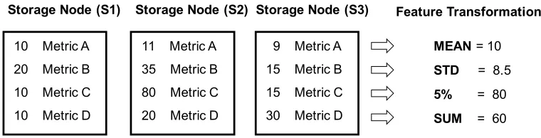
Figure 3.1 Four statistical features used in Inside-Out to capture load and internal status of a distributed storage system. The numbers and metrics represent low-level performance data collected from storage nodes.
knowledge, this work presents the first study that maps low-level system metrics to high-level end-to-end performance of a distributed storage service.
Capture important features of a distributed storage system
A distributed storage system can dynamically expand or shrink according to demand. The performance model has to capture the current scale of the deployment, the bottlenecks, and the average and variance in performance of individual components of the distributed system. For each low-level system metric collected from various components of the distributed system, we use four statistical variables to characterize the behavior of a distributed system (see Figure 3.1). The statistical variable mean andstd describe whether the impact of the workload is evenly distributed among storage components. The sum variable represents the scale of the deployment, while the variable 5% (top 5 percentile) captures the hot spot situations. The feature transformation from raw system metrics to these four statistical values also allows Inside-Out to apply the uniform input format for developing performance models for distributed systems at different scales.
3.2.2 Feature Selection
In this work, we collect low-level performance metrics from two components of Ceph namely monitor (MON) and Object Storage Daemons (OSD). We usedstat, a monitoring tool to collect resource statistics, to collect 32 low-level performance metrics in total. These measurements are then transformed using the process described in Figure 3.1 (refer to Section 3.3.1 for more details).
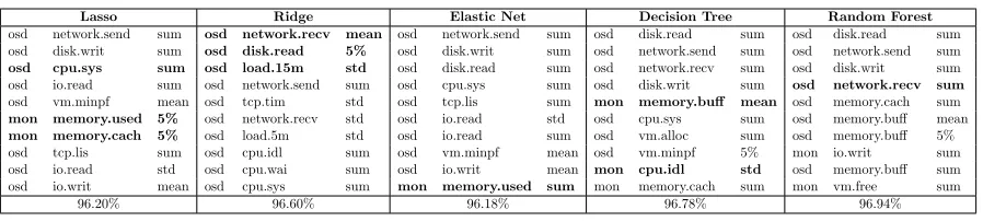
Table 3.1 Important features selected by different algorithms are not deterministic
Lasso Ridge Elastic Net Decision Tree Random Forest
osd network.send sum osd network.recv mean osd network.send sum osd disk.read sum osd disk.read sum osd disk.writ sum osd disk.read 5% osd disk.writ sum osd network.send sum osd network.send sum
osd cpu.sys sum osd load.15m std osd disk.read sum osd network.recv sum osd disk.writ sum osd io.read sum osd network.send sum osd cpu.sys sum osd disk.writ sum osd network.recv sum
osd vm.minpf mean osd tcp.tim std osd tcp.lis sum mon memory.buff mean osd memory.cach sum
mon memory.used 5% osd network.recv std osd io.read std osd cpu.sys sum osd memory.buff mean
mon memory.cach 5% osd load.5m std osd io.read sum osd vm.alloc sum osd memory.buff 5% osd tcp.lis sum osd cpu.idl sum osd vm.minpf mean osd vm.minpf 5% mon io.writ sum osd io.read std osd cpu.wai sum osd io.writ mean mon cpu.idl std osd memory.buff sum osd io.writ mean osd cpu.sys sum mon memory.used sum mon memory.cach sum mon vm.free sum
96.20% 96.60% 96.18% 96.78% 96.94%
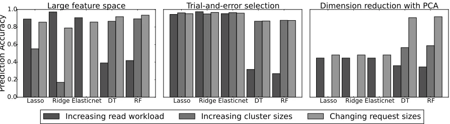
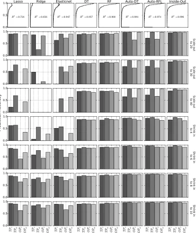
of different learning methods when modeling read throughput. We see that all learning methods achieve high model accuracy even though they choose different features. The model accuracy was obtained usingk-fold cross validation (k=10), a common technique for assessing model accuracy. The training data is partitioned intokdisjoint sets. A single data partition is used for validation purpose and the remainingk−1 partitions are used for training data. Although all models yield good model accuracy, they perform poorly and inconsistently when the storage environment changes. In Figure 3.2, we show the prediction accuracy under three types of changes in the storage environment—increase in the size of the distributed storage system, read workload and individual storage IO request size. These algorithms (discussed later in Section 3.3.2) do not yield consistent prediction accuracy any more. For example, Lasso can still predict well when workload has changed but Decision Tree cannot. On the contrary, Decision Tree performs better than Lasso when the size of the storage system increases. We suspect this is caused by the large feature space, which leads to the overfitting problem [40, 56]. Next, we manually remove most features and select only a few with a trial-and-error strategy. As shown in Figure 3.2, we see significant improvement in some cases, but not all. Since an SDS environment can change over time, it is important for our model to provide consistent prediction accuracy under system changes such as software reconfiguration and cluster expansion.
Lasso Ridge Elasticnet DT RF 0.0
0.2 0.4 0.6 0.8 1.0
Pre
dic
tio
n A
cc
ura
cy
Large feature space
Lasso Ridge Elasticnet DT RF
Trial-and-error selection
Lasso Ridge Elasticnet DT RF
Dimension reduction with PCA
Increasing read workload
Increasing cluster sizes
Changing request sizes
Figure 3.2 Prediction accuracy is inconsistent due to the large feature space. Learning methods fail to select the right features in some cases. Dimension reduction (PCA with 10 components) does not help in this case. In the trial-and-error case, we select a subset
of metrics, e.g. mean(disk.read), sum(network.recv)and std(cpu.usr).
3.2.3 A Two-Level Approach
Instead of performing feature selection or dimension reduction, we propose a generic two-step approach that can improve the consistency of prediction accuracy. In the first step, we use some heuristic methods to filter out irrelevant features. Then, in the second step, we apply machine learning algorithms to build performance models with the reduced feature set. The intuition behind this idea is that it is difficult to determine the most important performance features but it is relatively easy to eliminate unimportant features. For example, the features which are not in the top 100 list after step one can be labeled as unimportant features.
3.3
The Inside-Out Design
In this section, we present the design of Inside-Out. We also discuss the trade-offs among a set of representative machine learning algorithms and propose a two-step learning technique for mitigating overfitting problems.
3.3.1 Collecting and Pre-Processing Low-Level Metrics
3.3.1.1 Monitoring storage components
We collect low-level system metrics of the underlying operating system to capture resource utilization (e.g., cpu, memory, disk and network usage). The low-level performance metrics are sampled with one-second granularity. Such data can be collected from libvirt, Ganglia, instrumented hypervisors [21] andCeilometer in OpenStack. We usedstatmonitoring tool (with option: -tcly -mg –vm -dr -n –tcp –float) to collect these data.
3.3.1.2 Data smoothing
Building a performance model with data collected at one-second granularity is challenging because system data can exhibit high variance at small time scales, e.g., due to dynamic/bursty workloads and interference among co-located tenants. Furthermore, the storage IO operation needs to pass through a series of software layers between the storage client and the back-end raw physical storage device. The long storage IO path can introduce high variability in resource utilization at smaller time scales. For example, HDFS and Ceph both replicate data blocks across storage nodes distributed in physically disjoint servers, racks or even datacenters. To address the uncertainties due to complex IO path spanning several software layers, we compute the moving average of the collected performance data. We have empirically found that one-minute window for processing the moving average is sufficient to eliminate outliers from the raw data.
3.3.1.3 Timestamp alignment
Proper time synchronization among participating servers is essential to correlate data collected from those servers. We use NTP for time synchronization. The average timestamp of all nodes is taken as the basis for time alignment.
3.3.1.4 Feature transformation for a distributed storage system
As mentioned earlier, elasticity is an important feature of SDS, since it needs to adjust its size based on storage demand. Thus our model must accurately predict end-to-end performance at arbitrary deployment scales. However, the data collected from different scales may have different dimensions. For instance, Ceph with 10 Object Storage Servers (OSDs) generates 10 copies of low-level performance metrics, while Ceph with 5 OSDs generates fewer data points. This makes it hard to train and build a unified model. As mentioned in Section 3.2.1, we usemean, sum, std, and 5% statistical variables to capture different types of workload distribution such as hotspot,load imbalance, and aggregate performance.
stabilizing performance data. Then it calculatesmean,std,sum and5% of individual metrics collected from multiple machines. This ensures that our performance model can accept input data for systems with varying scales of deployment, while preserving important characteristics of a distributed storage system. For training and validation purposes, we measure end-to-end performance metrics (IOPS, throughput, and latency) every 5 seconds using COSbench [32], and take average over the one-minute window. Next, we describe how we build end-to-end performance models in order to capture the relationship between low-level system metrics and end-to-end throughput and IOPS.
3.3.2 Exploring Learning Methods
Our goal is to build a model that accurately predicts end-to-end throughput and IOPS by analyzing only the low-level metrics of a distributed storage system. We explore several algorithms, including statistical regression [41, 56], decision tree learning and random forests learning [56, 125]. For statistical regression, we mainly focus on linear regression techniques, which can be extended to support non-linear regression by expanding features that simulate, for example, quadratic terms [76]. We did not find this necessary in our application and exclude the discussion. Lasso is a least square linear regression technique with L1-norm regularization. The L1 penalty function leads to a sparse solution, which has an effect of restricting the number of selected variables. This property is useful for figuring out important features, especially when the number of variables or features is large.Ridge is similar to Lasso but instead uses L2-norm regularization, which has the effect of group selection of variables. This property does not restrict the number of variables selected by the prediction model and therefore, the prediction accuracy might degrade and become inconsistent when the number of input features to the training model is large. Elastic Net combines both advantages—it does group selection while enforcing sparsity. Based on our data set, Lasso and Elastic Net have similar prediction performance, and Ridge shows larger variance. TheDecision Tree (DT) learning uses a top-down approach and recursively partitions data to fit target values. The tree-based model is easy to interpret and scales well to large datasets. Random Forests (RF) is an ensemble method that uses multiple decision trees [56]. RF improves a single decision tree in many ways, e.g., accuracy, efficiency, and robustness.
Figure 3.2.
3.3.3 Two-level Training
The fundamental challenge in building an effective prediction model from a large set of features is the overfitting problem. One way to address this problem is to perform manual feature selection. However, this approach is problematic because the right set of features depend on application types, deployment topology, resource constraint, etc.
Instead, we propose a two-level training process that filters out irrelevant features in the first step and then builds models by using the reduced set of features in the second step. To this end, Inside-Out pipelines Ridge and Lasso together, where Ridge filters features in coarse-granularity and then Lasso builds the prediction model. We choose Ridge as the filtering algorithm because it is not a sparse solution and considers all features. We then apply exhaustive grid search to find the optimized score for important features. We use α×median(coefficients) derived from Ridge as the threshold.
For comparison, we consider Decision Tree with Lasso (Auto-DTL) and RandomForest with Lasso (Auto-RFL). Our evaluation shows Inside-Out outperforms consistently across all prediction cases, and boosts prediction accuracy in several scenarios, where the linear regression models fail to generalize the behavior of a distributed storage system. We also experimented by using Lasso and Elastic Net as the filter algorithm but did not find comparable performance with Inside-Out.
Inside-Out uses the following pseudo code to generate an end-to-end performance model. In practice, we setk to 10 for stable prediction results. The data processing part is explained in previous sections. Features are automatically selected using the Ridge algorithm with multiple thresholds. We vary α from 0.1,0.2, ...,1.0. The grid search approach is used to select the best model.
3.4
Evaluation
In this section, we present a comprehensive evaluation of Inside-Out. We demonstrate that Inside-Out can accurately predict end-to-end performance, i.e., throughput and IOPS, using low-level system metrics and is applicable to a wide range of realistic scenarios.
3.4.1 Setup
Algorithm 2:Inside-Out Model Building
Input: low-level performance metrics from distributed nodes Output: an end-to-end performance model
Initialisation
1: thresholds={α1, ..., αN}
2: m1 = filtering algorithm→Ridge 3: m2 = model algorithm→Lasso 4: k= k-fold cross validation
5: score= 0
Data preprocessing (refer to Section 3.3.1)
6: alignment of input data
7: calculate moving average across metrics
8: feature transformation for the distributed scenario Grid Search
9: for allt∈thresholds do
10: f eatures= executem1 with threshold t
11: score, m=max(crossvalidation(k,m2, f eatures))
12: end for
13: return m with maximum score
storage protocols, includinglibrados for Ceph, and provides a set of knobs to change storage traffic pattern. Table 3.3 lists Ceph and COSBench configurations used in our experiments.
We collected benchmarking data from an OpenStack-based SDS platform. The cluster has 16 machines, and each machine has 16 cores, 24GB memory and 250GB disk space. Each machine has 1Gbps network interface connected to a 10Gbps switch. The dataset is collected from about 5300 benchmark runs. The total dataset is composed of about 15.2 million records, each of which is a vector of 32 low-level performance data. The end-to-end performance data collected from COSBench contains 3 million records. The combined dataset is about 24GB, collected over two weeks.
3.4.2 The Comparison Method