Linear Phase FIR Digital Filter Design Using Differential Evolution Algorithms

(1)

University of Windsor University of Windsor

Scholarship at UWindsor

Electronic Theses and Dissertations Theses, Dissertations, and Major Papers

4-13-2017

Linear Phase FIR Digital Filter Design Using Differential Evolution

Algorithms

Wei Zhong

University of Windsor

Follow this and additional works at: https://scholar.uwindsor.ca/etd Recommended Citation

Recommended Citation

Zhong, Wei, "Linear Phase FIR Digital Filter Design Using Differential Evolution Algorithms" (2017). Electronic Theses and Dissertations. 5959.

https://scholar.uwindsor.ca/etd/5959

This online database contains the full-text of PhD dissertations and Masters’ theses of University of Windsor students from 1954 forward. These documents are made available for personal study and research purposes only, in accordance with the Canadian Copyright Act and the Creative Commons license—CC BY-NC-ND (Attribution, Non-Commercial, No Derivative Works). Under this license, works must always be attributed to the copyright holder (original author), cannot be used for any commercial purposes, and may not be altered. Any other use would require the permission of the copyright holder. Students may inquire about withdrawing their dissertation and/or thesis from this database. For additional inquiries, please contact the repository administrator via email

(2)

Linear Phase FIR Digital Filter Design Using Differential Evolution

Algorithms

by

Wei Zhong

A Thesis

Submitted to the Faculty of Graduate Studies

through Electrical and Computer Engineering

in Partial Fulfillment of the Requirements for

the Degree of Master of Applied Science at the

University of Windsor

Windsor, Ontario, Canada

2016

(3)

Linear Phase FIR Digital Filter Design Using Differential Evolution

Algorithms

by

Wei Zhong

APPROVED BY:

______________________________________________

Dr. Z. Kobti

School of Computer Science

______________________________________________

Dr. Huapeng Wu

Department of Electrical & Computer Engineering

______________________________________________

Dr. H. K. Kwan, Advisor

Department of Electrical and Computer Engineering

______________________________________________

(4)

iii

Declaration of Originality

I hereby certify that I am the sole author of this thesis and that no part of this thesis has

been published or submitted for publication.

I certify that, to the best of my knowledge, my thesis does not infringe upon anyone

copyright nor violate any proprietary rights and that any ideas, techniques, quotations, or

any other material from the work of other people included in my thesis, published or

otherwise, are fully acknowledged in accordance with the standard referencing practices.

Furthermore, to the extent that I have included copyrighted material that surpasses the

bounds of fair dealing within the meaning of the Canada Copyright Act, I certify that I have

obtained a written permission from the copyright owner(s) to include such material(s) in

my thesis and have included copies of such copyright clearances to my appendix.

I declare that this is a true copy of my thesis, including any final revisions, as approved by

my thesis committee and the Graduate Studies Office, and that this thesis has not been

(5)

iv

Abstract

Digital filter plays a vital part in digital signal processing field. It has been used in control

systems, aerospace, telecommunications, medical applications, speech processing and so

on. Digital filters can be divided into infinite impulse response filter (IIF) and finite impulse

response filter (FIR). The advantage of FIR is that it can be linear phase using symmetric

or anti-symmetry coefficients. Besides traditional methods like windowing function and

frequency sampling, optimization methods can be used to design FIR filters. A common

method for FIR filter design is to use the Parks-McClellan algorithm. Meanwhile,

evolutional algorithm such as Genetic Algorithm (GA), Particle Swarm Optimization (PSO)

[2], and Differential Evolution (DE) have shown successes in solving multi-parameters

optimization problems.

This thesis reports a comparison work on the use of PSO, DE, and two modified DE

algorithms from [18] and [19] for designing six types of linear phase FIR filters, consisting

of type1 lowpass, highpass, bandpass, and bandstop filters, and type2 lowpass and bandpass

filters. Although PSO has been applied in this field for some years, the results of some of

the designs, especially for high-dimensional filters, are not good enough when comparing

with those of the Parks-McClellan algorithm. DE algorithms use parallel search techniques

to explore optimal solutions in a global range. What’s more, when facing higher

dimensional filter design problems, through combining the knowledge acquired during the

searching process, the DE algorithm shows obvious advantage in both frequency response

(6)

v

Acknowledgements

I would like to express my sincere gratitude and appreciation to Dr. H. K. Kwan, who

introduced me the subject of evolutionary optimization and various optimization algorithms

for designing digital filters through an excellent set of graduate courses, assignments, and

projects, for his invaluable guidance, helps, and suggestions throughout the thesis work.

Also special thanks to Dr. Huapeng Wu and Dr. Z. Kotbi, for their expert guidance and

advices in my research. What’s more, I would also like to thank my family for their constant

(7)

vi

List of Tables

Table 2.1 Coefficients of 12th-order type1 LP-FIR filter by PSO ... 14

Table 2.2 Design result of 12th-order LP-FIR filter by PSO ... 14

Table 2. 9 Coefficients of 12th-order type1 HP-FIR filter by PSO ... 18

Table 2. 10 Design result of 12th-order HP-FIR filter by PSO ... 19

Table 2.11 Coefficients of 24th-order type1 HP-FIR filter by PSO ... 19

Table 2.12 Design result of 24th-order HP-FIR filter by PSO ... 19

Table 2.17 Coefficients of 12th-order type1 BP-FIR filter by PSO ... 22

Table 2.18 Design result of 12th-order BP-FIR filter by PSO ... 23

Table 2.25 Coefficients of 12th-order type1 BS-FIR filter by PSO ... 26

Table 2.26 Design result of 12th-order BS-FIR filter by PSO ... 27

Table 2.34 Design result of 25th-order type 2 LP-FIR filter by PSO ... 31

Table 2.36 Design result of 49th-order type 2 LP-FIR filter by PSO ... 32

Table 2.38 Design result of 25th-order type 2 BP-FIR filter by PSO ... 34

Table 2.40 Design result of 49th-order type 2 BP-FIR filter by PSO ... 35

(10)

ix

Table 3.2 Design result of 12th-order type 1 LP-FIR filter by DE ... 42

Table 3.3 Coefficients of 24th-order type1 LP-FIR filter by DE ... 42

Table 3.9 Coefficients of 12th-order type1 HP-FIR filter by DE ... 46

Table 3.10 Design result of 12th-order type 1 HP-FIR filter by DE ... 46

Table 3.17 Coefficients of 12th-order type1 BP-FIR filter by DE ... 50

Table 3.18 Design result of 12th-order type 1 BP-FIR filter by DE ... 50

Table 3.21Coefficients of 36th-order type1 BP-FIR filter by DE ... 51

Table 3.25 Coefficients of 12th-order type1 BS-FIR filter by DE ... 54

Table 3.26 Design result of 12th-order type 1 BS-FIR filter by DE ... 54

Table 4.1 Computational time of the type1 LP linear FIR filter ... 67

Table 4.2 Computational time of the type1 HP linear FIR filter ... 67

Table 4.3 Computational time of the type1 BP linear FIR filter ... 67

Table 4.4 Computational time of the type1 BS linear FIR filter ... 67

Table 4.5 Coefficients of 48th-order type1 LP-FIR filter by MPMSIDE... 73

(11)

x

Table 4.7Coefficients of 48th-order type1 BP-FIR filter by MPMSIDE ... 73

Table 4.8 Coefficients of 48th-order type1 BS-FIR filter by MPMSIDE ... 73

Table 4.9 Coefficients of 49th-order type2 LP-FIR filter by MPMSIDE... 74

Table 4.10 Coefficients of 49th-order type2 BP-FIR filter by MPMSIDE ... 74

Table 4.11 The comparison of MPMSIDE and the original DE algorithm ... 77

Table 5.1 Simulation Results for PSO, PM, and DE ... 81

(12)

xi

List of Figures

Fig. 1.1 Ideal lowpass linear phase FIR filter ... 5

Fig. 1.2 Actual lowpass FIR filter ... 5

Fig. 1.3 Linear phase FIR filter coefficients initializing method. ... 8

Fig. 2.1 Flow chart of the PSO algorithm ... 11

Fig. 2.2 Magnitude, ripple errors of 12th-order LP-FIR filter by PSO ... 15

Fig. 2.6 Convergence behaviors of PSO in design LP-FIR with orders of 12th, 24th, 36th, and 48th ... 18

Fig. 2.7 Magnitude, ripple errors of 12th HP-FIR lowpass filter by PSO ... 19

Fig. 2.8 Magnitude, ripple errors of 24th-order HP-FIR filter by PSO ... 20

Fig. 2.11 Convergence behaviors of PSO in design HP-FIR with orders of 12th, 24th, 36th, and 48th ... 22

Fig. 2.12 Magnitude, passband and stopband errors of 12th-order BP-FIR lowpass filter ... 23

Fig. 2.13 Magnitude, ripple errors of 24th-order BP-FIR filter by PSO ... 24

Fig. 2.16 Convergence behaviors of PSO in design BP-FIR with orders of 12th, 24th, 36th, and 48th ... 26

Fig. 2.17 Magnitude, ripple errors of 12th-order BS-FIR filter by PSO ... 27

Fig. 2.21 Convergence behaviors of PSO in design BS-FIR with orders of 12th, 24th, 36th, and 48th ... 30

Fig. 2.22 Magnitude, ripple errors of 25th-order type2 LP-FIR filter by PSO ... 32

Fig. 2.23 Magnitude, ripple errors of 49th-order type2 LP-FIR filter by PSO ... 33

Fig. 2.24 Magnitude, ripple errors of 25th-order type2 BP-FIR filter by PSO ... 34

Fig. 2.25 Magnitude, ripple errors of 49th-order type2 BP-FIR filter by PSO ... 35

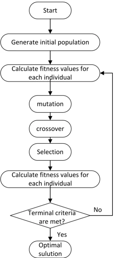
Fig. 3.1 The flow chart of DE algorithm ... 38

Fig. 3.2 Magnitude, passband and stopband errors of 12th-order LP-FIR filter ... 42

Fig. 3.3 Magnitude, passband and stopband errors of 24th-order LP-FIR filter ... 43

Fig. 3.4 Magnitude, passband and stopband errors of 36th-order LP-FIR filter by DE ... 44

Fig. 3.5 Magnitude, passband and stopband errors of 48th-order LP-FIR filter by DE ... 45

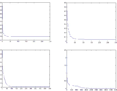
Fig. 3.6 Convergence behaviors of DE in design LP-FIR with orders of 12th, 24th, 36th, and 48th ... 45

Fig. 3.7 Magnitude, passband and stopband errors of 12th-order HP-FIR filter by DE ... 46

(13)

xii

Fig. 3.11 Convergence behaviors of DE in design HP-FIR with orders of 12th, 24th, 36th, and 48th ... 49

Fig. 3.12 Magnitude, passband and stopband errors of 12th-order BP-FIR filter by DE ... 50

Fig. 3.16 Convergence behaviors of DE in design BP-FIR with orders of 12th, 24th, 36th, and 48th ... 53

Fig. 3.17 Magnitude, passband and stopband errors of 12th-order BS-FIR filter by DE ... 54

Fig. 3.21 Convergence behaviors of DE in design BS-FIR with orders of 12th, 24th, 36th, and 48th ... 57

Fig. 3.22 Magnitude, ripple errors of 25th-order type2 LP-FIR filter by DE ... 59

Fig. 3.23 Magnitude, ripple errors of 49th-order type2 LP-FIR filter by DE ... 60

Fig. 3.24 Magnitude, ripple errors of 25th-order type2 BP-FIR filter by DE ... 61

Fig. 3.25 Magnitude, ripple errors of 49th-order type2 BP-FIR filter by DE ... 62

Fig. 4.1 The flow chart of modified DE algorithm ... 65

Fig. 4.2 Convergence speed using Shamekhi’s DE algorithm and original DE algorithm when designing type 1 Lowpass FIR filter of order 12, 24, and 36. ... 68

Fig. 4.3 Convergence speed using Shamekhi’s DE algorithm and original DE algorithm when designing type 1 Highpass FIR filter of order 12, 24, and 36. ... 69

Fig. 4.4 Convergence speed using Shamekhi’s DE algorithm and original DE algorithm when designing type 1 Bandpass FIR filter of order 12, 24, and 36. ... 70

Fig. 4.5 Convergence speed using Shamekhi’s DE algorithm and original DE algorithm when designing type 1 Bandstop FIR filter of order 12, 24, and 36. ... 70

Fig. 4.6 The flow chart of MPMSIDE algorithm ... 72

Fig. 4.7 Lowpass linear phase filter design of 48 order using MPMSIDE ... 75

Fig. 4.8 Highpass Linear phase filter design of 48 order using MPMSIDE ... 75

Fig. 4.9 Bandpass Linear phase filter design of 48 order using MPMSIDE ... 75

Fig. 4.10 Bandstop linear phase filter design of 48 order using MPMSIDE ... 76

Fig. 4.11 Type 2 Lowpass linear phase filter design of 48 order using MPMSIDE ... 76

Fig. 4.12 Type 2 Bandpass linear phase filter design of 48 order using MPMSIDE ... 76

Fig. 4.13 Iterations of FIR filters with 48th-order of LP, HP, BP and BS of MPMSIDE ... 77

(14)

xiii

List of Abbreviations

ACO Ant Colony Optimization

CM Crossover and Mutation

CMAES Covariance Matrix Adaptation Evolutional Strategy

DE Differential Evolution

DSA Differential Search Algorithm

EA Evolutionary Algorithm

ES Evolutionary Strategies

GA Genetic Algorithm

LPF Low Pass Filter

MATLAB Matrix Laboratory

MNA Modified Nodal Analysis

PSO Particle Swarm Optimization

TSP Travelling Sales Problem

(15)

1

Chapter 1 Introduction to Linear Phase Digital FIR

Filter Design

1.1 Introduction

A digital filter is a system that alters an incoming signal in the desired way to extract useful information and discard undesirable components. Digital filters are used pervasively in wide ranging products. Digital filter plays a vital part in digital signal processing field. It is used in control systems, aerospace, telecommunications, medical applications, speech processing and so on. Comparing with analog filters, digital filters have various advantages like:

 Digital filters do not suffer from components tolerances, and their response is invariant to temperature and time.

 Digital filters can be programmed easily on digital hardware

 Digital filters are insensitive to electrical noise to a great extent

 Digital filters are very versatile in the desired responses they can produce

Normally, it is divided into infinite impulse response filter (IIF) and finite impulse response filter (FIR). The advantage of FIR is that it can complete linear phase while satisfying the condition of symmetric coefficients. Except for tradition ways like windowing function and frequency sampling, researchers have supplied many optimization methods to design FIR filters.

This section will introduce the digital FIR filter design problem and the concepts associated. The specification of the digital filter design based on DE optimization problem and the solution techniques will also be discussed. Lastly, the implementation of digital FIR filters will be presented.

1.2 FIR digital filter

FIR is short for finite impulse response and is also called feedforward or non-recursive, or transversal filter. This kind of digital filter exhibits a finite duration impulse response. For a FIR filter whose impulse response of length 𝑁=𝑅+1, R being the order, is given by 𝐡= [ℎ₀ ℎ₁ ℎ₂…ℎ_𝑁−1]𝑇.

Consider a FIR filter of length M (M=R-1). Its efficient can obtain the impulse response, with 𝑥(𝑛) = 𝛿(𝑛).

ℎ(𝑛) = ∑ 𝑏_𝑘𝛿(𝑛 − 𝑘) 𝑀−1

𝑘=0

(16)

2 Note that FIR filters only have zeros (no poles), so that it is also known as all-zero filters. [4]

The transfer function or the z-transform can be written as equation (1.2).

𝐻(z) = 𝐶(𝑧) = ∑𝑁 𝑐(𝑛)𝑧−𝑛 𝑛=0

(1.2)

Where 𝐶(𝑧) denotes a polynomial written in ascending powers of𝑧−1. The coefficients

𝑐(𝑛) for 𝑛 ≥ 0 represent the impulse response values of the FIR digital filter. By substituting 𝑧 = 𝑒𝑗𝑤𝑇 into equation (1.1), the frequency response of a FIR digital filter can be transferred as

𝐻(𝑤) = ∑ 𝑐(𝑛)cos𝑛𝑤𝑇 𝑁

𝑛=0

− 𝑗 ∑ 𝑐(𝑛)sin𝑛𝑤𝑇 𝑁

𝑛=0

= |𝐻(𝑤)|𝑒𝜃(𝑤) (1.3)

|𝐻(𝑤)| is the magnitude response and 𝜃(𝑤) is the filter’s phase response.

|𝐻(𝑤)| = {[∑ 𝑐(𝑛)cos𝑛𝑤𝑇 𝑁

𝑛=0

] 2

+ [∑ 𝑐(𝑛)sin𝑛𝑤𝑇 𝑁 𝑛=0 ] 2 } 1/2 (1.4)

𝜃(𝑤) = −tan−1[∑ 𝑐(𝑛)sin𝑛𝑤𝑇 𝑁

𝑛=0

∑𝑁 𝑐(𝑛)cos𝑛𝑤𝑇 𝑛=0

] (1.5)

The group delay 𝜏(𝑤) of filter is defined as is defined in equation (1.6)

𝜏(𝑤) = −𝜕𝜃(𝑤)

𝜕𝑤𝑇 (1.6)

1.3 Symmetric Filters

Due to the symmetric characteristic of the linear phase filters, the first and last coefficients, the second and next to last can be rearranged to calculate the frequency response of the direct form FIR filter in this way:

𝐻(exp⁡(𝑗Ω)) = ∑ 𝑏_𝑘exp(−𝑗𝑘Ω) 𝑀

𝑘=0

= 𝑏₀exp(−𝑗0) + 𝑏_𝑀exp(−𝑗𝑀Ω) + 𝑏₁exp(−𝑗Ω) + 𝑏_𝑀−1exp(−𝑗(𝑀 − 1)Ω)

(1.7)

(17)

3

𝐻(exp⁡(𝑗Ω)) = exp(−𝑗𝑀Ω/2)

× {𝑏₀exp(𝑗𝑀Ω/2) + 𝑏_𝑀exp(−𝑗𝑀Ω/2)

+ 𝑏₁exp(−𝑗(𝑀 − 2)Ω/2) + 𝑏_𝑀−1exp(−𝑗(𝑀 − 1)Ω/2) + ⋯ }

(1.8)

If the filter length 𝑀 + 1 is odd, then the final term in the brackets is the only term of the

middle one𝑏_𝑀/2, which is the center coefficient of the designed filter.

Symmetric impulse response

Assuming the coefficients𝑏₀ = 𝑏_𝑀, 𝑏₁ = 𝑏_𝑀−1, etc. And exp(𝑗𝜃) + exp(−𝑗𝜃) = 2cos⁡(𝜃), then the frequency response should be

𝐻(exp⁡(𝑗Ω)) = exp(−𝑗𝑀Ω/2)

× {𝑏₀cos(𝑀Ω/2) + 𝑏₁cos((𝑀 − 2)Ω/2) + ⋯ } (1.9)

We could notice the equation above is a purely real function multiplied by a linear phase term. Therefore the response has linear phase, and the delay is 𝑀/2, which is the half of the filter length.

1.4 Linear phrase filters

The ability to have an exactly linear phase is one of the most important duties of FIR filter design.

Generally, a filter is not a linear phase, unless it satisfies the following condition.

ℎ(𝑛) = ±ℎ(𝑀 − 1 − 𝑛),⁡⁡⁡⁡𝑛 = 0,1, … , 𝑀 − 1 (1.10)

The following are four types of linear phase filters

Type 1 - M odd and even symmetry: the impulse response is ℎ(𝑛),

ℎ(𝑛) = ℎ(𝑀 − 1 − 𝑛)

The transfer function can be represented as

𝐻(𝑤) = 𝑒−𝑗𝑤(𝑀−1)2 _{(ℎ (}𝑀 − 1

2 ) + 2 ∑ ℎ(𝑛)cos( 𝑀 − 1

2 − 𝑛)𝑤𝑇 (𝑀−3)/2

𝑛=0

) (1.11)

Type 2 - M even and even symmetry: the impulse response is ℎ(𝑛),

ℎ(𝑛) = ℎ(𝑀 − 1 − 𝑛)

(18)

4

𝐻(𝑤) = 𝑒−𝑗𝑤(𝑀−1)𝑇2 _{2 ∑ ℎ(𝑛)cos (}𝑀 − 1

2 − 𝑛) 𝑤𝑇 𝑀

2 −1

𝑛=0

(1.12)

Type 3- M odd and odd symmetry: the impulse response is ℎ(𝑛),

ℎ(𝑛) = −ℎ(𝑀 − 1 − 𝑛)

𝐻(𝑤) = 𝑗𝑒−𝑗[𝑤(𝑀−1)2 ]_{(2 ∑ ℎ(𝑛)sin(}𝑀 − 1 2 − 𝑛) (𝑀−3)/2

𝑛=0

𝑤𝑇) (1.13)

Type 4 – M odd and even symmetry: the impulse response is ℎ(𝑛)

ℎ(𝑛) = −ℎ(𝑀 − 1 − 𝑛)

𝐻(𝑤) = 𝑗𝑒−𝑗[𝑤𝑇(𝑀−1)2 ]_{2 ∑ ℎ(𝑛)sin (}𝑀 − 1

2 − 𝑛) 𝑤𝑇 (𝑀−1)/2

𝑛=0

(1.14)

This paper concentrates mainly on Types 1 and 2. These filter types are used for conventional filtering applications. In both of the two types, the group delay is 𝜏(𝜔) = 𝜕[−(𝑀−1₂ )𝑤𝑇]

𝜕𝑤𝑇 = 𝑁/2, which is only decided by the frequency 𝜔. Types of the remaining two filters have an additional 90-degree phase shift so that they are more suitable for designing filters like differentiators and Hilbert transformers.

1.5 Digital FIR filter design

Digital filter design usually involves the following basic steps:

1. Determine the desired response or a set of desired responses (In this paper we only design a FIR filter with desired magnitude response, the phase is only connected with the type of the designed filter).

2. Use a type of filter for approximating the desired response (e.g., linear phase FIR filter).

3. Establish a criterion of “satisfying” for the desired result of a filter in the selected solution compared to the desired response.

4. Propose and improve a method to find the ideal filter.

(19)

5 6. Compare and analyze the filter performance.

All the four types of linear FIR filters can be achieved by using the properties of their coefficients symmetry. Usually, digital filters design involves the four main steps: approximation, realization, quantisation consideration and implementation. By using software simulating, the proper specifications such as amplitude response and phase properties can be completed [4].

w wp

H(w)

Fig. 1.1 Ideal lowpass digital FIR filter

Fig. 1.2 Actual lowpass FIR filter

To design a digital FIR filter, we need to formulate the filter coefficient vector 𝒄from the transfer functions a filter. Besides, cost function like weighted least-squares (WLS) and minimax (MM) are also used to optimize the question.

General FIR digital filters

(20)

6

𝐻(𝑧) = ∑ ℎ_𝑛𝑧−𝑛= 𝒄𝑇 𝑁

𝑛=0

𝒛(𝑧) (1.15)

𝒄 = [ℎ₀, ℎ₁, ℎ₂, … , ℎ_𝑁]𝑇 _(1.16)

𝒛(𝑧) = [1, 𝑧−1, 𝑧−2, … , 𝑧−𝑁]𝑇 (1.17)

The vector 𝒄in equation (1.16) denotes a filter coefficient vector of dimension (N+1)×1. Using 𝑒𝑗𝑤 to replace 𝑧 in (1.15), the frequency response of the general Nth-order FIR digital filter can be expressed as

𝐻(𝑤) = ∑ ℎ_𝑛𝑒−𝑗𝑤𝑛⁡ = 𝒄𝑇 𝑁

𝑛=0

𝒛(𝑤) (1.18)

𝑧(𝑤) = [1, 𝑒,−𝑗𝑤, 𝑒,−𝑗2𝑤, … , 𝑒,−𝑗𝑁𝑤]𝑇 (1.19)

A FIR digital filter can be specified by the following parameters: the order of the filter, passband cutoff frequency, stopband cutoff frequency, passband and stopband ripple error. Like the Parks-Macllenan method, it uses freqz.m [5] to optimize the digital filter coefficients.

The optimization is aiming to reduce the ripple error of the passband and stopband while keeping a sharp transition band, which can be expressed as

minimize:⁡δ⁡ (1.20)

subject⁡to⁡𝑒(𝒄) ≤ 𝛿 (1.21)

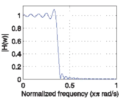
An ideal lowpass FIR digital owing an ideal response specification.

𝐻(𝑤) = {1⁡⁡⁡0 ≤ 𝑤 ≤ 𝑤𝑝 0⁡⁡⁡𝑤𝑠 ≤ 𝑤 ≤ 1

(1.22)

To achieve a minimum value of⁡δ, which is defined as

𝛿 = 𝑊(𝑤)|(𝐻(𝑤) − 𝐷(𝑤))| (1.23)

Where 𝑊⁡(𝑤), the weighting function can be expressed as

𝑊(𝑤) = {

1⁡⁡0 ≤ 𝑤 ≤ 𝑤_𝑝 0⁡⁡𝑤_𝑝 ≤ 𝑤 ≤ 𝑤_𝑠

1⁡⁡𝑤_𝑠 ≤ 𝑤 ≤ 1

(21)

7

1.6 Problem Formulation

An Nth-order non-recursive digital FIR filter can be represented by the transfer function

𝐻(𝑧) = ∑𝑁 ℎ_𝑛𝑧−𝑛_{= 𝒄}𝑇 𝑛=0

𝒛(𝑧) (1.25)

Where 𝒄𝑇 is real coefficients vector. N is the total number of filter coefficients. N-1 is its order. For optimization problem, the coefficients vector is

𝒄𝑇 _{= [𝑐}

1𝑐2… 𝑐𝑁] (1.26)

The frequency response can be gained by substituting 𝑧 = 𝑒𝑗𝑇𝑤, where 𝑇 is the sampling period in seconds and 𝑤 is the frequency.

For the design of a linear-phase FIR digital filter, assume 𝛺 = 𝑤_𝑖, 1 ≤ 𝑖 ≤ 𝑀, be the group of frequencies to evaluate the frequency response. Therefore, the error at each sample point in 𝑤_𝑖 is represented as

𝑒_𝑖 = 𝐻_𝑑(𝑤𝑖) − 𝐻(𝑤𝑖) (1.27)

Where 𝐻𝑑(𝑤𝑖) is the ideal digital filter frequency response and 𝐻⁡(𝑤𝑖) represents the actual frequency response of the designed filter. Because we only design symmetric FIR filter, the group delay is constant as defined as

𝜏 =𝑁

2 (1.28)

1.7 Coefficients initializing method

(22)

8 Fig. 1.3 Linear phase FIR filter coefficients initializing method

Experiment results show this can improve the convergence of optimizing progress.

𝑦 = exp⁡(𝑥) (1.29)

In this way, the convergence velocity becomes much faster than regular method.

1.8 Approximation Criteria

Minimax error designs

Minimax error function is defined as equation (1.30). It searches for the maximum peak ripple throughout a discrete frequency domain by subtracting the magnitude response of the ideal FIR filter to designed filter.

error = max{|𝐻_𝑑(𝑒𝑗𝜔)| − |𝐷(𝜔)|} (1.30)

Where 𝐷(𝜔) is the magnitude of the ideal filter, and 𝐻(𝑒𝑗𝑤𝑖₎ is the magnitude of the

designed filter. M is the number of frequency interval.

Least-Squared Error Designs.

Here, this error is defined as

𝐸𝑝 = ∫ [𝑊(𝜔)[|𝐻𝑑(𝑒𝑗𝜔)| − 𝐷(𝜔)]] 𝑝

𝑑𝜔 𝑋

(1.31)

(23)

9

𝐸₂ = ∫ [𝑊(𝜔)[|𝐻_𝑑(𝑒𝑗𝜔)| − 𝐷(𝜔)]]2𝑑𝜔 𝑋

(1.32)

1.9 Fitness function

As mentioned before, the error norm is used as the fitness function in our experiment. Therefore, the problem is transferred to optimize the coefficients by minimizing the error norms, i.e. error function.

Passband/stopband ripples

Passband/ stopband ripples are often expressed in dB,

Passband ripple = 20𝑙𝑜𝑔₁₀(1 + 𝛿_𝑝) dB,

Minimum stopband attenuation=-20𝑙𝑜𝑔10(𝛿𝑝) Db

1.10 Conclusion

This section introduces the basic knowledge on digital FIR filter design and concepts associated. The four types of symmetric digital filters are most commonly applied in this field, and some relevant methods are also explored. Coefficients optimization is the main and high-effective aspect by which specifications can be satisfied. Also, the cost function is introduced here. Minimax design technique is easy to complete, and the results obtained is superior as compared to other methods.

(24)

10

Chapter 2 Linear Phase Digital FIR Filter Design Using

PSO Algorithm

2.1. Particle Swarm Optimization

Currently, there are many approaches to FIR filter design, such as window functions, frequency sampling method and best uniform approximation. These methods are all based on the approximation to frequency characteristics of ideal FIR filters. Researchers recently have proposed Simulated Annealing Approach (SA) [6] and Genetic Algorithms (GA) [7]. As we know, GA is difficult to realize due to the complexity of coding and SA costs too much computation. PSO is a random search algorithm and has been successfully applied to many real-world problems.

PSO algorithm is one of the population-based stochastic algorithms for searching optimal solutions which is based on social-psychological principles. Unlike DE algorithm, it does not use selection strategy, typically, all population individuals survive from the beginning and update until the end. During that process, the quality of individuals can be improved by their interactions over time [8].

PSO was first presented in 1995 by James Kennedy and Russell C. Eberhart. PSO simulates a kind of social optimization in the animal swarm like ant group or fish schooling. Such a problem is given, and respondent methods to evaluate a proposed solution to it are in the form of a fitness function. Like the behavior in the group such as communication structure or social network are also defined, and neighbors can interact with the other particles. Then a population of individuals defined randomly at the problem solutions is initialized. These are candidate solutions exit in the objective space. These candidate solutions will be updated during the iterative process. The fitness of the candidate solutions and their positions are also remembered, and they are all available to their neighbors. It is convenient to choose a better candidate in each population.

Usually, a vector of D dimensions is randomly initialized in a specified space, is conceptualized as a point in a high-dimensional Cartesian coordinate system [8]. These points which are called particles can move around in the space. They often operate simultaneously and have the ability to convergence towards one direction within the searching space like animals behaviors, so that they are referred to as particle swarm. Comparing to Jehad I. Ababneh [23], we designed some more complex and higher dimensional linear phase digital FIR filters in this chapter.

(25)

11 searching a better way to find the food. [9]

PSO learns the knowledge itself from the iteration progress and solves the optimization problem. All the particles have fitness values which are calculated by the fitness function for optimization and have velocities to direct their step towards the objective solutions.

Define the solution space, fitness function,

and population size

Initialize positoin x, velocity v, local best and

global best

For every pariticle do

Update velocity v

Update position x

Recalculate fitness values

If fitness(x)<fitness(pbest), Pbest=current x If fitness(x)<fitness(gbest),

gbest=current x Next particle

Optimal solution Iteration condition

meet? Next

iteration

Yes No

Fig. 2.1 Flow chart of the PSO algorithm

(26)

12 other optimal solution is called the global optima which is the particle achieved the best fitness of all the population until now.

Normally, there are two characteristics which are used to represent the particle in the swarm:

1. The current position

2. The current velocity

The populations updated themselves according to the change of their position and velocity. These two vectors can be calculated by the following equations:

𝑣_𝑖𝑘+1= 𝑤𝑣_𝑖𝑘+ 𝑐₁𝑟₁(𝑝𝑏𝑒𝑠𝑡_𝑖− 𝑠_𝑖𝑘) + 𝑐₂𝑟₂(𝑔𝑏𝑒𝑠𝑡 − 𝑠_𝑖𝑘) (2.1)

𝑠_𝑖𝑘+1= 𝑠_𝑖𝑘+ 𝑣_𝑖𝑘+1 (2.2)

𝑣_𝑖𝑘 is the current velocity of 𝑖 at iteration 𝑘, 𝑠_𝑖𝑘 is the current position of 𝑖 at iteration 𝑘. 𝑐1 and 𝑐2 are two positive constants and 𝑟1 and 𝑟2 are random numbers between [0, 1].

The velocity value is limited to the range of [-𝑉𝑚𝑎𝑥,⁡𝑉𝑚𝑎𝑥].

The velocities of particles on each generation are constrained to a maximum. If a random acceleration makes the velocity on that iteration go beyond the maximum velocity, then the velocity on that generation is set to 𝑉𝑚𝑎𝑥. On the other side, if the reduction is less than

-𝑉𝑚𝑎𝑥, then it will be set to −𝑉𝑚𝑎𝑥. In this way, an unacceptable information lost will be forbidden during the mutation process.

The algorithm evaluates the particles vector in each generation in the fitness value 𝑓⁡(𝑥)

and compares the result to the best vector which is called 𝑝𝑏𝑒𝑠𝑡_𝑖 attained until now. If the current result is better than 𝑝𝑏𝑒𝑠𝑡_𝑖 so far, the vector 𝑝_𝑖 is updated with the current position

𝑠𝑖, and the previous best function result 𝑝𝑏𝑒𝑠𝑡𝑖 is updated with the current result.

The particles are always updated along with iterations within the region centered on the centroid of the current best 𝑝𝑏𝑒𝑠𝑡_𝑖 and 𝑔𝑏𝑒𝑠𝑡_𝑖. While it also gives an opportunity for the individuals to explore new space around the best values. After a lot of calculations, the particles will converge to optimal solutions, and the optimal fitness is obtained as well.

To implement PSO to solve the filter design, the filter coefficients {ℎ(0), ℎ(1), … , ℎ(𝑁 − 1)} represent the position of the particle.

The pseudo code of the procedure for designing a linear phase digital FIR filter is as follows:

𝐹𝑜𝑟⁡𝑒𝑎𝑐ℎ⁡𝑔𝑟𝑜𝑢𝑝⁡𝑜𝑓⁡𝑐𝑜𝑒𝑓𝑓𝑖𝑐𝑖𝑒𝑛𝑡𝑠 𝐷𝑂⁡{𝐼𝑛𝑖𝑡𝑖𝑎𝑙𝑖𝑧𝑒⁡𝑝𝑜𝑝𝑢𝑙𝑎𝑡𝑖𝑜𝑛

}

𝐷𝑜{

⁡𝐹𝑜𝑟⁡𝑒𝑎𝑐ℎ⁡𝑝𝑜𝑝𝑢𝑙𝑎𝑡𝑖𝑜𝑛{

(27)

13

⁡𝐼𝑓⁡𝑡ℎ𝑒⁡𝑓𝑖𝑡𝑛𝑒𝑠𝑠⁡𝑣𝑎𝑙𝑢𝑒⁡𝑖𝑠⁡𝑏𝑒𝑡𝑡𝑒𝑟⁡𝑡ℎ𝑎𝑛⁡𝑡ℎ𝑒⁡𝑏𝑒𝑠𝑡⁡𝑓𝑖𝑡𝑛𝑒𝑠𝑠⁡𝑣𝑎𝑙𝑢𝑒⁡(𝑝𝐵𝑒𝑠𝑡)⁡𝑖𝑛⁡ℎ𝑖𝑠𝑡𝑜𝑟𝑦 ⁡𝑠𝑒𝑡⁡𝑐𝑢𝑟𝑟𝑒𝑛𝑡⁡𝑣𝑎𝑙𝑢𝑒⁡𝑎𝑠⁡𝑡ℎ𝑒⁡𝑛𝑒𝑤⁡𝑝𝐵𝑒𝑠𝑡

⁡ }

⁡𝐶ℎ𝑜𝑜𝑠𝑒⁡𝑡ℎ𝑒⁡𝑖𝑛𝑑𝑖𝑣𝑖𝑢𝑎𝑙⁡𝑤𝑖𝑡ℎ⁡𝑡ℎ𝑒⁡𝑏𝑒𝑠𝑡⁡𝑓𝑖𝑡𝑛𝑒𝑠𝑠⁡𝑣𝑎𝑙𝑢𝑒⁡𝑜𝑓⁡𝑎𝑙𝑙⁡𝑡ℎ𝑒⁡𝑝𝑎𝑟𝑡𝑖𝑐𝑙𝑒𝑠⁡𝑎𝑠⁡𝑡ℎ𝑒⁡𝑔𝐵𝑒𝑠𝑡 ⁡𝐹𝑜𝑟⁡𝑒𝑎𝑐ℎ⁡𝑖𝑛𝑑𝑖𝑣𝑖𝑑𝑢𝑎𝑙{

⁡𝐶𝑎𝑙𝑐𝑢𝑙𝑎𝑡𝑒⁡𝑖𝑛𝑑𝑖𝑣𝑖𝑑𝑢𝑎𝑙⁡𝑣𝑒𝑙𝑜𝑐𝑖𝑡𝑦⁡𝑎𝑐𝑐𝑜𝑟𝑑𝑖𝑛𝑔⁡𝑡𝑜⁡𝑒𝑞𝑢𝑎𝑡𝑖𝑜𝑛⁡(𝑎) ⁡𝑈𝑝𝑑𝑎𝑡𝑒⁡𝑖𝑛𝑑𝑖𝑣𝑖𝑑𝑢𝑎𝑙⁡𝑝𝑜𝑠𝑖𝑡𝑖𝑜𝑛⁡𝑎𝑐𝑐𝑜𝑟𝑑𝑖𝑛𝑔⁡𝑡𝑜⁡𝑒𝑞𝑢𝑎𝑡𝑖𝑜𝑛⁡(𝑏) ⁡ }

}While maximum iterations or minimum error criteria is not attained, repeat.

After finishing the optimizing process, an individual which has the best fitness value should be obtained in the form of {ℎ(0), ℎ(1), … , ℎ(𝑁 − 1)}

2.2 Fitness function

In PSO, the value of fitness function can judge the particle’s position whether it is ‘better.’ As mention above, we use the minimax error as the fitness function of FIR digital filter, that is

𝑓𝑖𝑡𝑛𝑒𝑠𝑠 = 𝐸 = max{𝐻(𝜔) − 𝐷(𝜔)} (2.3)

Where 𝐻(𝜔) is the frequency response of designed filter, and 𝐷⁡(𝜔) represents the frequency response of the ideal lowpass and highpass filters.

𝐻(𝑒𝑗𝑤_{) = {}1,⁡⁡⁡0 ≤ 𝑤 ≤ 𝑤𝑐

0, 𝑤_𝑐 ≤ 𝑤 ≤ 𝜋 (2.4)

𝐻(𝑒𝑗𝑤) = {0,⁡⁡⁡0 ≤ 𝑤 ≤ 𝑤_{1, 𝑤} 𝑐

𝑐 ≤ 𝑤 ≤ 𝜋 (2.5)

And for bandpass filter, the frequency response is

𝐻(𝑒𝑗𝑤) = {1,⁡⁡⁡𝑤𝑐1 ≤ 𝑤 ≤ 𝑤𝑐2

0,⁡⁡⁡⁡⁡⁡⁡⁡⁡⁡𝑒𝑙𝑠𝑒𝑤ℎ𝑒𝑟𝑒 (2.6)

And for bandstop filter, the frequency response is

𝐻(𝑒𝑗𝑤_{) = {}0,⁡⁡⁡𝑤𝑐1 ≤ 𝑤 ≤ 𝑤𝑐2

1,⁡⁡⁡⁡⁡⁡⁡⁡⁡⁡𝑒𝑙𝑠𝑒𝑤ℎ𝑒𝑟𝑒 (2.7)

(28)

14

2.3. Experiments and results

This section presents the simulations performed for the design of all four types, i.e., FIR LP, HP, BP and BS filters. Each filter order (N) is taken as 12, 24, 36, and 48 respectively. For the LP filter, passband (normalized) edge frequency 𝑤_𝑝=0.45; stopband (normalized) edge frequency 𝑤_𝑠=0.55; For the HP filter, stopband (normalized) edge frequency 𝑤_𝑝=0.45; passband (normalized) edge frequency 𝑤𝑝 =0.55; For the BP filter, lower stop band (normalized) edge frequency 𝑤_𝑠1 =0.25; lower passband (normalized) edge frequency

𝑤_𝑝1 =0.35; upper passband (normalized) edge frequency 𝑤_𝑝2 =0.6; upper stopband (normalized) edge frequency 𝑤_𝑠2=0.7. For the BS filter, lower passband (normalized) edge frequency 𝑤_𝑝1=0.3; lower stop band (normalized) edge frequency 𝑤_𝑠1=0.4; upper stopband (normalized) edge frequency 𝑤𝑠2 =0.55; upper passband (normalized) edge frequency 𝑤_𝑝2= 0.65.

The original population of each of filter examples are generated using the way which is introduced in the first chapter. We randomly select 7, 13, 19, 25 figures from [0, 1] and sort these figures as one side of the initial population of the odd-symmetric filters of 12th-order, 24th-order, 36th-order, and 48th-order, respectively. The opposite side of the filter coefficients is copied from these coefficients which are already produced using the above way. The size of the population is determined by the repeats of the above process.

The experiment works on Intel (R) Core i5-3210M, 2.50GHz, 8G RAM, Windows 10 and Matlab R2014a.

The example are divided to two part: one is simulated for type1, and the other part is for type2. Lowpass, highpass, bandpass, and bandstop filters are designed. Their frequency response is as follows:

Maximum velocity=1, 𝑤_𝑚𝑎𝑥= 1, 𝑤_𝑚𝑖𝑛 = 0.5, 𝑐₁ = 2, 𝑐₂ = 2, 𝑟_𝑓 = 1, 𝑟_𝑔 = 1

2.3.1 Type1 lowpass linear phase digital FIR filter

Type1 lowpass FIR filter with order 12

Table 2.1 Coefficients of 12th-order type1 LP-FIR filter by PSO

h(n) coefficients h(n) coefficients

h(1) = h(13) 0.005534994356476 h(4) = h(10) -0.210273228457961

h(2) = h(12) 0.204903829885383 h(5) = h(9) 0.002978951624785

h(3) = h(11) -0.002359268425988 h(6) = h(8) 0.633865285274643

h(7) 0.979474555157335

The computational time, passband and stopband ripple error of the linear phase digital FIR filter design with PSS algorithm is showed in Table 2.2, respectively.

Table 2.2 Design result of 12th-order LP-FIR filter by PSO

(29)

15

144.075300 0.151279546816109 0.150398090335351

The magnitude responses of the linear phase digital FIR filters designed using the PSO algorithms for the filter of are given in Fig 2.2.

The figure on the right shows the magnitude response in dB, the local details of the passband, its group delay, and phase features.

Fig. 2.2 Magnitude, ripple errors of 12th-order LP-FIR filter by PSO

h(1) = h(25) -0.00205313558952449 h(8) = h(18) 0.0562946888009923

h(2) = h(24) -0.030068149381552 h(9) = h(17) -0.000581504493755191

h(3) = h(23) -0.00147132225764667 h(10) = h(16) -0.10145624481207

h(4) = h(22) 0.0260337333074784 h(11) = h(15) -0.00176296327102027

h(5) = h(21) 0.00206282005990487 h(12) = h(14) 0.31798107800902

h(6) = h(20) -0.0399928058440625 h(13) 0.498109088452561

h(7) = h(19) 0.00261279638810157

The computational time, passband and stopband ripple error of the linear phase digital FIR filter design with POS algorithm is showed in Table 2.4, respectively.

Time/s Stopband error Passband error

172.832061 0.046248431572409 0.053365558441687

(30)

16 Fig. 2.3 Magnitude, ripple errors of 24th-order LP-FIR filter by PSO

Type1 lowpass order 36

h(1) = h(37) -0.000848687622753 h(11) = h(27) 0.005178935904278

h(2) = h(36) -0.014373261726844 h(12) = h(26) 0.070252878147661 h(3) = h(35) 0.003532976138188 h(13) = h(25) -0.004009188000524

h(4) = h(34) 0.020972225219487 h(14) = h(24) -0.113059749018623

h(5) = h(33) 0.000261333849933 h(15) = h(23) 0.000922838929777

h(6) = h(32) -0.024552465492260 h(16) = h(22) 0.196319899422876

h(7) = h(31) 0.003499169897124 h(17) = h(21) -0.005800980449815

h(8) = h(30) 0.036518218751672 h(18) = h(20) -0.608830155468197

h(9) = h(29) -0.004067059332583 h(19) -0.949698223596581

h(10) = h(28) -0.052709642218845

406.050082 0.016303333542335 0.016968828284386

(31)

h(1) = h(49) -0.001047264802628 h(14) = h(36) -0.034660689509657

h(2) = h(48) -0.004659896562826 h(15) = h(35) 0.004719266242802 h(3) = h(47) 0.003306790794211 h(16) = h(34) 0.046425707658136

h(4) = h(46) 0.00581997949029 h(17) = h(33) -0.006608506408141

h(5) = h(45) -0.002073757257038 h(18) = h(32) -0.062984244647794

h(6) = h(44) -0.009249000318886 h(19) = h(31) 0.006155543726317

h(7) = h(43) 0.003448015255106 h(20) = h(30) 0.095378325180374

h(8) = h(42) 0.013281408303607 h(21) = h(29) -0.007321790729720

h(9) = h(41) -0.004504414159347 h(22) = h(28) -0.166505155145664

h(10) = h(40) -0.016130603174843 h(23) = h(27) 0.007741285042549

h(11) = h(39) 0.002097831633416 h(24) = h(26) 0.510589821652021

h(12) = h(38) 0.022569671716071 h(25) 0.793783575156937

h(13) = h(37) -0.005590606138566

2617.883373 0.0073759340395515 0.0073776557844607

(32)

Fig. 2.6 Convergence behaviors of PSO in design LP-FIR with orders of 12th, 24th, 36th, and 48th

2.3.2. Type1 Highpass linear phase digital FIR filter

Type1 Highpass linear phase digital FIR filter with order 12

Table 2. 9 Coefficients of 12th-order type1 HP-FIR filter by PSO

h(1) = h(13) 0.000699867644626 h(4) = h(10) -0.208747738841508

(33)

19 h(3) = h(11) -0.000955508310356 h(6) = h(8) 0.624370820348988

h(7) -0.975158774797411

Table 2. 10 Design result of 12th-order HP-FIR filter by PSO

34.558574 0.149579872844649 0.152893741918110

Fig. 2.7 Magnitude, ripple errors of 12th HP-FIR lowpass filter by PSO

Type 1 highpass linear phase digital FIR filter with order 24

Table 2.11 Coefficients of 24th-order type1 HP-FIR filter by PSO

h(1) = h(25) -0.001907719929447 h(8) = h(18) 0.107553738673346

h(2) = h(24) -0.055324456754076 h(9) = h(17) -0.002029337109109

h(3) = h(23) 0.002978848699407 h(10) = h(16) -0.197381510034050

h(4) = h(22) 0.054053250962448 h(11) = h(15) 0.006846698762999

h(5) = h(21) -0.005152605134815 h(12) = h(14) 0.611147624673500

h(6) = h(20) -0.072714988789047 h(13) -0.963200080999353

h(7) = h(19) 0.003124128814972

The computational time, passband and stopband ripple error of the linear phase digital FIR filter design with POS algorithm is showed in Table 2.12, respectively

Table 2.12 Design result of 24th-order HP-FIR filter by PSO

(34)

20

431.147374 0.045813959055968 0.045990750663258

Fig. 2.8 Magnitude, ripple errors of 24th-order HP-FIR filter by PSO

h(1) = h(37) 0.000257940835591 h(11) = h(27) -0.004614175665226

h(2) = h(36) 0.015851822991697 h(12) = h(26) -0.076993982614866 h(3) = h(35) -0.000491936905874 h(13) = h(25) -0.000225186192316

h(4) = h(34) -0.020685296757903 h(14) = h(24) 0.116684493870300

h(5) = h(33) 0.003804097208211 h(15) = h(23) -0.004807348118044

h(6) = h(32) 0.027935193987771 h(16) = h(22) -0.203959876121314

h(7) = h(31) 0.000218954155286 h(17) = h(21) 0.002424322968095

h(8) = h(30) -0.036723866724770 h(18) = h(20) 0.631109560654634

h(9) = h(29) 0.003909211381214 h(19) -0.999636331503199

h(10) = h(28) 0.053262003380551

395.028087 0.015911927701090 0.016021904562858

(35)

21 Fig. 2.9 Magnitude, ripple errors of 36th-order HP-FIR filter by PSO

h(1) = h(49) -0.000603441469539 h(14) = h(36) -0.040673064911518

h(2) = h(48) -0.006267240220903 h(15) = h(35) 0.002990087861222 h(3) = h(47) 0.000882865918032 h(16) = h(34) 0.055846976629837

h(4) = h(46) 0.008148050131759 h(17) = h(33) -0.003693795258497

h(5) = h(45) -0.001839497968108 h(18) = h(32) -0.078841933621902

h(6) = h(44) -0.010526362466545 h(19) = h(31) 0.004421671842661

h(7) = h(43) 0.001265204169247 h(20) = h(30) 0.117417322608263

h(8) = h(42) 0.016199629333704 h(21) = h(29) -0.003699979773455

h(9) = h(41) -0.002210154896543 h(22) = h(28) -0.204014489335479

h(10) = h(40) -0.021937089750019 h(23) = h(27) 0.004587720204273

h(11) = h(39) 0.002346245169983 h(24) = h(26) 0.625918538674400

h(12) = h(38) 0.029893743977659 h(25) -0.990087899311546

h(13) = h(37) -0.003288283096666

4438.526250 0.005342504707092 0.005322669623213

(36)

22 Fig. 2.10 Magnitude, ripple errors of 48th-order HP-FIR filter by PSO

Fig. 2.11 Convergence behaviors of PSO in design HP-FIR with orders of 12th, 24th, 36th, and 48th

2.3.3. Type1 Bandpass linear phase digital FIR filter

Type1 Bandpass linear phase digital FIR filter with order 12

Table 2.17 Coefficients of 12th-order type1 BP-FIR filter by PSO

(37)

23 h(3) = h(11) 0.149374001755597 h(6) = h(8) 0.0476680091323586

h(7) 0.378345935579198

Table 2.18 Design result of 12th-order BP-FIR filter by PSO

147.013430 0.186476983648942 0.208422639560898

Fig. 2.12 Magnitude, passband and stopband errors of 12th-order BP-FIR lowpass filter

Type 1 bandpass linear phase digital FIR filter with order 24

h(1) = h(25) -0.022831234638210 h(8) = h(18) -0.051825209777017

h(2) = h(24) -0.013210758361870 h(9) = h(17) -0.328946451064623

h(3) = h(23) -0.079511782200070 h(10) = h(16) 0.155022612546842

h(4) = h(22) 0.104970109564400 h(11) = h(15) 0.826929849162887

h(5) = h(21) 0.136964193758678 h(12) = h(14) -0.059169805097528

h(6) = h(20) -0.089474043268753 h(13) -0.996832368860821

h(7) = h(19) -0.033363721334422

(38)

24

215.402234 0.061758283413739 0.063718444449077

The magnitude responses of the linear phase digital FIR filters designed using the PSO, PSO algorithms for the filter of are given in Fig 2.13.

Fig. 2.13 Magnitude, ripple errors of 24th-order BP-FIR filter by PSO

h(1) = h(37) -0.000505428202119794 h(11) = h(27) -0.0464646850831868

h(2) = h(36) -0.00281619589815389 h(12) = h(26) 0.0322793100346188 h(3) = h(35) 0.000610846544854953 h(13) = h(25) 0.0154005739825305

h(4) = h(34) -0.0191331357877065 h(14) = h(24) 0.0184805956704867

h(5) = h(33) -0.00717224237784085 h(15) = h(23) 0.110752571969189

h(6) = h(32) 0.020567172970441 h(16) = h(22) -0.05511145997133

h(7) = h(31) 0.00743666122569187 h(17) = h(21) -0.277403463772834

h(8) = h(30) 0.0034297177512027 h(18) = h(20) 0.0292053587486496

h(9) = h(29) 0.0191099865744274 h(19) 0.356195418739576

h(10) = h(28) -0.0379904435590879

431.318895 0.0228430634111649 0.0370987264169751

(39)

25 Fig. 2.14 Magnitude, ripple errors of 36th-order BP-FIR filter by PSO

h(1) = h(49) -0.001618373921611 h(14) = h(36) 0.022259478588033

h(2) = h(48) -0.001950510667381 h(15) = h(35) 0.065611290125299 h(3) = h(47) -0.002558648107667 h(16) = h(34) -0.106846864275660

h(4) = h(46) -0.017722790997972 h(17) = h(33) -0.141188237958171

h(5) = h(45) 0.002079850886173 h(18) = h(32) 0.080731455266420

h(6) = h(44) 0.026636485822660 h(19) = h(31) 0.036321081289342

h(7) = h(43) 0.000792983850795 h(20) = h(30) 0.053380247329694

h(8) = h(42) 0.004335209850867 h(21) = h(29) 0.332597512079348

h(9) = h(41) 0.007503070213622 h(22) = h(28) -0.145446727933191

h(10) = h(40) -0.054146624068345 h(23) = h(27) -0.790748394588430

h(11) = h(39) -0.027369381119378 h(24) = h(26) 0.079765300554222

h(12) = h(38) 0.056553279439342 h(25) 0.997926201265134

h(13) = h(37) 0.016730690361832

3738.516128 0.006662125873949 0.006669725210366

(40)

26 Fig. 2.15 Magnitude, ripple errors of 24th-order BP-FIR filter by PSO

Fig. 2.16 Convergence behaviors of PSO in design BP-FIR with orders of 12th, 24th, 36th, and 48th

2.3.4. Type1 Bandstop linear phase digital FIR filter

Type 1 Bandstop linear phase digital FIR filter with order 12

Table 2.25 Coefficients of 12th-order type1 BS-FIR filter by PSO

(41)

27 h(3) = h(11) -0.155838698632166 h(6) = h(8) -0.0242971361994448

h(7) 0.75125472351821

Table 2.26 Design result of 12th-order BS-FIR filter by PSO

842.874272 0.107590998821996 0.163215646048442

Fig. 2.17 Magnitude, ripple errors of 12th-order BS-FIR filter by PSO

Type 1 bandstop linear phase digital FIR filter with order 24

h(1) = h(25) -0.010041643905328 h(8) = h(18) -0.073108749021779

h(2) = h(24) 0.008752099017537 h(9) = h(17) 0.003874843950236

h(3) = h(23) -0.046154207062890 h(10) = h(16) -0.128901644993284

h(4) = h(22) -0.054018306619055 h(11) = h(15) 0.055099357284101

h(5) = h(21) 0.055800717510152 h(12) = h(14) 0.948686432340606

h(6) = h(20) 0.098450746325749 h(13) -0.098563580368962

h(7) = h(19) -0.052583358491048

(42)

28

619.408664 0.060703136028247 0.059849388853956

Fig. 2.18 Magnitude, ripple errors of 24th-order BS-FIR filter by PSO

h(1) = h(37) 0.017773874586921 h(11) = h(27) 0.071488794603505

h(2) = h(36) 0.001358913804423 h(12) = h(26) 0.099192906544670 h(3) = h(35) -0.031103805366174 h(13) = h(25) -0.055278314979214

h(4) = h(34) -0.011038198368998 h(14) = h(24) -0.056801273948647

h(5) = h(33) 0.019636917755613 h(15) = h(23) -0.007673251726469

h(6) = h(32) 0.005196694103630 h(16) = h(22) -0.141106459476036

h(7) = h(31) 0.006304187674171 h(17) = h(21) 0.070004788584924

h(8) = h(30) 0.025301612786365 h(18) = h(20) 0.991911540626346

h(9) = h(29) -0.045480389649695 h(19) -0.093920328972359

h(10) = h(28) -0.064897559056597

738.516128 0.020408839055092 0.023572479676884

(43)

29 Fig. 2.19 Magnitude, ripple errors of 36th-order BS-FIR filter by PSO

h(1)= h(49) -0.000169704101268 h(14)= h(36) 0.040923016277587 h(2)= h(48) -0.002204526890458 h(15)= h(35) 0.028142078783271 h(3)= h(47) 0.001145023600625 h(16)= h(34) -0.019351053472599 h(4)= h(46) 0.008965859010271 h(17)= h(33) 0.002463417125072 h(5)= h(45) -0.001773679137716 h(18)= h(32) -0.024925849525594 h(6)= h(44) -0.013633565384252 h(19)= h(31) -0.080217909596378 h(7)= h(43) -0.000562151020954 h(20)= h(30) 0.061815100463508 h(8)= h(42) 0.005274843402903 h(21)= h(29) 0.189943507899946 h(9)= h(41) -0.001095910503299 h(22)= h(28) -0.064809608668370 h(10)= h(40) 0.012215261004327 h(23)= h(27) -0.290064707351143 h(11)= h(39) 0.008397866441987 h(24)= h(26) 0.028674685088707 h(12)= h(38) -0.033560659786482 h(25) -0.999614460016997 h(13)= h(37) -0.022828339160021

1118.671875 0.007381528454473 0.007252200677178

(44)

Fig. 2.21 Convergence behaviors of PSO in design BS-FIR with orders of 12th, 24th, 36th, and 48th

(45)

31 limit to apply in the designing of linear phase digital FIR filters.

In the next part, we designed two types of linear phase digital FIR filters which are lowpass and bandpass filters all with order 25 and 49. The parameters are same with before.

2.3.5 Type 2 lowpass linear phase digital FIR filter

This section presents the simulations performed for the design of two type 2 linear phase digital filters of LP and BP. Each filter order (N) is taken as 25 and 49 respectively. For the LP filter, passband (normalized) edge frequency 𝑤𝑝 =0.45; stopband (normalized) edge frequency 𝑤_𝑠 =0.55; For the BP filter, lower stop band (normalized) edge frequency

𝑤_𝑠1 =0.25; lower passband (normalized) edge frequency 𝑤_𝑝1 =0.35; upper passband (normalized) edge frequency 𝑤_𝑝2 =0.6; upper stopband (normalized) edge frequency

𝑤_𝑠2=0.7.

The original populations of each filter example are generated using the way which is similar to the type1 filter design. We randomly select 13, 25 figures from [0, 1] and sort these figures as one side of the initial population of the even symmetric filter of 25th-order and 49th-order, respectively. During the optimization process, the other side of the coefficients will be copied from the existing part.

Type 2 lowpass linear phase digital FIR filter of order 25

h(1) = h(26) 0.021970049995995 h(8) = h(19) 0.082335959350398

h(2) = h(25) -0.042272763743529 h(9) = h(18) 0.103866164049824

h(3) = h(24) -0.032531084894305 h(10) = h(17) -0.128142059153321

h(4) = h(23) 0.037341010410492 h(11) = h(16) -0.180423644142344 h(5) = h(22) 0.042498398732192 h(12) = h(15) 0.321345127863449

h(6) = h(21) -0.057245976097162 h(13) = h(14) 0.963366910397667

h(7) = h(20) -0.061658345456958

Table 2.34 Design result of 25th-order type 2 LP-FIR filter by PSO

2337.243058 0.041201848758123 0.041827017886749

(46)

32 Fig. 2.22 Magnitude, ripple errors of 25th-order type2 LP-FIR filter by PSO

Type 2 lowpass linear phase digital FIR filter of order 49

h(1) = h(50) 0.006133118233681 h(14) = h(37) -0.028993261817678

h(2) = h(49) -0.003915934995176 h(15) = h(36) -0.036547454718272

h(3) = h(48) -0.006571712845000 h(16) = h(35) 0.040315607310961

h(4) = h(47) 0.003328196544599 h(17) = h(34) 0.048766636234117

h(5) = h(46) 0.006043747413523 h(18) = h(33) -0.056466921677217

h(6) = h(45) -0.007475530660646 h(19) = h(32) -0.070307616619783

h(7) = h(44) -0.011715760628665 h(20) = h(31) 0.083980461774395

h(8) = h(43) 0.010091974525746 h(21) = h(30) 0.108472348438981

h(9) = h(42) 0.014564232870161 h(22) = h(29) -0.137012274576683 h(10) = h(41) -0.016197555729881 h(23) = h(28) -0.199552203474627

h(11) = h(40) -0.021298473430499 h(24) = h(27) 0.328834975057105

h(12) = h(39) 0.021332519373483 h(25) = h(26) 0.999999995619789

h(13) = h(38) 0.026643157781947

Linear Phase FIR Digital Filter Design Using Differential Evolution Algorithms

Scholarship at UWindsor

Scholarship at UWindsor

Linear Phase FIR Digital Filter Design Using Differential Evolution

Linear Phase FIR Digital Filter Design Using Differential Evolution

Algorithms

Algorithms

Linear Phase FIR Digital Filter Design Using Differential Evolution

Algorithms

by

Wei Zhong

A Thesis

Submitted to the Faculty of Graduate Studies

through Electrical and Computer Engineering

in Partial Fulfillment of the Requirements for

the Degree of Master of Applied Science at the

University of Windsor

Windsor, Ontario, Canada

2016

Linear Phase FIR Digital Filter Design Using Differential Evolution

Algorithms

by

Wei Zhong

APPROVED BY:

______________________________________________

Dr. Z. Kobti

School of Computer Science

______________________________________________

Dr. Huapeng Wu

Department of Electrical & Computer Engineering

______________________________________________

Dr. H. K. Kwan, Advisor

Department of Electrical and Computer Engineering

______________________________________________

Declaration of Originality

Abstract

Acknowledgements

Table of Contents

List of Tables

List of Figures

List of Abbreviations

Chapter 1 Introduction to Linear Phase Digital FIR

Filter Design

1.1 Introduction

1.2 FIR digital filter

1.3 Symmetric Filters

1.4 Linear phrase filters

1.5 Digital FIR filter design

1.6 Problem Formulation

1.7 Coefficients initializing method

1.8 Approximation Criteria

1.9 Fitness function

1.10 Conclusion

Chapter 2 Linear Phase Digital FIR Filter Design Using

PSO Algorithm

2.1. Particle Swarm Optimization

2.2 Fitness function

2.3. Experiments and results