Two dimensional determination of source terms in linear parabolic equation from the final overdetermination

(1)

R E S E A R C H

Open Access

Two dimensional determination of source

terms in linear parabolic equation from the

ﬁnal overdetermination

Xiujin Miao

1*

_{and Zhenhai Liu}

1,2

*_{Correspondence:}

[email protected]

1_{School of Mathematics and}

Statistics, Central South University, No. 22 South Shaoshan Road, Changsha, 410075, P.R. China Full list of author information is available at the end of the article

Abstract

A case of steady-case heat ﬂow through a plane wall, which can be formulated as

ut(x,y,t) – div(k(x,y)∇u(x,y,t)) =F(x,y,t) with Robin boundary condition –k(1,y)ux(1,y,t) =

ν

1[u(1,y,t) –T0(t)], –k(x, 1)uy(x, 1,t) =

ν

2[u(x, 1,t) –T1(t)], where

ω

:={F(x,y,t);T0(t);T1(t)}is to be determined, from the measured ﬁnal data

μ

T(x,y) =u(x,y,T) is investigated. It is proved that the Fréchet gradient of the cost

functionalJ(

ω

) =

μ

T(x,y) –u(x,y,T;

ω

)2can be found via the solution of the adjoint

parabolic problem. Lipschitz continuity of the gradient is derived. The obtained results permit one to prove the existence of a quasi-solution of the inverse problem. A steepest descent method with line search, which produces a monotone iteration scheme based on the gradient, is formulated. Some convergence results are given.

Keywords: two dimensional determination; cost functional; steepest descent method

1 Introduction

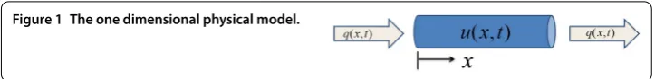
Consider the one dimensional physical system in Figure , where the left of the solid is full of hot gas. Whenever a temperature gradient exists in the solid medium, heat will ﬂow from the higher-temperature region to the lower-temperature region. According to

Fourier’s law, for a homogeneous, isotropic solid, the following equation holds:

q(x,t) = –kuxx(x,t), (.)

whereq(x,t) represents heat ﬂow per unit time, per unit area of the isothermal surface in the direction of decreasing temperature,u(x,t) is the temperature distribution in the solid, andkis called the thermal conductivity.

However, in practice, the thermal conductivity may depend onx, namely,k:=k(x). Be-sides, there may be a heat sourceg(x,t) in the solid. Under these conditions, the physical system can be formulated as

⎧ ⎪ ⎨ ⎪ ⎩

ut= (k(x)ux(x,t))x+g(x,t), (x,t)∈ ˜T, u(x, ) =μ(x), x∈(,L),

ux(,t) = , –k(L)ux(L,t) =σ[u(L,t) –T(t)], t∈(,T],

(.)

(2)

Figure 1 The one dimensional physical model.

where˜T:={ <x<L,  <t≤T}, andT(t) is the temperature of the cold gas on the

right of the solid. –k(L)ux(L,t) =σ[u(L,t) –T(t)] represents the convection atx=L

according toNewton’s law, and the constantσis called the convection coefficient. It is desired to find the pairω:={g(x,t);T(t)}from the final state observation

μT(x) =u(x,T). (.)

The mathematical model (.) can also arise in hydrology [], material sciences [], and transport problems []. In [] a tsunami model based on shallow water theory is studied. The authors treat the inverse problem of determining an unknown initial tsunami source

q(x,y) by using measurementsfm(t) of the height of a passing tsunami wave at a ﬁnite number of given points (xm,ym),m= , , . . . ,M, of the coastal area. These are nonlinear inverse problems, and it is well known that they are generally ill posed,i.e.the existence, uniqueness, and stability of their solutions are not always guaranteed []. There are many contributions for the linear parabolic equations with ﬁnal overdetermination (see, for in-stance [–]). The time-dependent heat sourceH(t) of the separable sources of the form

g(x,t) =F(x)H(t) is investigated in []. Forg(x,t) =p(x)u, in [], the author proved the existence and uniqueness ofp(x), and the local well-posedness of the inverse problem was discussed in []. The simultaneous reconstruction of the initial temperature and heat ra-diative coefficient was investigated in [] by using the measurement of temperature given at a fixed time and the measurement of the temperature in a subregion of the physical do-main. A determination of the unknown functionp(x) in the source termg=p(x)f(u), via fixed point theory, was given in []. Based on the optimal control framework, [] con-sidered the determination of a pair (p,u) in the nonlinear parabolic equation

ut–uxx+p(x)f(u) = ,

with initial and homogeneous Dirichlet boundary conditions:

u(x, ) =φ(x), u|x==u|x=L= ,

from the overspeciﬁed datau(x,T) =μT(x). The local uniqueness and stability of the

so-lution were proved. In [], a weak soso-lution approach for the pairω(x,t) :={g(x,t);T(t)}

was given via a steepest descent method on minimizing the cost functional

J(ω) =μT(x) –u(x,T;ω)



(3)

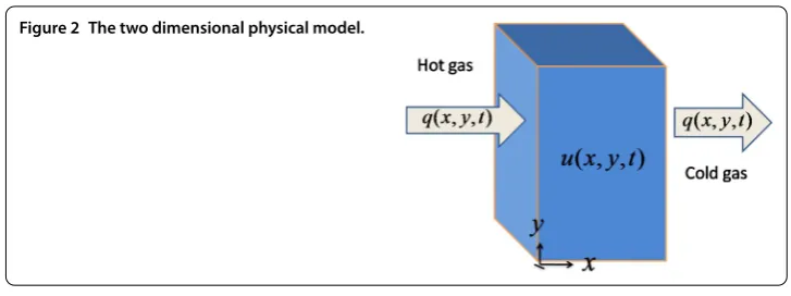
Figure 2 The two dimensional physical model.

In this contribution, we consider the corresponding two dimensional problem (see Fig-ure ) as follows:

⎧ ⎪ ⎪ ⎪ ⎪ ⎪ ⎪ ⎨ ⎪ ⎪ ⎪ ⎪ ⎪ ⎪ ⎩

ut(x,y,t) –div(k(x,y)∇u(x,y,t)) =F(x,y,t), inT,

ux(,y,t) =uy(x, ,t) = , x,y∈(, ),t∈(,T], –k(,y)ux(,y,t) =ν[u(,y,t) –T(t)], x,y∈(, ),t∈(,T],

–k(x, )uy(x, ,t) =ν[u(x, ,t) –T(t)], x,y∈(, ),t∈(,T],

u(x,y, ) =u(x,y), (x,y)∈,

(.)

whereT=×(,T) = (, )×(, )×(,T) andν,ν> . The inverse problem here is

to determineω:={F(x,y,t);T(t);T(t)}from the ﬁnal state observation (the overspeciﬁed

data)

uT(x,y) =u(x,y,T). (.) In this work, based on a weak solution approach we will show how the inverse problem can be formulated and solved forω:={F(x,y,t);T(t);T(t)}. Moreover, we will prove that

the gradientJ(w) of the cost (auxiliary) functional

J(ω) =μT(x,y) –u(x,y,T;ω)



can be expressed via the solutionϕ=ϕ(x,y,t;ω) of the appropriate adjoint problem. This paper is organized as follows. In Section , we give an analysis of the two dimen-sional problem and prove the Fréchet-diﬀerentiability ofJ(ω). In Section , we present the framework of a steepest descent iterate with line search of the two dimensional inverse problem, whereJ(ω) can be found via an adjoint parabolic problem. The convergence of the sequence is analyzed in Section . Conclusions are stated in Section .

2 The analysis of the two dimensional problem

The direct problem (.) is to get the solution from a given pairw. Firstly, we deﬁneW:=

F×T×T, the set of admissible unknown sourcesF(x,y,t),T(t),T(t) with

F(x,y,t)∈L(T), T(t),T(t)∈L[,T],

 <T∗≤T(t),T(t)≤T∗< +∞,

(.)

(4)

It is obvious that the setWis a closed and convex subset inL₍

T)×L[,T]×L[,T].

The scalar product inWis deﬁned as

(ω,ω)W:=

T

F(x,y,t)F(x,y,t)dx dy dt+

T



T_()(t)T_()(t)dt

+

T



T_()(t)T_()(t)dt, ∀ω,ω∈W,

whereωm:={Fm;T(m);T (m)

 },m= , . We can prove that this kind of problem has a

quasi-solutionu∈H,₍

T) satisfying the identity

u(x,y,T)v(x,y,T)dx dy–

u(x,y)v(x,y, )dx dy

–

T

(uvt–kuxvx–kuyvy)dx dy dt

=ν

T







u(,y,t) –T(t)v(,y,t)dy dt

+ν

T







u(x, ,t) –T(t) v(x, ,t)dx dt+

T



F(x,y,t)v(x,y,t)dx dt, (.)

for allv∈H,(T). HereH,(T) is the Sobolev space with the norm

u:=

T

u+u_x+u_y dx dy dt /

.

It is also known that, under conditions (.) and (.), the weak solution u(x,y,t)∈

H,₍

T) of the direct problem (.) exists and is unique [].

2.1 Method discussion

To solve the inverse problem (.)-(.), we introduce a cost functional

J(ω) =

u(x,y,T;ω) –uT(x,y) dx dy.

We are going to give an iterative solution to this kind of problem. To begin, we study the derivative of the cost functional. Let us consider the ﬁrst variation of the cost functional:

J(ω) :=J(ω+ω) –J(ω) =

u(x,y,T;ω+ω) –uT(x,y)dx dy–

u(x,y,T;ω) –uT(x,y)dx dy

=

u(x,y,T;ω)u(x,y,T;ω) + u(x,y,T;ω) –uT(x,y)dx dy

= 

u(x,y,T;ω) –uT(x,y)u(x,y,T;ω)dx dy

+

(5)

where

ω+ω:={F+F;T+T;T+T} ∈W,

u(x,y,t;ω) :=u(x,y,t;ω+ω) –u(x,y,t;ω)∈H,(T).

Furthermore, the functionu:=u(x,y,t;ω) is the solution of the following parabolic problem:

⎧ ⎪ ⎪ ⎪ ⎪ ⎪ ⎪ ⎨ ⎪ ⎪ ⎪ ⎪ ⎪ ⎪ ⎩

ut–div(k(x,y)∇u) =F(x,y,t), inT,

ux(,y,t) =uy(x, ,t) = , x,y∈(, ),t∈(,T], –k(,y)ux(,y,t) =ν(u(,y,t) –T(t)), x,y∈(, ),t∈(,T],

–k(x, )uy(x, ,t) =ν(u(x, ,t) –T(t)), x,y∈(, ),t∈(,T],

u(x,y, ) = , (x,y)∈.

(.)

Now, we are ready to estimate the derivative of the cost functionalJ(ω). Firstly, we esti-mate the ﬁrst term in (.),i.e.(u(x,y,T;ω) –uT(x,y))u(x,y,T;ω)dx dy.

Lemma . Letω,ω+ω∈W be given elements.If u(x,y,t;ω)is the corresponding so-lution of the direct problem(.),andϕ(x,y,t)∈H,₍

T)is the solution of the backward parabolic problem

⎧ ⎪ ⎪ ⎪ ⎪ ⎪ ⎪ ⎨ ⎪ ⎪ ⎪ ⎪ ⎪ ⎪ ⎩

ϕt(x,y,t) +div(k(x,y)∇ϕ(x,y,t)) = , inT,

ϕx(,y,t) =ϕy(x, ,t) = , x,y∈(, ),t∈(,T],

–k(,y)ϕx(,y,t) =νϕ(,y,t), x,y∈(, ),t∈(,T],

–k(x, )ϕy(x, ,t) =νϕ(x, ,t), x,y∈(, ),t∈(,T],

ϕ(x,y,T) =u(x,y,T;ω) –uT(x,y), (x,y)∈,

(.)

then,for allω∈W,the following integral identity holds:

u(x,y,T;ω) –uT(x,y)

u(x,y,T;ω)dx dy

=ν

T



T(t)





ϕ(,y,t;ω)dy dt+ν

T



T(t)





ϕ(x, ,t;ω)dx dt

+

T

F(x,y,t)ϕ(x,y,t)dx dy dt. (.)

Proof Taking the ﬁnal condition att=Tin (.) and the boundary conditions in (.) and (.) into account, we can deduce that

u(x,y,T;ω) –uT(x,y)u(x,y,T;ω)dx dy

=

ϕ(x,y,T;ω)u(x,y,T;ω)dx dy

=

T



ϕ(x,y,t;ω)u(x,y,t;ω)_tdt dx dy

=

T

(6)

=

This completes the proof of Lemma ..

Remark We deﬁne the parabolic problem (.) as an adjoint problem corresponding to the inverse problem (.)-(.). It is easy to see that the parabolic problem (.) is a back-ward one, and this problem is well posed.

Next, we show that the second term in (.),i.e. (u(x,y,T;ω))_{dx dy}_{, is of order}

O(ω

W).

Lemma . Letu=u(x,t;ω)∈H,₍

T)be the solution of the parabolic problem(.) with respect to a givenω∈W.Then the following estimate holds:

Proof Multiplyinguon both sides of (.) and integrating onT, we obtain

(7)

–

here, the initial and boundary conditions are used. This implies the following identity:



By the-Young inequality we make an estimate on the right-hand side integrals of (.):

(8)

Besides, by the Cauchy-Schwarz inequality the term (u(x,y,t))_{can be estimated as}

By integrating both sides of the above inequality onT, we obtain

So, it follows from (.)-(.) that 

This completes the proof. With the arguments above we are in a position to give the Fréchet derivative ofJ(ω).

(9)

Corollary . Let J(ω)∈C₍_W₎_{and W}

∗⊂W be the set of quasi-solutions of the inverse problem(.)-(.).Thenω∗∈W∗is a strict solution of the inverse problem(.)-(.)if and only ifϕ(x,y,t;ω∗)≡,a.e.onT.

By the well-known theory of convex analysis [], we can get the relationship between the minimization problem and the corresponding variational inequality in the following theorem.

Theorem . Let conditions of Theorem.hold;W∈H(T)×H[,T]×H[,T]is a closed convex set of unknown sources andϕ=ϕ(x,t;ω)is the solution of the adjoint problem

(.),for a givenω∈W.Then the element w∗:={F∗(x,y,t);T∗(t);T∗(t)} ∈W is a quasi-solution of the inverse problem(.)-(.)if and only if the following variational inequality holds:

J(ω∗),ω–ω∗_W≥, ∀ω∈W,

where

J(ω∗),ω–ω∗_W=

T

ϕ(x,y,t;ω∗)F(x,y,t) –F(x,y,t) dx dy dt

+ν

T



T(t) –T∗(t)





ϕ(,y,t;ω)dy dt

+ν

T



T(t) –T∗(t)





ϕ(x, ,t;ω)dx dt.

3 A steepest descent method with line search

An iteration process, known as the steepest descent method in the optimization theory, can thus be implemented

ωn+=ωn–αnJ(ωn), (.)

with some appropriate chosen parameterαn.

The details of the algorithm are written as follows.

Algorithm . A steepest descent method with line search

Step Initialization

• Choose an initial approximationω={F()(x,y,t);T()(t);T ()  (t)}.

• Set the stop toleranceε> ,n= . Step Stopping check

• Solve direct problem (.) withωnto getu(x,y,T;ωn), then solve (.), and getJ(ωn) as (.).

• IfJ(ωn) ≤εorωn+–ωn ≤ε, then stop and getωnas the solution. Step Updateωn.

• Solve

min

α>J

ωn–αJ(ωn)

(.)

(10)

Diﬀerent choices of the parameterαncorrespond to various gradient methods. Here we

discuss both the exact and the inexact ones.

3.1 Exact line search

One of the exact line searches is the golden section method. It is adapted to solve (.) when the object function is a unimodal function. The main idea of this method is to con-struct a sequence of closed intervals{[ak,bk]}, which satisﬁesα¯∈[ak,bk]⊂[ak–,bk–] and

makes [ak,bk] scaling down askincreases. If the gradientJ(ω) has Lipschitz continuity, the parameter can be estimated as follows (see Lemma .):

 <δ≤αn≤/(L+ δ), (.)

where δ,δ>  are arbitrary parameters. We can choose the initial interval asa=δ,

b= /(L+ δ).

3.2 Inexact line search

There are two famous techniques, the Armijo line search and the Wolfe-Powell line search. If we denoteφ(α) :=J(ωn–αJ(ωn)), the Armijo line search can be stated thus: to ﬁndαn> 

such that

φ(αn)≤φ() +cαnφ(), (.)

where  <c<  is constant. While the step lengthαnfound by (.) may be quite small or

cannot converge to the exact minimum point of (.), this situation can be prevented by imposing the curvature condition,

φ(αn)≥cφ(), (.)

where  <c<c< . Equations (.) and (.) are known collectively as the Wolfe-Powell

line search.

4 Convergence analysis

Lemma . Let the conditions of Theorem.hold.Then the functional J(ω)is of Hölder class C,₍_W₎_and

J(ω+ω) –J(ω)_W≤LωW, ∀ω,ω+ω∈W, (.)

where

J(ω+ω) –J(ω)_W=

T

ϕ(x,y,t;ω)dx dy dt

+ν_ T







ϕ(,y,t;ω)dy 

dt

+ν_ T







ϕ(x, ,t;ω)dx 

(11)

and L is deﬁned as the solution of the following backward parabolic problem:

⎧

and boundary conditions, we can obtain the following energy identity: 

This identity implies the following two inequalities:

⎧

The above three inequalities imply

(12)

According to the energy identity (.), using the Cauchy-Schwarz inequality, we can also

Thus, from the above estimates, we deduce that

It follows from this inequality and Lemma . that we can set

L=

which completes the proof. Now we analyze the convergence of the sequence{J(ωn)}, where the iterationsωn∈W

(n= , , , . . .) are produced by Algorithm ..

Theorem . Let W be a closed convex set and J(ω)∈C,₍_W_)._If_ω

n∈W(n= , , , . . .)is generated by Algorithm.,then J(ωn)is a monotone decreasing convergent sequence and

(13)

If an exact line search is used in (.), one hasJ(ωn+) =J(ωn+αndn)≤J(ωn+αdn). Thus,

the following inequality holds:

J(ωn) –J(ωn+)≥

 LJ

₍_ω

n). (.)

This implies thatJ(ωn) is a monotone decreasing convergent sequence and then (.)

holds.

For the case of the inexact line search, we consider the Wolfe-Powell line search. By using Lemma ., (.) implies

–( –c)

J(ωn),dn

≤J(ωn+αndn) –J(ωn),dn

≤αnLdn.

Thus

αn≥

 –c

L .

Besides, it follows from (.) that

J(ωn) –J(ωn+)≥αnJ(ωn)



≥ –c

L J ₍_ω

n)



.

This completes the proof. Denote by

J∗:=J(ω∗) = lim

n→∞J(ωn), ω∗∈W,

the limit of the sequenceJ(ωn). Let us remark that ifWis a closed convex set inL()× L[,T]×L[,T] and the conditions (.)-(.) hold, then, for any initial dataω∈W,

the sequence of iteration{ωn} ⊂W, given by Algorithm ., weakly converges to a

quasi-solutionω_∗∈Wof the inverse problem (.)-(.).

5 Conclusions

This paper presents a theoretical study of a case of steady-case heat ﬂow through a plane wall with the two dimensional Robin boundary condition. The inverse problem consists of determining the source termsω:={F(x,y,t);T(t);T(t)}by using observational

measure-ments of the ﬁnal stateuT(x,y) =u(x,y,T). The proposed approach is based on the weak solution theory for parabolic PDEs and the adjoint problem method for minimization of the corresponding cost functional. The adjoint problem is deﬁned to obtain an explicit gradient formula for the cost functionalJ(ω) =μT(x,y) –u(x,y,T;ω). A steepest

de-scent algorithm based on an explicit gradient formula is presented and its convergence is analyzed.

Competing interests

The authors declare that they have no competing interests.

Authors’ contributions

(14)

Author details

1_{School of Mathematics and Statistics, Central South University, No. 22 South Shaoshan Road, Changsha, 410075, P.R.}

China.2_{School of Mathematics and Computer Science, Guangxi University for Nationalities, No. 188 University Road,}

Nanning, 530006, P.R. China.

Acknowledgements

The authors acknowledge the support of the National Natural Science Foundation of China (No. 61263006).

Received: 1 October 2014 Accepted: 3 February 2015

References

1. Bear, J: Dynamics of Fluids in Porous Media. Elsevier, New York (1972)

2. Renardy, M, Hursa, WJ, Nohel, JA: Mathematical Problems in Viscoelasticity. Wiley, New York (1987)

3. Zheng, C, Bennett, GD: Applied Contaminant Transport Modelling: Theory and Practice. Van Nostrand-Reinhold, New York (1995)

4. Kabanikhin, S, Hasanov, A, Marinin, I, Krivorotko, O, Khidasheli, D: A variational approach to reconstruction of an initial tsunami source perturbation. Appl. Numer. Math.83, 22-37 (2014)

5. Hadamard, J: Lectures on the Cauchy Problem in Linear Partial Diﬀerential Equations. Oxford University Press, London (1923)

6. Fu, CL, Xiong, XT, Qian, Z: Fourier regularization for a backward heat equation. J. Math. Anal. Appl.331, 427-480 (2007) 7. Hasanov, A, Mueller, J: A numerical method for backward parabolic problems with non-self adjoint elliptic operators.

Appl. Numer. Math.37, 55-78 (2001)

8. Hào, DN: Methods for Inverse Heat Conduction Problems. Peter Lang, Frankfurt am Main (1998)

9. Liu, ZH, Li, J, Li, ZW: Regularization method with two parameters for nonlinear ill-posed problems. Sci. China Ser. A

51(1), 70-78 (2008)

10. Li, J, Liu, ZH: Convergence rate analysis for parameter identiﬁcation with semi-linear parabolic equation. J. Inverse Ill-Posed Probl.17(4), 375-385 (2009)

11. Liu, ZH, Wang, BY: Coefficient identification in parabolic equations. Appl. Math. Comput.209, 379-390 (2009) 12. Isakov, V: Inverse parabolic problems with the final overdetermination. Commun. Pure Appl. Math.54, 185-209 (1991) 13. Hasanov, A, Pektas, B: Identification of an unknown time-dependent heat source term from overspecified Dirichlet

boundary data by conjugate gradient method. Comput. Math. Appl.65, 42-57 (2013)

14. Rundell, W: The determination of a parabolic equation from initial and ﬁnal data. Proc. Am. Math. Soc.99, 637-642 (1987)

15. Choulli, M, Yamamoto, M: Generic well-posedness of an inverse parabolic problem - the Höder space approach. Inverse Probl.12(3), 195-205 (1996)

16. Yamamoto, M, Zou, J: Simultaneous reconstruction of the initial temperature and heat radiative coeﬃcient. Inverse Probl.17, 1181-1202 (2001)

17. Zeghal, A: Existence result for inverse problems associated with a nonlinear parabolic equation. J. Math. Anal. Appl.

272, 240-248 (2002)

18. Deng, ZC, Yang, L, Yu, JN, Luo, GW: An inverse problem of identifying the coeﬃcient in a nonlinear parabolic equation. Nonlinear Anal.71, 6212-6221 (2009)

19. Hasanov, A: Simultaneous determination of source terms in a linear parabolic problem from the ﬁnal over determination: weak solution approach. J. Math. Anal. Appl.330, 766-779 (2007)

20. Ladyzhenskaya, OA: Boundary Value Problems in Mathematical Physics. Springer, New York (1985)