A HODIE finite difference scheme for pricing American options

R E S E A R C H

Open Access

A HODIE finite difference scheme for

pricing American options

Zhongdi Cen

_{and Wenting Chen}

*_{Correspondence:[email protected]}

2_{Department of Business, School of} Finance, Jiangnan University, Jiangsu, China

Full list of author information is available at the end of the article

Abstract

In this paper, we introduce a new numerical method for pricing American-style options, which has long been considered as a very challenging problem in financial engineering. Based on the HODIE (high order via differential identity expansion) finite difference scheme, we discretize the spatial variable on a piecewise uniform mesh, and meanwhile, use the implicit Euler method to discretize the time variable. Under such a discretization, we show that the resulting matrix is an M-matrix, which ensures the stability of the current scheme in the maximum-norm sense. By applying the discrete maximum principle, an error estimate of the current scheme is theoretically obtained first and then tested numerically. It is shown that our method is first order and second order convergent in the time and spatial directions, respectively. The results of various numerical experiments show that this new approach is quite accurate, and can be easily extended to price other kinds of American-style options.

MSC: 65M06; 65M12; 65M15

Keywords: American options; Linear complementarity problem; HODIE scheme; Implicit Euler scheme; Convergence analysis

1 Introduction

An American-style option is an option that can be exercised at any time during its lifespan. In financial engineering, the pricing of this kind of options has long been acknowledged as a very challenging problem [33]. The challenge mainly comes from the early exercise nature of the American options. Mathematically, this early exercise feature gives the pric-ing problem its free boundary form; in turn this free boundary problem may be recast as an LCP (linear complementarity problem). Nowadays, it is important to ensure that American-style options can be priced accurately as well as efficiently due to the popular-ity of such options in today’s financial markets.

Zhu [48] has made a breakthrough by successfully deriving a closed-form pricing for-mula for American options. His forfor-mula is not, however, computationally as well as practi-cally appealing, as pointed out in [51]. Till now, approximation methods, especially various numerical approaches, are still popular among market practitioners because most of them are usually faster with acceptable accuracy.

In the literature, of all the approximation methods, there are predominantly two types, analytical approximations and numerical methods, for the valuation of American op-tions. Typical methods in the first category include the compound-option approximation

method [20], the randomization approach [4], the integral equation method [9,52], and the Laplace transform method [49]. However, as pointed out in [43], the generalization of these quasi-analytical approaches to some exotic options may not be easy. Moreover, it seems quite difficult to extend all these methods to high-dimensional problems. On the other hand, the numerical methods for the valuation of American options typically include the FD (finite difference) method [15,29,37,38,43,53], the FE (finite element) method [2,45], the IFE (inverse finite element) method [51], the radius basis function method [25, 36], the binomial tree method [17], the moving boundary approach [10,35], the Monte Carlo simulation technique [19], and the least square approach [33]. We remark that the FD method is common but elegant in solving either linear or nonlinear heat equations. Examples include [23,24,27,34,44] and the references therein.

It is worth mentioning that, from a purely numerical point of view, there are two ficulties associated with the pricing of American options. Firstly, the Black–Scholes dif-ferential operator at zero underlying asset price is degenerative. A common and widely used approach dealing with such a singularity is to apply the Euler transformation to re-move the singularity [16,39,40,47]. As a result of the transformation, the pricing domain becomes (–∞, +∞). However, the truncation on the left-hand side of the domain to arti-ficially remove the degeneracy may cause additional computational errors. Furthermore, the uniform mesh on the transformed interval will lead to the originally grid points con-centrating aroundx= 0. While the standard finite difference method is used to discretize the Black–Scholes differential operator in the original form, numerical difficulty can be caused. The main reason is that when the volatility or the asset price is small, the Black– Scholes differential operator becomes a convection-dominated operator. Hence, the im-plicit Euler scheme with central spatial difference method may lead to nonphysical oscil-lations in the computed solution [5,6]. The implicit Euler scheme with upwind spatial difference method does not have this disadvantage, but this difference scheme is only first order convergent. Recently, a stable fitted finite volume method [3,41] has been employed for the discretization of the Black–Scholes differential operator, but it is also first order convergent. The second difficulty of the pricing of American options is that the payoff functions of vanilla options are not smooth at the strike price. This would result in the so-lution of the LCP governing the price of American options being not smooth enough and, consequently, difficult to be determined accurately [5]. Although the second difficulty will also be faced in the numerical pricing of European options, it is admittedly exacerbated in the American case due to the need to find the free boundary using “smooth pasting” condition.

piecewise uniform mesh, we show theoretically that the coefficient matrix after discretiza-tion is an M-matrix. This ensures that the scheme is maximum-norm stable for arbitrary parameter settings. Most remarkably, we have successfully obtained a sharp error estimate of the current scheme by applying the maximum principle to the discrete linear comple-mentarity problem in two mesh sets. It is proved that the scheme is first and second order convergent with respect to the time and spatial variables, respectively. Numerical results agree with the theoretical statement and indicate that our method is more accurate than the other existing methods.

On the other hand, to deal with the non-smoothness of the payoff function, we use the singularity-separating method developed by Zhu et al. [54,55] for solving shock waves in fluid mechanics. The application of this method to the quantitative finance area can be found in [5]. According to the essence of this approach, we first compute the difference between the American option and its corresponding European counterpart, because the terminal value of such a difference is zero, which is smooth. The final option price could then be obtained by adding the corresponding European option price to the difference. Financially, this approach reveals the fact that the price of an American option could be decomposed into the price of its European counterpart and the early exercise premium.

The rest of the paper is organized as follows. In Sect.2, we describe some theoretical results on the linear complementarity formulation of American put options. In Sect.3, we introduce the HODIE method in detail including its stability and error analysis. In Sect.4, some numerical experiments are provided to test the theoretical error estimation obtained in the previous section. Concluding remarks are given in the last section.

2 The continuous problem

To demonstrate the HODIE method in a clear way, we shall consider the pricing of Amer-ican puts under the classical Black–Scholes model throughout the paper. In fact, the ex-tension of the current method to price other American-style securities is quite straight-forward.

It is well known that the pricing of American puts can be formulated as a linear com-plementarity problem [26,42]. Letv(x,t) denote the value of an American put option on the underlying pricexat any timetbefore the expiry dateT with strike priceE. It can be shown thatvsatisfies the following linear complementarity problem:

Lv(x,t)≥0, x> 0 andt∈[0,T), (2.1)

v(x,t) –g(x)≥0, x> 0 andt∈[0,T], (2.2)

Lv(x,t)·v(x,t) –g(x)= 0, x> 0 andt∈[0,T), (2.3)

v(x,T) =g(x), x≥0, (2.4)

v(0,t) =E, t∈[0,T], (2.5)

v(x,t)→0, x→+∞andt∈[0,T], (2.6)

whereLdenotes the Black–Scholes differential operator defined as

Lv(x,t)≡–∂v ∂t –

1 2σ

2_x2∂2v

withσbeing the volatility of the underlying,randdbeing the risk-free interest rate and dividend yield, respectively.

We further remark thatg(x) appearing in (2.2) is the payoff function defined as

g(x) =max(E–x, 0).

For simplicity, we assume thatr–d> 0.

One should notice that the final conditiong(x) =max(E–x, 0) is not smooth, and hence v(x,t) should not be very smooth in the region wherexnearEandtnearT. This would result in large truncation error in the numerical solution nearx=Eandt=T. Fortunately, such a singularity can be ingeniously dealt with by the singularity-separating method in-troduced in [54,55], as will be illustrated in the following.

According to the essence of the so-called singularity-separating method, we split the price of an American put optionv(x,t) into two parts, i.e.,

v(x,t) =v1(x,t) +v2(x,t).

Here,v1(x,t) is the price of the European put, which has a closed-form representation as

v1(x,t) =Ee–r(T–t)N(–d2) –xe–d(T–t)N(–d1), (2.7)

where

d1=

lnx_E+ (r–d+σ₂2)(T–t)

σ√T–t ,

d2=d1–σ √

T–t

and

N(z) = √1 2π

z

–∞ e–s

2 2 _ds.

Sincev1(x,t) has the same terminal value asv(x,t), it is clear thatv2(x,t) satisfies the following linear complementarity problem:

Lv2(x,t)≥0, x> 0 andt∈[0,T), (2.8)

v2(x,t) –

g(x) –v1(x,t)

≥0, x> 0 andt∈[0,T], (2.9)

Lv2(x,t)·

v2(x,t) –

g(x) –v1(x,t)

= 0, x> 0 andt∈[0,T), (2.10)

v2(x,T) = 0, x≥0, (2.11)

v2(0,t) =E

1 –e–r(T–t), t∈[0,T], (2.12)

v2(x,t)→0, x→+∞andt∈[0,T]. (2.13)

exercise premium. Most importantly, after splittingvinto two parts, the terminal value of v2(x,t) becomes zero, which is a smooth function in the entire solution domain.

Now, to solve the linear complementarity problem (2.8)–(2.13) on a computer, we need to truncate the domain (0, +∞) into (0,X). Based on Wilmott et al.’s estimate [42] that the upper bound of the asset price is typically three or four times of the strike price, it is reasonable to set X= 4E. Remarkably, this truncation of the domain only leads to a negligible error in the computed option price [30]. The boundary condition atx=Xis now artificially set tov2(X,t) = 0. Therefore, in the remainder of this paper, we shall concentrate on solving the following linear complementarity problem numerically:

Lv2(x,t)≥0, (x,t)∈(0,X)×(0,T), (2.14)

In this section, the HODIE method used to price American puts will be illustrated in great detail. Although this method has been used to solve many problems recently, it is the first time that the method is successfully applied to solve problems in a linear complementar-ity formulation. This section is further organized into two subsections, according to two important issues to be addressed. In the first subsection, the discretization of the HODIE method will be introduced, whereas in the second subsection, the stability and the error estimate of the current method will be analyzed.

3.1 Discretization

Our numerical method is based on a HODIE finite difference scheme for the spatial dis-cretization and the implicit Euler scheme for the temporal disdis-cretization.

Similar to [6], to ensure the stability of the discrete scheme, we use a piecewise uniform meshΩN on the spatial interval [0,X]:

For the temporal discretization, we use a uniform meshΩK on [0,T] withKmesh el-ements. Then the piecewise uniform meshΩN×K onΩ= (0,X)×(0,T) is defined as the tensor productΩN×K_=ΩN_×ΩK_{. We remark that the quasi-uniform mesh is used to} en-sure that the current scheme is maximum-norm stable for arbitrary parameter settings.

Now, applying the implicit Euler scheme with uniform mesh sizet=tj–tj–1=_KTto the time direction, (2.14)–(2.18) could be discretized into the following semi-linear comple-mentarity problem:

˜

vj₂(x) –g(x) –v₁j(x)≥0, x∈(0,X), (3.3) HODIE finite difference scheme, which will be illustrated in detail in the following.

The first step in applying the HODIE technique is to propose a discrete scheme

˜

LNUi≡a–iUi–1+aciUi+a+iUi+1–q1iLu˜ i–1–q2iLu˜ i (3.7)

for the differential operatorL˜.

We now assume that the spaceP2[x] is in the kernel of the operatorL˜; moreover, the normalization conditions

q1_i+q2_i = 1, q_ij≥0, j= 1, 2, (3.8)

are satisfied. Based on the above two assumptions, the following linear system can be ob-tained after we transform the interval [xi–1,xi+1] into [–hi,hi+1]:

Solving the above linear system, we obtain

a–_i =q

Now, with all the (ai)s available, it suffices for us to summarize the finite difference equa-tion written on a grid point (i,j) as

V_2,ij –gi–vj1,i

≥0, (i,j)∈ ˜Ωh, (3.13)

LN,KV_2,ij ·V_2,ij –gi–vj1,i

= 0, (i,j)∈ ˜Ωh, (3.14)

V_2,iK= 0, i= 0, 1, . . . ,N, (3.15)

V_2,0j =E1 –e–r(T–tj)_{, V}j

2,N= 0, j=K– 1, . . . , 1, 0, (3.16)

where

LN,KV_2,ij ≡a–_iV_2,i–1j +ac_iV_2,ij +a_i+V_2,i+1j –q1_iV_2,i–1j+1 –q2_iV_2,ij+1, (3.17)

and

˜

Ωh= (i,j)|1≤i≤N– 1, 0≤j≤K– 1

.

We remark that in (3.12)–(3.16), the parameterq1

i provides a degree of freedom to ensure that the current scheme is stable. In the next subsection, we will show that the discrete operatorLN,K satisfies a discrete maximum principle whenq1_i = 0. Hence, there exists a unique solutionV2satisfying (3.12)–(3.16). For a detailed discussion on the uniqueness of the solution of the discrete linear complementarity problem, we refer to [22].

To solve numerically problem (3.12)–(3.16), the projection scheme introduced in [21, p. 433] can be adopted. Assuming that the function valueV2at the (j+ 1)th time step is already known, and we setLN,K_Vj+1/2

2,i = 0, which is then solved together with the boundary condition (3.16), i.e., we solve for{V₂j+1/2}from

LN,KV_2,ij+1/2= 0, i= 1, 2, . . . ,N– 1,

V_2,0j+1/2=E1 –e–r(T–tj)_{, V}j+1/2

2,N = 0.

With{V₂j+1/2}available, we set

V_2,ij =max V_2,ij+1/2,gi–vj1,i

, i= 0, 1, . . . ,N,

which ensures that (3.13) and (3.14) are satisfied.

AfterV₂jis solved, the desired option price at (xi,tj) can be obtained by

v(xi,tj) =V2,ij +v1(xi,tj),

wherev1(xi,tj) is the corresponding European put price and can be determined directly from (2.7).

3.2 Analysis of the method

Lemma 1(Discrete maximum principle) The operator LN,K_{defined in(3.17)on the} piece-wise uniform meshΩN×K_{satisfies a discrete maximum principle when q}1

i = 0,i.e.,if u j iis a mesh function that satisfies uj₀≥0,uj_N≥0 (0≤j<K),uK_i ≥0 (0≤i≤N),and LN,Kuj_i≥0 for(i,j)∈ ˜Ωh,then uji≥0for all i,j.

Proof Letq1_i = 0 in (3.9) be zero, we obtain

a–_i =–[σ 2_x2

i + (r–d)hixi]t (hi+hi+1)hi

+(r–d)xit hi

=[–σ 2_x2

i + (r–d)hi+1xi]t (hi+hi+1)hi ≤

[–σ2x1+ (r–d)hi+1]xit (hi+hi+1)hi

≤[–σ2h+ (r–d)

σ2

r–dh]xit (hi+hi+1)hi

= 0

for (i,j)∈ ˜Ωh. It is also not difficult to show that, for (i,j)∈ ˜Ωh,

a+_i =–[σ 2_x2

i+ (r–d)hixi]t (hi+hi+1)hi+1

< 0,

ac_i= 1 +rt–a–_i –a+_i > 0,

and

a–_i +ac_i+a+_i – 1 =rt> 0.

Therefore, the matrix associated withLN,K _{is an M-matrix.}a_{By applying the same} argu-ment as Lemma 3.1 in [31] used, it is straightforward to obtain the result of our lemma.

It should be remarked that from the above lemma, one can also conclude that our scheme is stable because the associated matrix is a strictly diagonally dominant M-matrix. Next, by using the Taylor expansion, the following truncation error estimate can be ob-tained.

Lemma 2 Let u(x,t)be a smooth function defined onΩN×K_{.Then,if q}1

i = 0,the following estimate for the truncation error holds true:

LN,Ku(xi,tj) –t(Lu)(xi,tj)≤Ct

h2+t for(i,j)∈ ˜Ωh,

where C is a positive constant independent of the mesh.

Based on Lemmas1and2, our main result for the HODIE finite difference scheme can be achieved as follows.

Theorem 1 Let v2(x,t)be the solution of problem(2.14)–(2.18)and V2,ij be the solution of problem(3.12)–(3.16).Then,if q1_i = 0,we have the following error estimates:

v2(xi,tj) –V2,ij ≤C

h2+t

Proof We apply the maximum principle to the discrete linear complementarity problem (3.12)–(3.16) in two mesh sets to derive the error estimate [8].

Now, let

¯

Ωh= (i,j)|0≤i≤N, 0≤j≤K

, ∂Ωh=Ω¯h\ ˜Ωh,

Ω(1)= (i,j)∈ ˜Ωh|v2(xi,tj) =gi–vj1,i

, Ω(2)=Ω˜h\Ω(1).

From (2.14)–(2.18), it is clear that

Lv2(xi,tj)≥0, (i,j)∈Ω(1),

Lv2(xi,tj) = 0, (i,j)∈Ω(2).

Denote

Ω_h(1)= (i,j)∈ ˜Ωh|V2,ij =gi–vj1,i

, Ω_h(2)=Ω˜h\Ωh(1).

It is obvious that

LN,KV_2,ij = 0, (i,j)∈Ω_h(2). (3.18)

Define the function onΩ˜hby

W_ij=C(T–tj+ 1)t+ (X–xi)h2

> 0, (3.19)

whereCis a sufficiently large constant independent of the mesh.

For (i,j)∈Ω_h(2), using the fact that Lv2(xi,tj)≥ 0, together with (3.18), (3.19), and Lemma2, we obtain

LN,Kv2(xi,tj) –V2,ij +W j i

=LN,Kv2(xi,tj) +LN,KWij

=LN,Kv2(xi,tj) –tLv2(xi,tj) +LN,KWij

+tLv2(xi,tj)≥0.

For the nodes on the ‘boundary’ ofΩ_h(2), if (i,j)∈Ω_h(1), we have

v2(xi,tj) –V2,ij +W j

i=v2(xi,tj) –

gi–vj1,i

+W_ij≥0,

and if (i,j)∈∂Ωh, we obtain

v2(xi,tj) –V2,ij +W j i=W

j i ≥0.

Applying the maximum principle toΩ_h(2), it is clear at this stage that

v2(xi,tj) –V2,ij +W j

and thus

Now, applying the maximum principle toΩ(2), we obtain

v2(xi,tj) –V2,ij –W

It should be remarked that although the current scheme is second order accurate in space, much more accurate solutions may be obtained by the idea of the HODIE dis-cretization. Based on the adapted mesh used in [14], a third order HODIE scheme could be constructed, based on the current framework, to solve for the price of American-style options accurately. Also, as pointed out in [11], it is quite possible to combine the current method with some other techniques, such as the defect-correction or Richardson extrap-olation, to increase the order of convergence in the time direction. These possibilities will be further explored in a forthcoming paper.

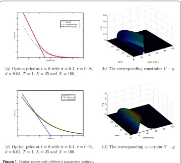
Figure 1Option prices with different parameter settings

4 Numerical experiments

In this section, we shall present some numerical results as well as useful discussions on the performance and convergence of the HODIE finite difference scheme. In particular, we shall concentrate on calculating the errors and the convergence rate of the current scheme through the following examples.

4.1 Computed option price and optimal exercise prices

Depicted in Fig.1(a) and Fig.1(c) are two sets of American put prices as a function of the underlying but with different parameter settings. From these figures, it is clear that the option price is a decreasing function of the underlying. Moreover, the “smooth pasting” conditions across the free boundary, which are usually difficult to implement numerically, are also satisfied well. One could observe from these two figures that the American option price dominates its European counterpart. This makes sense, as the right of being able to exercise earlier, in comparison to the European-style options, has added additional values to the option price. Besides the option prices, the differences between the option price, and the payoff, i.e.,V–g, are further shown in Fig.1(b) and Fig.1(d) for the two cases. From these two figures, it is observed that the option prices computed using our method are always greater than or equal to the payoff value at any time to maturity, which is one of the essential properties of American options.

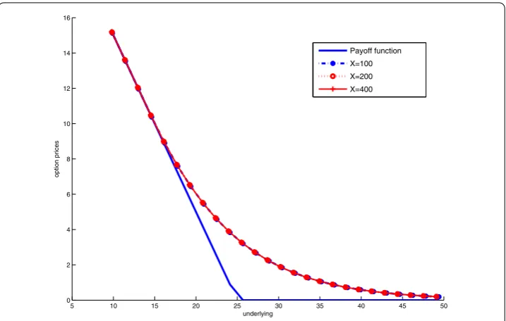
Figure 2Impacts of the truncation of the domain. Model parameters areσ= 0.3,r= 0.1,D= 0,

T–t= 1(year),E= $25

computed with otherwise identical but differentX, as displayed in Fig.2. One could clearly observe from this figure that the option prices with different choices ofXagree perfectly well with each other. Numerical calculation further shows that the maximum pointwise error among them is in the order of 10–4, which is indeed negligible from a financial point of view.

It is known that the optimal exercise price is far more difficult to determine accurately than the option price. From our algorithm described in Sect.3.1, it is clear that the opti-mal exercise price can be obtained as the maximum underlying at whichV_2,ij =gi–vj1,iis satisfied. Based on this fact, we calculate the optimal exercise prices withN= 2048 and K= 4096, and compare the numerical values with those calculated by the IFE method and Zhu’s analytical approach [48], as shown in Fig.3. From this figure, one can clearly observe that our numerical results agree well with those calculated using other methods. A close examination reveals that the current approach slightly underestimates theSf values when the time is close to expiry. This is not surprising because of the well-known singularity at expiry [18], which is not possible for most of the numerical schemes to deal with.

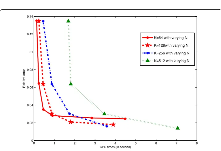
Another important issue in finance industry is the speed of calculation, which is equally important, sometimes even more, than the accuracy. To clearly demonstrate the overall numerical performance of the current approach, we display in Fig.4the relationship be-tween the efficiency and accuracy of our scheme. Here, the computational efficiency is measured by the total CPU time in seconds consumed for each run, whereas the accuracy is measured by the relative error over the whole computational domain, which is defined as

Relative error = V–Vexact ∞ Vexact ∞

Figure 3Comparison of the optimal exercise price. Model parameters areσ= 0.3,r= 0.1,D= 0,

T–t= 1(year),E= $100,X= 400

Figure 4CPU VS Accuracy. Model parameters areσ= 0.4,r= 0.06,D= 0.02,T–t= 1(year),E= $25,X= 100

with V andVexactdenoting the computed values and the reference values, respectively, and · ∞being the infinite norm. We remark that the approximate solution calculated on very

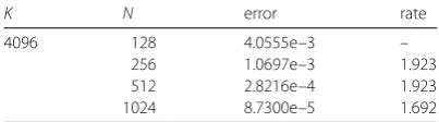
Table 1 Error estimate and convergence rate for the spatial direction with the same parameters as used in Fig.1(c)

K N error rate

4096 128 4.0555e–3 –

256 1.0697e–3 1.923

512 2.8216e–4 1.923

1024 8.7300e–5 1.692

From Fig.4, one can clearly observe that the efficiency of the current scheme is inversely varying with the accuracy. In other words, a demand in high accuracy in the computed op-tion price requires more computaop-tional time. However, by using our method, it is possible to produce a result with the relative error being less than 5%within 1 second. This level of accuracy and efficiency certainly suits the practical needs of financial market [51].

4.2 Convergence rate

As demonstrated in Sect.3.2, our method is first and second order convergent in the time and spatial directions, respectively. To further verify this theoretical result, we turn to in-vestigating the error estimate and convergence rate of the current method from a numeri-cal point of view. Since we do not have the exact solution of American options in hand, we shall adopt the approximate solution calculated on very fine grid sizes, i.e., withN= 2048 andK= 4096, as the exact solution. For comparison purpose, we use linear interpolation to get values at desired points, because “the exact solution” here is only known on mesh points.

To obtain the convergence rate along the spatial direction, we fix the size of the time step to be fairly small, i.e.,K= 4096, and vary the number of spatial intervals from 128 to 1024. The errors reported in Table1are measured by the discrete maximum norm defined as

eN,K=max

i,j V N,K

i,j –V¯(xi,tj).

With the errors associated with differentNavailable, the convergence rate along the spatial direction is then calculated from

RN,K=log₂

eN,K e2N,K

.

From Table1, one can clearly observe that _ee2NN,K,K is close to 4 for sufficiently largeK,

which indicates that our method is second order convergent in the spatial direction. This agrees with our theoretical convergence result stated in Theorem1.

Similarly, when we fix the spatial step size toN= 2048 and increase the grid number in the time direction, we find that the rate approaches 1, as shown in Table2. This indicates that a first order convergence is achieved in the time direction.

To better investigate the convergence rate of the current scheme, we also calculate the ratio with the time and spatial steps adjusted to each other according to the expected order of error O(h2_{+t). Specifically, we choose varying grid numbersN}

Table 2 Error estimate and convergence rate for the time direction with the same parameters as

Table 3 Global error estimate and convergence rate with the same parameters as used in Fig.1(c)

n error rate

1 4.24e–2 –

2 1.33e–2 1.67

4 4.20e–3 1.66

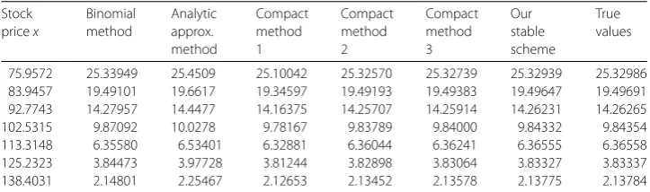
Table 4 Comparison of the American put option values at different underlying values with parameters:σ= 0.3,t= 0,T= 1,r= 0.04,d= 0.02,E= 100,X= 400

75.9572 25.33949 25.4509 25.10042 25.32570 25.32739 25.32939 25.32986 83.9457 19.49101 19.6617 19.34597 19.49193 19.49383 19.49647 19.49691 92.7743 14.27957 14.4477 14.16375 14.25707 14.25914 14.26231 14.26265

102.5315 9.87092 10.0278 9.78167 9.83789 9.84000 9.84332 9.84354

113.3148 6.35580 6.53401 6.32881 6.36044 6.36241 6.36555 6.36558

125.2323 3.84473 3.97728 3.81244 3.82898 3.83064 3.83327 3.83337

138.4031 2.14801 2.25467 2.12653 2.13452 2.13578 2.13775 2.13784

We also compare our scheme with binomial method, analytic approximation method proposed in [20], and compact finite difference methods proposed in [47], as shown in Table4. The values in this table are computed with the following parameter settings. The binomial method is based on time stept= 0.01, the analytical approximation method is based on time stept= 0.02, whereas compact finite difference methods 1, 2, and 3 are based on space steph= 0.02 and time stept= 0.0005. In our stable scheme, we use time step t= 0.0005 andN= 20,000 mesh points for spatial discretization which has almost the same number of mesh points as the compact methods. The true option values are based on the trinomial method proposed in [1] using time stept= 0.00005. From Table4, one can observe that our solution agrees perfectly well with the true option price, which indicates that our scheme is more accurate than other methods.

5 Conclusion

method also may be extended to price other kinds of American-style options, for exam-ple, American-style options in multi-dimensions, American-style options under a modi-fied Black–Scholes equation with fractional derivatives.

Acknowledgements

We would like to thank the anonymous reviewers for some suggestions for the improvement of this paper.

Funding

The work was supported by the Project of Philosophy and Social Science Research in Zhejiang Province (Grant No. 15NDJC243YB), National Natural Science Foundation (Grant No. 11201430) of China, Humanities and Social Sciences Planning Fund of Ministry of Education of China (Grant No. 18YJAZH002), Major Humanities and Social Sciences projects in colleges and universities of Zhejiang (Grant No. 2018GH020), Ningbo Municipal Natural Science Foundation (Grant Nos. 2017A610131, 2017A610140, 2015A610161), and Zhejiang Province Natural Science Foundation (Grant No.

LY18A010001). This research was also supported by the National Natural Science Foundation of China NO. 11601189, and Natural Science Foundation of Jiangsu Province NO. BK20160156.

Competing interests

The authors declare that they have no competing interests.

Authors’ contributions

The two authors have equal contributions. While the first author carried out the literature review, designed the numerical algorithm, and conducted numerical experiments, the second author participated in designing the algorithm and doing numerical experiments. The second author wrote the draft. All authors read and approved the final manuscript.

Author details

1_{Institute of Mathematics, Zhejiang Wanli University, Ningbo, P.R. China.}2_{Department of Business, School of Finance,}

Jiangnan University, Jiangsu, China.

Endnote

a _{An M-matrix is a Z-matrix with eigenvalues whose real parts are nonnegative. Here, the Z-matrix is a matrix with}

off-diagonal entries less than or equal to zero.

Publisher’s Note

Springer Nature remains neutral with regard to jurisdictional claims in published maps and institutional affiliations.

Received: 6 December 2017 Accepted: 4 December 2018

References

1. Ahn, J., Song, M.: Convergence of the trinomial tree method for pricing European and American options. Appl. Math. Comput.189(1), 575–582 (2007)

2. Allegretto, W., Lin, Y., Yang, H.: Finite element error estimates for a nonlocal problem in American option valuation. SIAM J. Numer. Anal.39(3), 834–857 (2001)

3. Angermann, L., Wang, S.: Convergence of a fitted finite volume method for the penalized Black–Scholes equation governing European and American option pricing. Numer. Math.106(1), 1–40 (2007)

4. Carr, P.: Randomization and the American put. Rev. Financ. Stud.11, 597–626 (1997)

5. Cen, Z., Le, A.: A robust finite difference scheme for pricing American put options with singularity-separating method. Numer. Algorithms53(4), 497–510 (2010)

6. Cen, Z., Le, A.: A robust and accurate finite difference method for a generalized Black–Scholes equation. J. Comput. Appl. Math.235(13), 3728–3733 (2011)

7. Chen, W., Wang, S.: A power penalty method for a 2D fractional partial differential linear complementarity problem governing two-asset American option pricing. Appl. Math. Comput.305, 174–187 (2017)

8. Cheng, X., Xue, L.: On the error estimate of finite difference method for the obstacle problem. Appl. Math. Comput. 183(1), 416–422 (2006)

9. Chiarella, C., EI-Hassan, N., Kucer, A.: Evaluation of American option prices in a path integral framework using Fourier–Hermite series expansions. J. Econ. Dyn. Control23(9–10), 1387–1424 (1999)

10. Chockalingam, A., Muthuraman, K.: An approximate moving boundary method for American option pricing. Eur. J. Oper. Res.240, 431–438 (2015)

11. Clavero, C., Gracia, J.L.: A high order HODIE finite difference scheme for 1D parabolic singular perturbed reaction-diffusion problems. Appl. Math. Comput.218, 5067–5080 (2012)

12. Clavero, C., Gracia, J.L., Jorge, J.C.: High-order numerical methods for one-dimensional parabolic singularly perturbed problems with regular layers. Numer. Methods Partial Differ. Equ.21(1), 149–169 (2005)

13. Clavero, C., Gracia, J.L., Jorge, J.C.: A uniformly convergent alternating direction HODIE finite difference scheme for 2D time-dependent convection-diffusion problems. IMA J. Numer. Anal.26(1), 155–172 (2006)

14. Clavero, C., Gracia, J.L., Lisbona, F.: High order methods on Shishkin meshes for singular perturbation problems of convection-diffusion type. Numer. Algorithms22(1), 73–97 (1999)

15. Company, R., Egorova, V.N., Jódar, L.: Constructing positive reliable numerical solution for American call options: a new front-fixing approach. J. Comput. Appl. Math.291, 422–431 (2016)

17. Cox, J.C., Ross, S., Rubinstein, M.: Option pricing: a simplified approach. J. Financ. Econ.7(3), 229–264 (1979) 18. Evans, J.D., Kuske, R., Keller, J.B.: American options on assets with dividends near expiry. Math. Finance12, 219–237

(2002)

19. García, D.: Convergence and biases of Monte Carlo estimates of American option prices using a parametric exercise rule. J. Econ. Dyn. Control27, 1855–1879 (2002)

20. Geske, R., Johnson, H.E.: The American put option valued analytically. J. Finance39, 1511–1524 (1984)

21. Glowinski, R., Lions, J.L., Trémolières, T.: Numerical Analysis of Variational Inequality. North-Holland, Amsterdam (1984) 22. Goeleven, D.: A uniqueness theorem for the generalized-order linear complementarity problem associated with

M-matrices. Linear Algebra Appl.235, 221–227 (1996)

23. Hajipour, M., Jajarmi, A., Baleanu, D.: An efficient non-standard finite difference scheme for a class of fractional chaotic systems. J. Comput. Nonlinear Dyn.13(2), 021013 (2017)

24. Hajipour, M., Jajarmi, A., Malek, A., Baleanu, D.: Positivity-preserving sixth-order implicit finite difference weighted essentially non-oscillatory scheme for the nonlinear heat equation. Appl. Math. Comput.325, 146–158 (2018) 25. Hon, Y.C., Mao, X.Z.: A radial basis function method for solving options pricing model. J. Financ. Eng.8, 31–49 (1997) 26. Huang, J., Pang, J.S.: Option pricing and linear complementarity. J. Comput. Finance2(1), 31–60 (1998)

27. Jajarmi, A., Hajipour, A.: Efficient finite difference method for the time-delay optimal control problems with time-varying delay. Asian J. Control19(2), 554–563 (2017)

28. Jajarmi, A., Hajipour, M., Baleanu, D.: New aspects of the adaptive synchronization and hyperchaos suppression of a financial model. Chaos Solitons Fractals99, 285–296 (2017)

29. Kalantari, R., Shahmorad, S., Ahmadian, D.: The stability analysis of predictor-corrector method in solving American option pricing model. Comput. Econ.47(2), 255–274 (2016)

30. Kangro, R., Nicolaides, R.: Far field boundary conditions for Black–Scholes equations. SIAM J. Numer. Anal.38(4), 1357–1368 (2000)

31. Kellogg, R.B., Tsan, A.: Analysis of some difference approximations for a singular perturbation problem without turning points. Math. Comput.32(144), 1025–1039 (1978)

32. Khaliq, A.Q.M., Voss, D.A., Kazmi, K.: Adaptiveθ-methods for pricing American options. J. Comput. Appl. Math.222(1), 210–227 (2008)

33. Longstaff, F.A., Schwartz, E.S.: Valuing American options by simulation: a simple least-squares approach. Rev. Financ. Stud.14(1), 113–147 (2001)

34. Momani, S., Rqayiq, A.A., Baleanu, D.: A nonstandard finite difference scheme for two-sided space-fractional partial differential equations. Int. J. Bifurc. Chaos22(04), 1250079 (2012)

35. Muthuraman, K.: A moving boundary approach to American option pricing. J. Econ. Dyn. Control32(11), 3520–3537 (2008)

36. Rad, J.A., Parand, K., Ballestra, L.V.: Pricing European and American options by radial basis point interpolation. Appl. Math. Comput.251, 363–377 (2015)

37. Shi, X.-J., Yang, L., Huang, Z.-H.: A fixed point method for the linear complementarity problem arising from American option pricing. Acta Math. Appl. Sin.32(4), 921–932 (2016)

38. Sweilam, N.H., Rizk, M.M., Abou Hasan, M.M.: Non-uniform finite difference method for European and American put option. J. Fract. Calc. Appl.3S(5), 1–11 (2014)

39. Tangman, D.Y., Gopaul, A., Bhuruth, M.: Numerical pricing of options using high-order compact finite difference schemes. J. Comput. Appl. Math.218(2), 270–280 (2008)

40. Tangman, D.Y., Gopaul, A., Bhuruth, M.: A fast high-order finite difference algorithm for pricing American options. J. Comput. Appl. Math.222(1), 17–29 (2008)

41. Wang, S., Yang, X.Q., Teo, K.L.: Power penalty method for a linear complementarity problem arising from American option valuation. J. Optim. Theory Appl.129(2), 227–254 (2006)

42. Wilmott, P., Dewynne, J., Howison, S.: Option Pricing: Mathematical Models and Computation. Oxford Financial Press, Oxford (1993)

43. Wu, L., Kwok, Y.K.: A front-fixing finite difference method for the valuation of American options. J. Financ. Eng.6(2), 83–97 (1997)

44. Yaseen, M., Abbas, M., Nazir, T., Baleanu, D.: A finite difference scheme based on cubic trigonometric b-splines for a time fractional diffusion-wave equation. Adv. Differ. Equ.2017(1), 274 (2017)

45. Zhang, K., Song, H., Li, J.: Front-fixing FEMs for the pricing of American options based on a PML technique. Appl. Anal. 94(5), 903–931 (2015)

46. Zhang, K., Wang, S., Yang, X.Q., Teo, K.L.: A power penalty approach to numerical solutions of two-asset American options. Numer. Math., Theory Methods Appl.2(2), 202–223 (2009)

47. Zhao, J., Davison, M., Corless, R.M.: Compact finite difference method for American option pricing. J. Comput. Appl. Math.206(1), 306–321 (2007)

48. Zhu, S.-P.: An exact and explicit solution for the valuation of American put options. Quant. Finance6(3), 229–242 (2006)

49. Zhu, S.-P.: A new analytical-approximation formula for the optimal exercise boundary of American put options. Int. J. Theor. Appl. Finance9(7), 1141–1177 (2006)

50. Zhu, S.-P., Chen, W.-T.: A predictor-corrector scheme based on the ADI method for pricing American puts with stochastic volatility. Comput. Math. Appl.62(1), 1–26 (2011)

51. Zhu, S.-P., Chen, W.-T.: An inverse finite element for pricing of American options. J. Econ. Dyn. Control37(1), 231–250 (2013)

52. Zhu, S.-P., He, X.-J., Lu, X.: A new integral equation formulation for American put options. Quantitative Finance (2017, in press)

53. Zhu, S.-P., Zhang, J.: A new predictor-corrector scheme for valuing American puts. Appl. Math. Comput.217(9), 4439–4452 (2011)

54. Zhu, Y., Chen, B., Ren, H., Xu, H.: Application of the singularity-separating method to American exotic option pricing. Adv. Comput. Math.19, 147–158 (2003)