Bayesian LASSO for Quantitative Trait Loci Mapping

DOI: 10.1534/genetics.107.085589

Bayesian LASSO for Quantitative Trait Loci Mapping

Nengjun Yi*

,1

_{and Shizhong Xu}

†

*Department of Biostatistics, Section on Statistical Genetics, University of Alabama, Birmingham, Alabama 35294 and†Department of Botany and Plant Sciences, University of California, Riverside, California 92521

Manuscript received December 10, 2007 Accepted for publication March 14, 2008

ABSTRACT

The mapping of quantitative trait loci (QTL) is to identify molecular markers or genomic loci that influence the variation of complex traits. The problem is complicated by the facts that QTL data usually contain a large number of markers across the entire genome and most of them have little or no effect on the phenotype. In this article, we propose several Bayesian hierarchical models for mapping multiple QTL that simultaneously fit and estimate all possible genetic effects associated with all markers. The proposed models use prior distributions for the genetic effects that are scale mixtures of normal distributions with mean zero and variances distributed to give each effect a high probability of being near zero. We consider two types of priors for the variances, exponential and scaled inverse-x2 _{distributions, which result in a} Bayesian version of the popular least absolute shrinkage and selection operator (LASSO) model and the well-known Student’st model, respectively. Unlike most applications where fixed values are preset for hyperparameters in the priors, we treat all hyperparameters as unknowns and estimate them along with other parameters. Markov chain Monte Carlo (MCMC) algorithms are developed to simulate the param-eters from the posteriors. The methods are illustrated using well-known barley data.

Q

UANTITATIVE traits are controlled by multiple quantitative trait loci (QTL). The genetic ef-fects of QTL and the phenotypic value of a quantitative trait are usually described by a linear model. Since the locations of QTL are not knowna priori, we often use markers to represent QTL. Some markers may be closely linked to one or more QTL, and thus they may show strong association with the trait. Most markers, how-ever, may not be directly linked to QTL, and thus no association will be expected between these markers and the trait. Interval mapping or the equivalent single-marker analysis does not provide accurate estimates of QTL effects because the single-QTL model used by the method is seldom the correct model. The multiple-QTL model is the reasonable choice for mapping quantitative traits (Kao et al.1999).

When all markers are included in the QTL analysis, the model may be oversaturated. Variable selection may be conducted to include and exclude markers in the model (Sillanpa¨ a¨and Arjas1998; Yiet al.2003, 2005;

Yi2004; Yiand Shriner2008). An alternative approach

is a shrinkage method that includes all variables in the model and uses informative prior distributions to shrink trivial effects toward zero. Ridge regression (Hoerland

Kennard1970) is a shrinkage procedure and can be

obtained using independent and identical normal

priors centered at zero, with the degree of shrinkage controlled by the prior variance. The least absolute shrinkage and selection operator (LASSO) is another shrinkage method that has been widely used in re-gression analysis for large models (Tibshirani1996). It

minimizes the residual sum of squares constraining the sum of absolute values of the regression coefficients, t$ Pjb_jjfort$0, if the response and the predictors are standardized. This special constraint allows some estimated regression coefficients to be exactly zero. This selective or individualized shrinkage allows LASSO to handle extremely large models. Mathematically, the LASSO estimates of regression coefficients can be achieved by

min

b;l

yXXjbj T

yXXjbj

1lXjb_jj

h i

;

where l $0 is a Lagrange multiplier, which relates implicitly to the bound t and controls the degree of shrinkage. The LASSO estimates of coefficients can be efficiently computed via the LARS algorithm of Efron

et al.(2004). The LASSO procedure can be interpreted as a Bayesian posterior mode estimate when assigning an independent double-exponential prior to each b_j (e.g., Tibshirani1996; Yuanand Lin2005; Parkand

Casella 2007). Recently, Xu (2007) successfully

ap-plied the LASSO method to estimate the epistatic effects of QTL. However, the LASSO provides no estimate for the residual error variance and no interval estimate for a 1_{Corresponding author:Department of Biostatistics, University of Alabama,}

Birmingham, AL 35294-0022. E-mail: [email protected]

regression coefficient and needs to predetermine the parameterl(Tibshirani1996; Efron_{et al.}2004).

There are some other shrinkage methods that have been applied to mapping multiple QTL. The method of Xu (2003) simultaneously fits maker effects of the

entire genome in a regression model and assigns each effect a normal prior with mean 0 and an effect-specific variance (also see Wanget al.2005; Hotiand Sillanpa¨ a¨

2006; Huanget al.2007). The variance parameters are

further assigned the noninformative Jeffrey’s prior, which in turn induces improper priors on the coeffi-cients. Meuwissen et al. (2001) and Xu (2007) used

scaled inverse-x2 _{distributions with predetermined}

hy-perparameters as priors for the effect-specific variance parameters. Rather than presetting the hyperparameters in the priors that control the degree of shrinkage, it would be appealing to treat the hyperparameters as unknowns and estimate them from the data so that the model can shrink the coefficients as much as can be justified by the data. Parkand Casella(2007) set up a

hyperprior for the hyperparameter in the LASSO model and developed a Gibbs sampler to fit the hierarchical model. R. B. O’Haraand M. J. Sillanpa¨ a¨(unpublished

results) conducted a comparison with several Bayesian model selection and shrinkage methods, including Bayesian LASSO and the method of Xu(2003).

In this article, we propose several Bayesian hierarchi-cal models for mapping multiple QTL that simulta-neously fit and estimate all possible genetic effects associated with all markers across the entire genome. We use prior distributions for the genetic effects that are scale mixtures of normal distributions with mean zero and unknown effect-specific variances. We con-sider two types of priors for the variances, exponential and scaled inverse-x2 _{distributions, which result in a}

Bayesian version of the LASSO model and the well-known Student’s t model, respectively. We treat all hyperparameters as unknowns and estimate them along with other parameters. We fit the models in a fully Bayesian approach, employing the Markov chain Monte Carlo (MCMC) simulation to generate posterior samples from the joint posterior distribution. Our methods give not only point estimates but also interval estimates of all parameters and provide natural means of assessing model uncertainty.

MULTIPLE-QTL MODEL

We describe our method primarily for a mapping population with only two segregating genotypes,e.g., a backcross, double-haploid (DH), or recombinant in-bred line (RIL). The method can be extended to other types of population. Assume that we observe many markers across the genome. The aim of QTL mapping is to identify which markers are tightly linked to genes with detectable effects and to estimate the magnitudes of the effects. For a continuously distributed trait, the

observed phenotypic value yi of individual i can be

described by the linear regression model

yi¼m1 Xp

j¼1

xijbj1eibm1Xib1ei; i¼1;2; ;n;

ð1Þ

wherepis the number of markers,mis the overall mean, xijdenotes the genotype of markerjfor individualiand

is defined as0.5 and 0.5 for the two genotypes in the mapping population, the coefficientb_j represents the main effect of markerj,eiis the residual error assumed

to follow aNð0;s2_{Þdistribution,X}

i ¼ ðxi1; ;xipÞ, and

b¼ ðb₁; ;b_pÞT.

In practice, some marker genotypes may be missing. There are two commonly used methods to deal with missing marker data. The first approach takes the uncertainty in missing genotypes into account by treat-ing the misstreat-ing genotypes as unknowns and sampltreat-ing them in the MCMC update procedure. The second approach is similar to the regression model of Haley

and Knott(1992) and replaces all missing genotypes by

their expected values conditioning on the observed marker data, using the multipoint method (Jiangand

Zeng1997). Although the second method ignores the

uncertainty of the estimated marker genotypes, it has a big computational advantage over the first method. Both approaches can be incorporated into our Bayesian method. For simplicity and computational conve-nience, this study considers only the second method.

PRIOR DISTRIBUTIONS

Data are usually sufficient to estimate the overall meanmand the residual variances2_{. Thus, we can use}

any reasonable noninformative prior distributions for these parameters. For example, we can use an indepen-dent, flat prior form,i.e.,pðmÞ 1, and a noninforma-tive scale-invariant prior 1/s2_fors2_.

QTL data typically contain a large number of markers, leading to many coefficients in model (1). However, most of the coefficients are expected to have no or only weak effects on the phenotype. Only a few coefficients may have notable effects (see, e.g., Xu

2003). To incorporate this prior knowledge into our analysis, therefore, we set up a prior distribution that gives each coefficientb_ja high probability of being near zero and in the meantime gives each coefficient a chance to take a large effect.

A commonly used prior that has the above properties is the double exponential (also called Laplace) distribution

pðbÞ ¼Y

p

j¼1

l 2e

ljb_jj _ð2Þ

(Tibshirani1996; Parkand Casella2007), wherelis

the posterior mode estimate of the coefficientsbis the LASSO estimate (Tibshirani1996; Parkand Casella

2007). Another wide-tailed distribution is the well-known Student’stdistribution,

pðbÞ ¼Y

p

j¼1

tnðb_jja;s2Þ; ð3Þ

where the hyperparametersn,a, ands2_{are the degrees}

of freedom, the location, and the scale parameters, respectively (see, e.g., Sorensen and Gianola 2002;

Gelmanet al.2003; Varonaet al.2005).

Both the double-exponential distribution and Stu-dent’s t distribution can be presented as a two-level hierarchical model (see, e.g., Andrews and Mallows

1974; Griffinand Brown2006). Compared with their

original forms, the two-level hierarchical models are easier to deal with both analytically and computationally. In the two-level hierarchical models, the first level assumes that the coefficients b_j follow independent normal distributions with mean zero and unknown variancest2

j,

bjt2 Y

p

j¼1

Nðb_jj0;t2_jÞ; ð4Þ

wheret2_{¼ ðt}2 1; ;t

2

pÞ. At the second level, we assume

that the variancest2

j follow some specified independent

prior distributions

t2juY

p

j¼1

pðt2_jjuÞ; ð5Þ

where u includes all the hyperparameters. The above two-level priors result in a scale mixture of normal distributions for the coefficientsb_j,

bpðbjuÞ ¼Y

p

j¼1

ð‘

0

Nðb_jj0;t2_jÞpðt2_j juÞdt2_j; ð6Þ

wherepðt2

jjuÞis referred to as the mixing distribution.

From this, we see that two-level hierarchical models introduce different variance parameters for different coefficients and hence induce different amounts of shrinkage in the estimates of different coefficients. The variance components are not the parameters of interest, but they are useful intermediate quantities to facilitate better inferences for the individual regression coeffi-cients (e.g., Gelman2005).

The double-exponential distribution (2) can be presented as a mixture of normal distributions (4) with the mixing distributionpðt2

jjuÞbeing an exponential

distribution Expon(l2_{=2) or equivalently a gamma}

distribution Gamma(1,l2_=2),

p t2

j jl

¼Expon t2 j j l2 2 ¼l 2 2 e l2_t2

j=2_{; ð7Þ}

wherel2_{=2 is the inverse scale that needs to be carefully}

preset or estimated from the data.

For any values of l, the mode of the exponential distribution Expon(l2_{=2)¼0, meaning that the ‘‘most}

likely’’ values oft2

j and thusbj are zero. However, the

variance oft2

j is 4=l

4_{, strongly depending on the value}

ofl. Instead of presetting a value forl, it is appealing to assign a prior distribution to l also so that l can be estimated along with other parameters. This pro-cedure obviates the choice of l and automatically accounts for the uncertainty in its selection that affects the estimates of regression coefficients (Park and

Casella 2007). For convenience, we regard l2=2,

instead of l, as the parameter of interest. Following Park and Casella (2007), we assign a conjugate

gamma prior Gamma(a, b), a . 0, b . 0, to the parameterl2_{=2. Assigning a prior distribution tol}2₌₂

provides a way to estimatel2_{=2. We setaandbas small}

values (e.g.,a¼0.1 andb¼0.1) so that the prior for l2_{=2 is essentially noninformative.}

Student’s t distribution (3) can be expressed as a mixture of normal distributions (4) with the mixing distributionpðt2

j juÞbeing a conjugate scaled inverse-x

2

distribution Inv-x2_ðn;s2_{Þor equivalently an inverse gamma}

distribution Inv-gamma(n=2,ðn=2Þs2_),

pðt2_j jn;s2Þ ¼Inv-x2_ðt2

jjn; s2Þ}ðt2jÞ

ðn=211Þ_{exp n} s2= 2t2

j

;

ð8Þ

where the hyperparameters n.0 ands2_{.0 represent}

the degrees of freedom and the scale of the distribution, respectively.

The amount of shrinkage in the prior (8) depends on the values of the hyperparameters n and s2_{. The}

improper distribution pðt2

jÞ}t

2

j , which is equivalent

to the uniform distribution on logt2

j, has the form of

the inverse-x2_{density withn¼0 ands}2 _{¼0 and can be}

taken as a limit of the proper inverse-x2 _or

inverse-gamma densities. This improper prior in turn induces an improper prior for b_j of the form pðb_jÞ}jb_jj1 (Griffinand Brown 2006). In the class of inverse-x2

densities, Inv-x2_{ð0;0Þhas the constant degree of}

shrink-age in the coefficient estimates. Xu(2003) actually used

this improper prior pðt2

jÞ}t

2

j in his shrinkage QTL

mapping.

We here treatn ands2 _{as unknown parameters,}

ob-viating the choice of (n,s2_{) and automatically}

account-ing for the uncertainty in its selection that affects the estimates of the regression coefficients. We assign a uni-form density on 1/nfor the range (0, 1] and a uniform distribution onsfor the range (0,AwithAbeing a large number (see Gelmanet al.2003).

pro-posed an alternative version of the prior onb_j that is dependent on the residual variances2_,

bjt2 Y

p

j¼1

Nb_jj0;s2t2_j; ð9Þ

where t2_{¼ ðt}2

1; ;t2pÞ. At the second level, the prior

distributions ont2

j take the same form as (7) or (8). This

conditional prior may have some advantages; for exam-ple, it results in thatlis unitless and posteriors induced from (9) generally do not have more than one mode (Parkand Casella2007).

We now have introduced two different priors for b_j and two different priors fort2

j. The two priors forbjare

p1ðbjÞ ¼Nðbjj0;t2jÞ and p2ðbjÞ ¼Nðbjj0;s2t2jÞ,

re-spectively. The two priors for t2

j are p1ðt2jÞ ¼

Exponðt2

jjl

2_{=2Þ and p}

2ðt2jÞ ¼Inv-x

2_ðt2

j jn;s

2_Þ,

respec-tively. This yields four possible combinations and thus four different models. These four models are called model I with prior p₁ðb_jÞp₁ðt2

jÞ, model II with prior

p2ðbjÞp1ðt2_jÞ, model III with prior p1ðbjÞp2ðt2_jÞ, and

model IV with priorp2ðbjÞp2ðt2jÞ.

POSTERIOR COMPUTATION

We fit the models using the MCMC algorithm, applied to the joint posterior distribution of all the parameters ðm;b; s2_;t2_{;uÞ. The joint posterior distribution can be}

expressed as

pðm;b;s2_;t2_;ujyÞ

}Y

n

i¼1

pðyijm;b;s2ÞpðmÞpðs2Þ

Yp

j¼1

p b _jjt2_jp t _j2jupðuÞ;

ð10Þ

wherey¼ ðy1; ;ynÞT,b¼ ðb1; ;bpÞ T

,t2 _{¼ ðt}2 1; ;

t2

pÞ, urepresents lfor models I and II and (n;s

2_{) for}

models III and IV,pðyijm;b;s2Þis the normal density

functionNðm1Xib;s2Þ, and other terms in the

right-hand side are the priors defined in the last section. For notational convenience, we suppress the dependence onXhere and afterward.

With the two-level hierarchical models as set up in the last section, the joint posterior distributionpðm;b;s2_;

t2_{;ujyÞcan be simulated using the MCMC algorithm,}

alternately updating m from the normal distribution pðmjy;b;s2_{Þ, updating each b}

j from the normal

dis-tribution pðb_jjy;m;b_j;s2_{; t}2_{Þ, where b}

j represents

all elements ofbexceptb_j, updatings2_{from the}

inverse-x2_{distributionpðs}2_{jy;m;bÞ, updating eacht}2

j from the

inverse Gaussian (for models I and II) or inverse-x2

dis-tribution (for models III and IV), and updatingl2_{=2 from}

the gamma distributionpðl2_jt2_{Þ(for models I and II), or}

updatings2_{from the gamma distributionpðs}2_jt2_;nÞand

updatingnfrompðnjy;m;b;s2_;t2_{Þ, using a Metropolis}

step (for models III and IV).

The two-level hierarchical modeling allows us to easily derive the above conditional posterior distributions (see appendix a). For all the four proposed models,

however, the above MCMC algorithms can be per-formed directly using the Bayesian software WinBUGS14 (Spiegelhalteret al.2002), and thus we actually do not

need to derive the conditional posteriors. However, the expressions of the conditional posteriors allow us to develop faster, purpose-built programs. The WinBUGS code implementing these four hierarchical models can be obtained by request from the first author.

The MCMC algorithm proceeds to draw each un-known from its fully conditional posterior distribution, given the current values of all other unknowns and the observed data. Each iteration of the MCMC algorithm cycles through all elements ofðm; b;s2_;t2_{;uÞ. This}

pro-cess continues for a large number of iterations to obtain random samples from the joint posterior distribution. We run multiple parallel chains with overdispersed starting points and use the potential scale reduction factor Rˆ that compares the between- and within-se-quence variances for any scalar estimands, to monitor convergence (Gelmanet al.2003). We use the condition

of Rˆ , 1.1 for all scalar estimands of interest as the criteria of convergence. Once our simulations have converged, we continue to draw thousands of simula-tions and treat them as a sample from the joint posterior distribution. We thin the sequences by keeping every kth simulation draw from each sequence and discarding the rest (e.g.,k¼100).

POSTERIOR SUMMARY AND INTERPRETATION

The proposed Bayesian hierarchical models can pro-vide various graphical and tabular summaries that assess the contribution of individual loci while adjusting for effects of all other possible loci. One of such summaries is the estimate of the genetic effectsb_j associated with each marker. Furthermore, using the posterior samples ofb_j and the observed valuesxij, we can also calculate

the proportion of the phenotypic variance explained by each effect (i.e., heritability),h2

j ¼Vjb2j=Vy, whereVyis

the phenotypic variance andVjis the sample variance of

fxij;i¼1; ;ng. The heritabilityh2j is independent of

the scale of the phenotype, while the effect size b_j depends on it. The fully Bayesian analysis usually uses the posterior median or mean to estimateb_jandh2

j and

also can provide the posterior interval for the estimate. The Bayesian hierarchical models shrink the ‘‘in-significant’’ coefficients to zero, and hence the posterior estimates of b_j and h2

j can guide variable selection.

However, these posterior summaries do not automati-cally provide a criterion to declare that an effect is ‘‘in’’ the model. Hotiand Sillanpa¨ a¨(2006) suggest setting

effects in Hoti and Sillanpa¨ a¨ (2006). Yangand Xu

(2007) proposed using a Wald test statistic.

We here construct an alternative measurement that is similar to the widely used LOD score in the traditional QTL mapping approach if the phenotype is affected by a single QTL (Lander and Botstein1989), following

the idea of Yandellet al.(2007) (also see the vignette in

the package R/qtlbim). We call this statistic the approx-imate Bayesian LOD score. The approxapprox-imate Bayesian LOD score can be conveniently compared with the LOD curve obtained from the traditional interval-mapping approach. Our Bayesian LOD score considers the contribution of a given locus to the LOD after adjusting effects for all other possible loci. For marker j, the Bayesian LOD score (BLOD) is calculated as

BLODj¼2 log10

Qn

i¼1Nðyijm1Xib;s2Þ

Qn

i¼1N yijm1Xibxijbj;s2j

0 @

1 A;

ð11Þ

where the values ofm,b, ands2_{are the simulated draws}

in a certain iteration, and s2

j ¼ ð1=ðn2ÞÞ

Pn i¼1ðyi

mXib1xijbjÞ

2

, the mean of the conditional posterior pðs2_jy;m;b

jÞ ¼Inv-x2 n;ð1=nÞ

Pn

i¼1ðyimXib1

xijbjÞ

2_{Þ. Note that although we adjust for the residual}

error variance, we use the simulated draws under the full model (including xijbj) to calculate the likelihood

function for the reduced model (withoutxijbj).

REAL DATA ANALYSIS

The well-known barley data set from the North Amer-ican Barley Genome Mapping Project (Tinkeret al.1996)

was analyzed using the four proposed Bayesian hierarchi-cal models. This data set has been extensively analyzed

using different methods (Tinkeret al.1996; Xu2003,

2007; Yiet al.2003, 2005; Zhanget al.2005; Xuand Jia

2007). The data were collected from a doubled-haploid population that containedn¼145 lines; each was grown in 25 different environments. The phenotype analyzed was the average value of kernel weight across environ-ments. A total of p¼127 mapped markers covering a genome of 1500 cM (seven chromosomes) were used in the analysis. Observed marker genotypes were coded as

0.5 for one genotype and10.5 for the other genotype.

The data contain5% missing marker genotypes. The missing marker genotypes were replaced by their ex-pected values conditioning on the observed marker data using the multipoint method. We simultaneously mod-eled all 127 marker effects in the linear regression (1). For all four proposed models, the MCMC simula-tions were performed in the Bayesian software Win-BUGS14 (Spiegelhalteret al.2002), linked from the

R statistical computing software (Sturtz et al. 2005;

R DevelopmentCoreTeam2006), which we can use to

conveniently plot the results. For each analysis, we ran three parallel simulation sequences with starting points randomly generated from the prior distributions. The models with the dependent prior (9) (models III and IV) were found to converge slightly quicker than those with the independent prior (4) (models I and II). For all four models, the potential scale reduction factor Rˆ values fell below 1.1 for all parameters after5000 iter-ations, indicating that the chains converged adequately (data not shown). For each of the three parallel se-quences, therefore, we ran a total of 20,000 iterations and discarded the first halves to allow adequate conver-gence. The remaining 10,000 posterior samples of each sequence were thinned to 1000 for estimating the posterior distribution of quantities of interest by keep-ing every 10th simulation draw from each sequence and

Figure 1.—Posterior medians (points) and

discarding the rest. On a dual processor 2.4-GHz ma-chine, each analysis took4.5 hr.

To investigate whether or not posterior inferences are affected by the values of the shape a and the inverse scalebin the gamma prior Gamma(a,b), we analyzed models I and II with four different values of (a,b),a¼ b¼0.01, 0.1, 0.5, 1. Under the four analyses, the posterior

estimates of the parametersðm;b;s2_;t2_{Þwere identical,}

but the inverse scalel2_{=2 differed slightly.}

Figure 1 shows the posterior medians and the 95% posterior intervals for the marker effects b_j and the proportion of the phenotypic variance explained by each effect (i.e., heritability) h2

j. Models I and II

pro-duced almost identical results, both being able to identify markers with large effects. The analyses showed four chromosomes (7, 1, 3, and 2) with strong evidence of QTL. The QTL on chromosome 3 was found to have an opposite effect on the phenotype to the other detected QTL and was missed in the analysis of Xu

(2003), who used the improper priorpðt2

jÞ}t

2

j . The

difference may also be caused by the different ways of treating missing marker genotypes for the two methods. As can be seen in Figure 1, the plots of the heritability can provide a clearer picture than those of the effect.

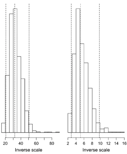
Figure 2 shows the histograms of the inverse scale l2_{=2 for the analyses of models I and II witha¼b¼0.1.}

We can see that the hyperparameter l2_{=2 can be}

estimated with quite high precision. For model I, the inverse scale parameter was estimated at 32.0, with a 95% posterior interval of½20.6, 50.5. However, model II provided a much smaller estimate, with a posterior median of 5.1 and a 95% posterior interval of½2.8, 9.8. We know that in the exponential distribution a larger inverse scale forces stronger shrinkage. Figure 1 shows that models I and II perform at the same level of shrinkage in the coefficient estimates. This can also be shown by looking at the estimateds2_{, which was 0.3,,1.}

Figure 3 depicts the posterior medians and the 95% posterior intervals for marker effectb_j and the herita-bilityh2

j from the analyses of models III and IV. Models

III and IV produced identical results, similar to those from models I and II. However, the Inv-x2 _prior

distri-butions on t2

j produced slightly larger posterior

me-Figure2.—Histogram of the posterior samples for the

in-verse scale of the exponential prior on the variances. The dot-ted lines represent the posterior 5, 50, and 95% quantiles. The left and right plots show inferences for models I and II, respectively.

Figure 3.—Posterior medians (points) and

dians and wider posterior intervals forb_j andh2

j. The

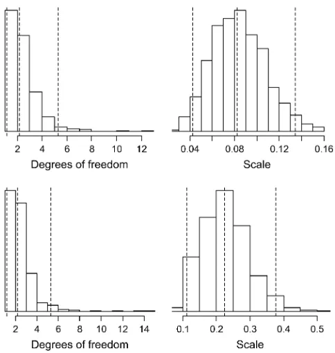
degrees of freedom and scale parameters can be esti-mated from the data. Figure 4 shows the histograms of these two hyperparameters for the analyses of models III and IV. The two models produced similar estimates for the degrees of freedom, with the posterior median at 2.1

and the 95% posterior interval of½1.2, 5.3. However, the estimate of the scale parameter for model IV was three times as large as that for model III.

Figure 5 (top) shows the posterior medians and the 95% posterior intervals for the Bayesian LOD score for model I. The other three models produced similar estimates (data not shown). For comparison, Figure 5 (bottom) also shows the LOD score curve calculated by the traditional interval mapping based on a single-QTL model. If we use the standard threshold value of 3.2, the interval mapping identified only two regions (on chromosomes 7 and 1, respectively), which have larger effects in our analyses. Our Bayesian models produced much higher estimates of LOD score and detected more significant QTL.

In the proposed two-level hierarchical models, the amount of shrinkage in the coefficient estimates is largely determined by the hyperparameters in the priors. It is expected that optimal values of the hyper-parameters depend on the data and the number of variables included, which makes it difficult to preset their values. To illustrate this, we analyzed the data with only markers on chromosomes 1, 3, and 7 included in the model. Figure 6 displays the plots of marker effects, showing that we were still able to detect the same QTL as in our previous analyses. As shown in Figure 7, however, the posterior estimates of the hyperparameters were different from those in the previous analyses.

DISCUSSION

We have presented four Bayesian hierarchical models that can be used to simultaneously fit and estimate all

Figure4.—Histogram of the posterior samples for the

de-grees of freedom and scale of the Inv-x2 _{prior on variances.} The dotted lines represent the posterior 5, 50, and 95% quan-tiles. The top and bottom plots show inferences for models III and IV, respectively.

Figure5.—The top plot shows posterior

possible genetic effects associated with all molecular markers across the entire genome. We found that these four methods perform equally well. It is knowna priori that most markers have no or little effect on the phe-notype, but if a marker has an effect, it could be large. To incorporate this prior knowledge into our analysis, we set up a continuous form of prior distribution for ge-netic effects that gives each effect a high probability of being near zero and also enables us to accommodate large effects. We have considered two such priors—double exponential distribution and Student’s t distribution—

that can be expressed as scale mixtures of normal distributions with mean zero and unknown variances distributed as exponential and scaled inverse-x2

distri-butions, respectively. The former prior results in a Bayesian LASSO model (Tibshirani 1996; Yuan and

Lin 2005; Park and Casella 2007), and the latter

includes Jeffrey’s noninformative prior as a special case (Gelman2006).

Both the exponential and the scaled inverse-x2

dis-tributions include hyperparameters that determine the degrees of shrinkage in the estimates of the variances

Figure 6.—Posterior medians (points) and

95% intervals (shaded lines) for genetic effects from all four models using markers on chromo-somes 1, 3, and 7. Inner tick marks on thex-axis represent the marker positions.

Figure7.—Histogram of the posterior samples

and thus the genetic effects. A common practice is to preset values for the hyperparameters using methods like cross validation (Tibshirani1996; Meuwissenet al.

2001; Xu 2003; Bao and Mallick 2004; Xu 2007).

However, optimal values depend on the data and thus may be difficult to choose. A novel aspect of our ap-proach is to treat all hyperparameters as unknowns and estimate them along with other parameters. This pro-cedure allows us to control the amount of shrinkage by taking advantage of the characteristics of the data. In contrast, Jeffrey’s prior includes no hyperparameter but always forces a constant degree of shrinkage. Xu(2003)

showed that Jeffrey’s prior yields good performance, but we observed that it converges more slowly than our proposed methods.

We fit the models in a fully Bayesian approach, employing the MCMC simulation to generate posterior samples from the joint posterior distribution, which can be used to make various posterior inferences. Although computationally intensive, it is easy to implement and provides not only point estimates but also interval estimates of all parameters. We have proposed graphical tools to summarize the posterior samples, notably the approximate Bayesian LOD score that can be easily compared with the results from traditional interval mapping. However, we realize that these tools still are informal and descriptive, due to the lack of formal threshold value to select markers. A formal choice of threshold value will be a topic of future research.

The fully Bayesian approach enables us to obtain much richer inferences about the models than most non-Bayesian analyses. In practice, however, it is desir-able to have a quicker calculation that merely looks for posterior modes rather than fully investigating the posterior distribution. The original LASSO estimates for linear regression coefficients are equivalent to Bayes-ian posterior mode estimates when the coefficients have independent and identical double-exponential priors (Tibshirani 1996). The two-level hierarchical

formu-lation enables us to find posterior modes using vari-ous algorithms,e.g., conditional maximization (Zhang

and Xu 2005), the EM algorithm, and its extensions

(Figueiredo2003; Fosteret al.2007; Xu2007).

How-ever, these methods have been developed on the basis of preset hyperparameters. Further investigation is neces-sary to extend the mode-searching algorithms to the proposed hierarchical models.

The proposed models have been used to fit all markers and estimate their effects. The methods can be easily extended to detect QTL within marker intervals. The idea is to insert loci within each marker interval as possible positions of QTL and put a reason-able number of loci on each chromosome with positions treated as parameters (Wanget al.2005). An additional

Metropolis step is then used to update the positions. Future research also will consider epistatic effects and extensions to complicated experimental crosses.

Com-putationally efficient algorithms are an essential feature for the practical analysis of these more complicated cases. We are in the process of developing purpose-specific computer programs that would significantly reduce the computing time. Our hierarchical models assign marker effects independent priors with a single prior mean. However, it is desirable to develop hierar-chical priors to allow shrinkage of coefficients toward multiple prior means with the locations of these means unknown and to accommodate the spatial covariance structure along markers (Gianolaet al.2003).

This work was supported by the National Institutes of Health (NIH) grants R01 GM069430, HL080812, and GM077490 to N.Y. and by the National Science Foundation grant DBI-0345205 and the National Research Initiative Plant Genome of the U.S. Department of Agricul-ture Cooperative State Research, Education, and Extension Service no. 2007-02784 to S.X.

LITERATURE CITED

Andrews_{, D. F., and C. L. M}allows_{, 1974 Scale mixtures of normal}

distributions. J. R. Stat. Soc. Ser. B36:99–102.

Bao, K., and B. K. Mallick, 2004 Gene selection using a two-level

hierarchical Bayesian model. Bioinformatics20:3423–3430. Chhikara, R. S., and L. Folks, 1989 _{The Inverse Gaussian Distribution:}

Theory, Methodology, and Applications.Marcel Dekker, New York. Efron, B., T. Hastie, I. Johnstoneand R. Tibshirani, 2004 Least

angle regression. Ann. Stat.32:407–499.

Figueiredo, M. A. T., 2003 Adaptive sparseness for supervised

learn-ing. IEEE Trans. Patt. Anal. Machine Intell.25:1150–1159. Foster, S. D., A. P. Verbylaand W. S. Pitchford, 2007 Incorporating

LASSO effects into a mixed model for QTL detection. J. Agric. Biol. Environ. Stat.12(2): 300–314.

Gelman, A., 2005 Analysis of variance: why it is more important than

ever (with discussion). Ann. Stat.33:1–53.

Gelman, A., 2006 Prior distributions for variance parameters in

hi-erarchical models. Bayesian Anal.1:515–533.

Gelman, A., J. Carlin, H. Sternand D. Rubin, 2003 Bayesian Data

Analysis.Chapman & Hall, London.

Gianola, D., M. Perez-Encisoand M. A. Toro, 2003 On

marker-assisted prediction of genetic value: beyond of the ridge. Genetics

163:347–365.

Griffin_{, J. E., and P. J. B}rown_{, 2006 Alternative prior distributions}

for variable selection with very many more variables than obser-vations. Technical report. University of Warwick, Coventry, UK. Haley_{, C. S., and S. A. K}nott_{, 1992 A simple regression method for}

mapping quantitative trait loci in line crosses using flanking markers. Heredity69:315–324.

Hoerl, A. E., and R. W. Kennard, 1970 Ridge regression: biased

es-timation for nonorthogonal problems. Technometrics12:55–67. Hoti, F., and M. J. Sillanpa¨ a¨, 2006 Bayesian mapping of genotype

3expression interactions in quantitative and qualitative traits. Heredity97:4–18.

Huang, H., C. D. Eversley, D. W. Threadgill and F. Zou,

2007 Bayesian multiple quantitative trait loci mapping for com-plex traits using markers of the entire genome. Genetics176:2529– 2540.

Jiang, C., and Z.-B. Zeng, 1997 Mapping quantitative trait loci with

dominant and missing markers in various crosses from two in-bred lines. Genetica101:47–58.

Kao_{, C. H., Z.-B. Z}eng_{and R. D. T}easdale_{, 1999 Multiple interval}

mapping for quantitative trait loci. Genetics152:1203–1216. Lander_{, E. S., and D. B}otstein_{, 1989 Mapping Mendelian factors}

underlying quantitative traits using RFLP linkage maps. Genetics

121:185–199.

Meuwissen_{, T. H. E., B. J. H}ayes_{and M. E. G}oddard_{, 2001 Prediction}

of total genetic value using genome-wide dense marker maps. Genet-ics157:1819–1829.

Park, T., and G. Casella, 2007 The Bayesian Lasso. Technical

R DevelopmentCoreTeam, 2006 _{R: A Language and Environment for}

Statistical Computing. R Foundation for Statistical Computing, Vienna. http://www.R-project.org.

Sillanpa¨ a¨_{, M. J., and E. A}rjas_{, 1998 Bayesian mapping of multiple}

quantitative trait loci from incomplete inbred line cross data. Ge-netics148:1373–1388.

Sorensen, D., and D. Gianola, 2002 Likelihood, Bayesian and MCMC

Methods in Quantitative Genetics.Springer, New York.

Spiegelhalter_{, D., A. T}homas_{, N. B}est_{and D. L}unn_{, 2002 BUGS:}

Bayesian Inference Using Gibbs Sampling, Version 1.4. MRC Biosta-tistics Unit, Cambridge, UK. www.mrc-bsu.cam.ac.uk/bugs/. Sturtz, S., U. Liggesand A. Gelman, 2005 R2WinBUGS: a package

for running WinBUGS from R. J. Stat. Software12:1–16. Tibshirani, R., 1996 Regression shrinkage and selection via the

Lasso. J. R. Stat. Soc. Ser. B58:267–288.

Tinker, N. A., D. E. Mather, B. G. Rossnagel, K. J. Kashaand A.

Kleinhofs, 1996 Regions of the genome that affect agronomic

performance in two-row barley. Crop Sci.36:1053–1062. Varona, L., W. Mekkawy, D. Gianolaand A. Blasco, 2005 A whole

genome analysis using robust asymmetric distributions. Genet. Res.88:143–151.

Wang_{, H., Y. M. Z}hang_{, X. L}i_{, G. L. M}asinde_{, S. M}ohan _{et al.,}

2005 Bayesian shrinkage estimation of quantitative trait loci pa-rameters. Genetics170:465–480.

Xu, S., 2003 Estimating polygenic effects using markers of the entire

genome. Genetics163:789–801.

Xu, S., 2007 An empirical Bayes method for estimating epistatic

ef-fects of quantitative trait loci. Biometrics63:513–521. Xu_{, S., and Z. J}ia_{, 2007 Genome-wide analysis of epistatic effects for}

quantitative traits in barley. Genetics175:1955–1963.

Yandell, B. S., T. Mehta, S. Banerjee, D. Shriner, R. Venkataraman

et al., 2007 R/qtlbim: QTL with Bayesian interval mapping in ex-perimental crosses. Bioinformatics23:641–643.

Yang_{, R., and S. X}u_{, 2007 Bayesian shrinkage analysis of quantitative}

trait loci for dynamic traits. Genetics176:1169–1185.

Yi_{, N., 2004 A unified Markov chain Monte Carlo framework for}

mapping multiple quantitative trait loci. Genetics167:967– 975.

Yi_{, N., and D. S}hriner_{, 2008 Advances in Bayesian multiple QTL}

mapping in experimental designs. Heredity100:240–252. Yi_{, N., V. G}eorge_{and D. B. A}llison_{, 2003 Stochastic search variable}

selection for identifying quantitative trait loci. Genetics164:1129– 1138.

Yi, N., B. S. Yandell, G. A. Churchill, D. B. Allison, E. J. Eisenet al.,

2005 Bayesian model selection for genome-wide epistatic QTL analysis. Genetics170:1333–1344.

Yuan, M., and Y. Lin, 2005 Efficient empirical Bayes variable selection

and estimation in linear models. J. Am. Stat. Assoc.100:1215– 1225.

Zhang_{, Y.-M., and S. X}u_{, 2005 A penalized maximum likelihood}

method for estimating epistatic effects of QTL. Heredity 95:

96–104.

Zhang, M., K. L. Montooth, M. T. Wells, A. G. Clarkand D.

Zhang_{, 2005 Mapping multiple quantitative trait loci by}

Bayes-ian classification. Genetics169:2305–2318.

Communicating editor: J. B. Walsh

APPENDIX A: CONDITIONAL POSTERIOR DISTRIBUTIONS

The two-level hierarchical models presented in this study have explicit forms of conditional posterior distributions for parameters and hyperparameters. These conditional posterior distributions are required to perform the MCMC algorithm. The posterior distributions are presented in this section.

Conditional on the parameters ðt2_{;uÞ, the models are the standard weighted linear regressions, and thus the}

conditional posterior distributions ofðm;b;s2_Þare

mjy;b;s2;t2;uN 1

n Xn

i¼1

ðyiXibÞ;

1 ns

2

!

ðA1Þ

s2_jy;m;b;t2_;uInv-x2 _n;1

n Xn

i¼1

ðyimXibÞ2 !

ðA2Þ

b_jjy;m;b_j;s2;t2;uN Pn

i¼1xij yimPpk6¼jxikbk

Pn

i¼1xij21Vj

; s

2

Pn

i¼1xij21Vj 0

@

1

A; j¼1; ;p; ðA3Þ

whereb_jrepresents all elements ofbexceptb_j, andVj¼s2=t2j for models I and III orVj ¼1=t2j for models II and IV.

For models I and II, the conditional posterior distribution oft2

j is inverse Gaussian,

t_j2jy;m;b;s2;l2 InvGauss

ffiffiffiffiffiffiffiffiffiffi l2s2 b2_j s

;l2 !

; j¼1; ;p: ðA4Þ

A relatively simple algorithm is available for simulating from the inverse Gaussian distribution (Chhikaraand Folks

1989). With the conjugate prior Gamma(a,b), the conditional posterior distribution of the hyperparameterl2

l2_{jy;m; b;s}2_;t2_gammap1a;X p

j¼1

t2 j=21b

; j¼1; ;p: ðA5Þ

For models III and IV, the conditional posterior distribution oft2

j is inverse-x

2_,

t2_j jy;m;b;s2;n;s2 Inv-x2 n11;ns

2_1b2 j

n11

!

; j¼1; ;p: ðA6Þ

The conditional posterior distribution of the scale parameters2 _{in the prior (8) is gamma}

s2jy;m;b;s2_;ngamma pn

2; n 2

Xp

j¼1

1 t2_j

!

: ðA7Þ