Neural Network Control of Object in Standing Wave Acoustic Field using Phase Modulation.

ABSTRACT

LEAVITT, ZACHARY DOUGLAS. Neural Network Control of Object in Standing Wave Acoustic Field using Phase Modulation. (Under the direction of Dr. Paul Ro.)

Non-contact manipulation is an important area of development because of its industrial applications in microassembly, its ability to manipulate corrosive or reactive materials, and its use in high temperature liquid processing. There are several methods of non-contact manipulation and acoustic levitation is one of these promising methods. Particles are levitated in an acoustic field by creating a standing wave between two bolt-clamped Langevin transducers. The particles levitate at the pressure nodes in the field which are a stable point of levitation. The levitated particles are manipulated by changing the phase of the motion between the transducers. By changing the phase it is possible to move a

pressure node and object from one side of the standing wave to the other.

Control of both the position and velocity of the levitated particle is the goal of this thesis. Three main types of controllers are used to control the 1-d motion of the levitated particle. A PID controller was tested first but performed poorly due to the nonlinearity of the acoustic system. The second type of controller is an internal model controller that uses a neural network as the internal model and the third type of controller is a neural network controller that utilizes error feedback. Based on the root mean square error the internal model controller performed five times better than the PID controller and the neural network

Neural Network Control of Object in Standing Wave Acoustic Field using Phase Modulation

by

Zachary Douglas Leavitt

A thesis submitted to the Graduate Faculty of North Carolina State University

in partial fulfillment of the requirements for the Degree of

Master of Science

Mechanical Engineering

Raleigh, North Carolina 2013

APPROVED BY:

_______________________________ ______________________________

Dr. Gregory Buckner Dr. Chau Tran

BIOGRAPHY

Zachary Leavitt was born in Ohio in 1989 but grew up in Western North Carolina. He received a B.S. in Mechanical Engineering from North Carolina State University in 2011and continued on at NC State to work on his M.S. in Mechanical Engineering. Zach’s primary interest in engineering is at the junction of controls, computers, and electronics. Specifically his interest is in the development of automated processes and machines. Outside of

ACKNOWLEDGMENTS

First I would like to thank my advisor Dr. Paul Ro for the support and guidance he has given during the course of this research and during my graduate career. When I was unsure of the next steps to take Dr. Ro was able to help me make decisions.

I would like to thank Joong-Kyoo for all his help. Joong was always willing to sit and explain a principle or help me figure out a problem. Joong seemed to have experience with every piece of software and hardware and was willing to share what he knew.

I would also like to thank Dr Gregory Buckner and Dr. Chau Tran for all the engaging classes they taught, for feedback on this thesis and suggestions for future work.

TABLE OF CONTENTS

LIST OF TABLES ... vi

LIST OF FIGURES ... vii

Chapter 1 Introduction ... 1

1.1 Motivation of Research ... 1

1.2 System Description and Project Focus... 2

Chapter 2 Literature Review and Principles ... 4

2.1 Current Methods of Non-Contact Handling ... 4

2.2 Standing Wave Acoustic Levitation ... 10

2.3 Neural Networks ... 15

2.4 Neural Networks for Control ... 24

Chapter 3 Finite Element and Neural Network Modeling ... 31

3.1ANSYS Model ... 31

3.2 Neural Network Modeling ... 38

3.3 Control Implementation ... 44

Chapter 4 Results and Conclusion ... 57

4.2 Controller Response at Various Speeds ... 60

4.3 Controller Response to Plant Offset ... 73

4.4 Comparison between ANSYS and experimental results ... 76

4.5 Conclusion ... 80

4.6 Future Work ... 83

REFERENCES ... 84

APPENDIX ... 87

Appendix A- Neural Network Inverse Plant Model Program ... 88

Appendix B- Neural Network Velocity Dependent Plant Model Program ... 89

Appendix C- NNc Training ... 93

Appendix D- IMC Implementation ... 97

Appendix E- iPID and PID Implementation ... 100

Appendix F- NNc Implementation ... 104

LIST OF TABLES

Table 1 Physical properties ... 34

Table 2 Control Scheme Names ... 60

Table 3 RMSe of several different PID gains ... 66

Table 4 Controller performance measure ... 72

Table 5 Controller performance with plant offset... 76

Table 6 Experimental results for linear motion ... 106

LIST OF FIGURES

Figure 1 Standing Wave between transducers ... 2

Figure 2 2-d Electromagnetic suspension actuator[4] ... 5

Figure 3 Noncontact handling using Bernoulli’s principle [5] ... 7

Figure 4 Electrostatic non-contact manipulation system[6] ... 9

Figure 5 Acoustic transducer with reflector (top) Two acoustic transducers (bottom) ... 10

Figure 6 Radiation force distribution in the radial direction ... 14

Figure 7 Biological Neuron ... 15

Figure 8 Artificial Neuron ... 16

Figure 9 Step Function ... 19

Figure 10 Sigmoid Function ... 19

Figure 11 Single layer feedforward neural network ... 21

Figure 12 Abbreviated single layer diagram ... 21

Figure 13 Multilayer Perceptron ... 22

Figure 14 Inverse Plant Diagram ... 24

Figure 15 Inverse Plant with Feedback ... 25

Figure 16 Internal Model Controller ... 26

Figure 17 Inverse plant with PID control ... 28

Figure 18 Feedback Neural Network controller ... 29

Figure 20 Meshed acoustic system model ... 35

Figure 21 Pressure distribution at 0 degrees phase ... 36

Figure 22 Pressure magnitude along centerline at several phases ... 37

Figure 23 Plant Identification from Phase ... 41

Figure 24 Standard deviation of position over the control region ... 42

Figure 25 Effects of filtering on the controller error ... 43

Figure 26 PID control diagram ... 45

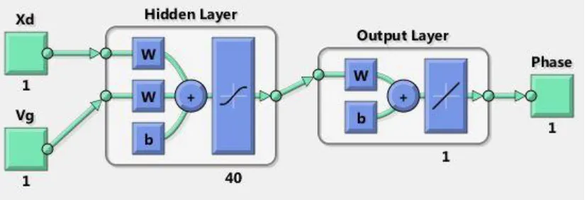
Figure 27 Inverse Plant Neural Network ... 46

Figure 28 Inverse plant training performance ... 47

Figure 29 Plant Identification at various velocities ... 48

Figure 30 Inverse plant neural network with velocity input ... 49

Figure 31 Velocity dependent inverse plant training performance ... 50

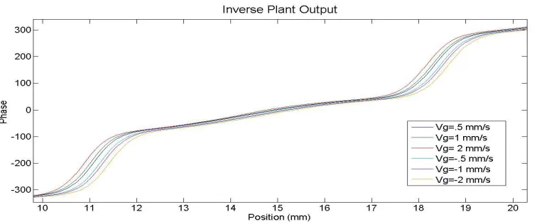
Figure 32 Inverse plant neural network output at different velocities ... 50

Figure 33 Neural network controller training network ... 51

Figure 34 NNc Training Data ... 52

Figure 35 Neural network controller training performance ... 53

Figure 36 Neural Network controller ... 54

Figure 37 Neural network controller with feedback validation ... 54

Figure 38 Neural network feedback controller output at different errors ... 55

Figure 39 System Flow Chart ... 57

Figure 40 Graphical interface control panel ... 59

Figure 42 INV controller results at various speeds ... 63

Figure 43 INV controller error at various speeds (6mm to 25mm) ... 64

Figure 44 iPID controller error at various speeds (6mm to 25mm) ... 65

Figure 45 iPIDv controller error at various speeds (25mm to 6mm) ... 67

Figure 46 IMC controller error at various speeds (25mm to 6mm) ... 68

Figure 47 IMCv controller error at various speeds (25mm to 6mm) ... 69

Figure 48 NNc controller error at various speeds (6mm to 25mm) ... 70

Figure 49 IMC response to a sine wave with plant offset ... 74

Figure 50 iPID response to a sine wave with plant offset ... 74

Figure 51 Modeled node positions as phase changes from 0 to 360 degrees ... 78

Chapter 1

Introduction

1.1 Motivation of Research

Non-contact manipulation is an important area of development because of its industrial applications in microassembly, its ability to manipulate corrosive or reactive materials, and its use in high temperature liquid processing. Using non-contact handling methods for containerless liquid processing eliminates contamination of the liquid due to a container therefore facilitating undercooling [1]. Microassembly of components becomes increasingly difficult using traditional grippers as the size of components shrink. In the assembly of MEMS, opto-elctronic microsystems and other microcomponents electrostatic, van der Waals, and surface tension forces become significant causing parts to adhere to traditional grippers not allowing proper part placement. There are several approaches to mitigating this problem of adhesion due to surface forces—one approach is non-contact manipulation.

handling in the food industry also has the advantage of avoiding end-effector contamination [2].

1.2

System Description and Project Focus

The focus of this project is to control the position and velocity of a small object in a standing wave acoustic levitation system. Travelling waves are produced by two

bolt-clamped Langevin transducers facing each other. The two transducers are driven at the same frequency causing a standing pressure wave to be formed between them as shown in Figure 1

Figure 1 Standing Wave between transducers

(1)

where r is the transducer radius[3].The nodes of the standing wave and the levitated pellet are moved by changing the phase relation between the two actuators. Several control schemes are compared and evaluated on their performance at various speeds and with the introduction of plant offsets. A particular emphasis is placed on the use of neural networks for plant identification and control. To see a graphical representation of all the node positions a finite element method is used to create a model of the system. The finite element model is

compared to the experimental results to determine modeling accuracy. The organization of the thesis will be as follow:

 Chapter 2 overviews current methods of non-contact handling and their limitations, describes the principles of acoustic levitation, neural networks, and the use of neural networks for control.

 Chapter 3 presents an ANSYS model, discusses data collection and preparation for neural network modeling, and shows how the control schemes are implemented in the experimental system.

 In chapter 4 the experimental setup is described, controllers are evaluated at different speeds and with plant offset, and the experimental results are compared to the

Chapter 2

Literature Review and Principles

2.1 Current Methods of Non-Contact Handling

There are several methods of non-contact handling each with its advantages and disadvantages. Magnetics, Electrostatics, Bernoulli’s effect, and acoustic forces are several of the physical principles exploited for levitating objects. An example application and a

description of the basic principle of each of these methods are outlined below. The focus of this thesis will be on standing wave acoustic levitation but a literature survey of several different methods of levitation is given by Vandaele, Lambert, and Delchambre in Non-contact handling in microassembly: Acoustical levitation[2].

Electromagnetic suspension systems utilize the forces between moving charges and magnetic fields characterized by Lorentz’s Law. Lorentz’s law gives the force on a charged particle as

(2)

Where F is the force exerted on the charged particle q by the electric field E and the cross product of the particle’s velocity and the magnetic field B. For a current carrying wire equation (2)can be simplified to

This formulation is used to calculate the amount of force generated on a wire coil by the suspended object or carrier plate. This force is controlled by changing the amount of current in the coil.

Chen, Tsai, and Fu [4] created a 2-d electromagnetic suspension actuator that used three permanent magnets and three coils to create a levitated platform. Their design is shown in Figure 2.

Figure 2 2-d Electromagnetic suspension actuator[4]

Although a reasonable analytical model can be created for this setup, calculations are too extensive for real time control. Instead the force is simply fitted to an experimental

specific regions. The adaptive aspect allows for control to be achieved even when the system is not perfectly known.

Electromagnetic suspension systems work well in applications where a high degree of precision manipulation is necessary. A levitated system is often easier to move precisely because of the low friction that allows for the stick-slip problem to be avoided.

Electromagnetic systems also have a high control bandwidth that allows for better system performance. A disadvantage of using a system based on magnetic forces is that the system is inherently unstable and requires active control. Another disadvantage is that a carrier

platform must be used unless the object itself is ferromagnetic or a very large magnetic field is generated[4]. Magnetic levitation also is not effective in high temperature applications because demagnetization of magnets at high temperatures.

Figure 3 Noncontact handling using Bernoulli’s principle [5]

A third method of non-contact manipulation is through electrostatic forces generated between two charges. The force generated between two particles is given by Coulomb’s law which is

(4)

Where is the permeability of freespace, q is the charge of the two particles and r is the position vector between the particles. Coulomb’s law is used to formulate the definition of an electric field as the force generated on a test charge per unit charge at a specific point or

(5)

Using the concept of electric field applied to a distribution of charges instead of a point charge by integrating Coulomb’s law over a volume allows the force between two charged objects to be calculated. Equations(4)and (5)show that the direction of the force is always toward the region of higher electric field. Electrostatic non-contact handling uses various methods of manipulating the electric field to control the forces applied to an object.

Figure 4 Electrostatic non-contact manipulation system[6]

The electrode is positively charged while the table is grounded causing a buildup of charge between the two just like a capacitor. This buildup of charge causes forces on the cylindrical objects in the direction of the greatest electrical field which is just under the electrode. The objects first line up with the electrode by moving from 1 to 2 and then move to be centered under the tip by of the electrode at 3 because it is closer to the table.

In the setup that was used there were several problems. The first is that the induced charges caused an increased adhesion force between the table and the object. Another

manipulation systems. Electrostatic methods can be applied to create a levitated system but because they use an attractive force they require active control to maintain stability[7].

2.2 Standing Wave Acoustic Levitation

Standing wave acoustic levitation (SWAL) systems often uses an acoustic transducer and a reflector to create a standing wave between the reflector and transducer. Another method of creating a standing wave is to use two transducers driven at the same frequency.

Figure 5 Acoustic transducer with reflector (top) Two acoustic transducers (bottom)

Figure 5 shows a diagram of a SWAL system that utilizes a reflector and one that utilizes two drivers. The lines between the transducers and reflector show the high and low pressure points of the standing wave. In this diagram the waves are shown as perfect plane waves but this is not the case for real systems. The area between each line is a pressure node where an object can be levitated. The numbers of nodes that form depend on the speed of sound and driving frequency. In Figure 5, a is along the axial direction and r is the radial direction.

Reflector

Ultrasonic transducer Piezo driver

Piezo driver

SWAL systems have several advantages over other methods of non-contact handling. The ability to levitate an object is independent of the whether the material is conductive, or magnetic therefore a large range of material can be levitated. The material limitation imposed by standing wave systems is that the object density must be below a critical value determined by the system parameters. Pressure nodes occur along the axial direction of a standing wave and it is these nodes that create a stable point to levitate objects. These nodes do not need to be controlled to remain stable unlike many magnetic and electrostatic systems. The third advantage of a SWAL system is that the object shape is not limited to flat or spherical objects, any shape object can be levitated as long as it is smaller than half the wavelength of the standing wave. A characteristic of a SWAL system is fluid flow around the levitated object which can cause heat and mass transfer. This heat and mass transfer can be beneficial in experiments where part cooling is desired but may not be desired in high temperature experiments. Fluid flow around the part also means that while the part is stable it does rotate.

The force that levitates an object is due in part to the acoustic radiation forces on the object. Early work on acoustic radiation pressure was done by King who developed the equations describing the pressure on small, incompressible spherical objects. Small defined by King is the radius of the object being much smaller than the wavelength of the standing wave. The wavelength of the standing wave is given by

(6)

where Cs is the speed of sound in the medium and is the driving frequency.

expression developed by King for the average pressure on a small sphere from traveling waves is

| | ( )

(

)

(

)

(7)

The pressure from traveling waves is a function of the density of the surrounding median, , the density of the object, , the wavelength , and A is assumed to be the wave amplitude. The pressure on a rigid sphere from a standing wave is given by the function

| | ( ) ( )

(

)

(

)

(8)

The pressure from a standing wave has a similar form as the traveling wave but there are several important differences to note. The first difference is that the standing wave pressure as expected is dependent on the position in the wave. This is given by the term,

where h is the distance from a pressure node. The reason standing waves generate more force than traveling waves is because of the term. The circumference of the object must be much less than the wave length in order for levitation to occur or mathematically

extended King’s work to compressible spheres[9]. For objects with King’s model

looses accuracy and must be modified as suggested in [10] with this modification the model is accurate as long as .

The analysis done by King and others describes the forces along the axial direction between the actuators but there is another force that acts in the radial direction. The force in the radial direction is towards the actuator centerline at the pressure nodes. There are several phenomena that lead to the development of this force. In the idealized case of plane waves there would be no distribution along the radial direction but realistically perfect plane waves are not created causing a non-uniform pressure distribution. Another source of this radial force is from acoustic streaming caused by the non-uniform pressure distribution along the radial direction of a node [11]. Tuziuti et al. relate this idea of a non-uniform pressure distribution along the radial direction to there being a non-uniform velocity distribution. Using this velocity distribution and an equation that relates radiation force to potential and kinetic energy the force is quantified in the radial direction [12]. The radiation force equation used was first developed by Nyborg and is

〈 〉 〈 〉 (10)

where〈 〉 and 〈 〉 are the time averaged kinetic and potential energy of sound respectively. The B in equation (10) 1010is defined by the density of the medium and object and is

(11)

direction is a Gaussian distribution, g(y). If the distribution of velocity is Gaussian then the 〈 〉 and 〈 〉 terms become

〈 〉 ( ) (12)

〈 〉 (13)

(14)

Equations 10-(14)are combined to form the equation for the radiation force in the radial direction which is

( ) ( ) ( ) (15)

A in equation(15) is the sound pressure amplitude and is the standard deviation of the

Gaussian velocity distribution[12]. A plot of this force over a range of is shown in Figure 6.

The force in the radial direction causes an object to be pushed toward the centerline of the cylindrical actuators. There are two equilibrium points for the object to levitate at but the centerline is the most stable point. This radial centering force combined with the stable axial position makes standing wave acoustic levitation an attractive levitation technique.

2.3 Neural Networks

Neural networks (NN) or Artificial neural networks (ANN) as they are often called are a tool that is based on the biology of the nervous system. A biological neuron is

composed of four main parts: dendrite, synapse, soma, and axon. A diagram of a biological neuron is shown in Figure 7.

Figure 7 Biological Neuron

axon is the device by which the neuron passes its signal to other neurons. The connection of many of these neurons creates a powerful network that is capable of processing complex information and acting on it[14].

Artificial Neurons have a similar topology as their biological namesake. A model of an artificial neuron is shown in Figure 8.

Figure 8 Artificial Neuron

The artificial network collects signals and multiplies each signal by a distinct value called a weight therefore assigning certain inputs more weight than others. The signals are then summed and processed just as in the soma of the biological neuron. The output of the neuron shown in Figure 8 does not branch but the output of one neuron could also be the input to multiple other neurons. A single neuron is limited in its ability to process signals and it is only through the connection of several neurons forming a network that a powerful tool is developed [15].

Neural networks can be applied to a broad range of applications including robotics,

W

W

W

problems that NNs are good at solving. Control of robotic systems is difficult using conventional controllers because of the nonlinearity and changing system parameters. The inverse kinematics of a robotics system is a particular difficulty in robotic controls. The inverse kinematics problem in robotics is given a desired end-effector position find the joint variable that lead to this end-effector position. The difficulty is that there may be multiple solutions, a single solution or no solution at all to reach the desired end-effector position. Traditionally there have been several methods of solving the inverse kinematics problem including algebraically, geometrically, and using an iterative method. Each of these methods has drawbacks and limitations, and a better method of solving for the joint variables is desired. One solution is to formulate the inverse kinematics problem as an optimization problem which is well suited to being solved in real time by a neural network [16]. This example illustrates one way in which NNs can be applied to controls problems.

Forecasting means linking the interdependence of variables in order to predict other variables. Financial markets are influenced by tangible assets such as buildings and land but they are also influenced by the harder to model in-tangible assets such as patents, copyrights, and brand recognition. Finding how these variables are linked allows for one to build a model and predict future outcomes. One method that is being used to find the relationships among these many variables utilizes the powerful function approximation capabilities of NNs to develop models and make predictions. NN models have the advantage of not being fixed around a certain formula, which gives them the ability to adapt to changes in the market [18].

The first mathematical model of a neuron was developed by Warren McCullouch and Walter Pitts in their 1943 paper. The McCulloch-Pitts model is governed by a set of five rules:

1. The activity of a neuron is an all or nothing process

2. The activity required for a neuron to fire is independent of previous activity 3. The only delay within the system in the transfer of the signal

4. A neuron’s firing threshold will increase if an inhibitor signal is active 5. The structure of the network does not change with time

The mathematical realization of these rules is

∑ (16)

where w is a fixed vector of weights, x is the set of input signals, and l is the required activation energy. The output of the neuron is given by

Figure 9 Step Function

The function shown in Figure 9is often called the activation function of the neuron. This activation function is what decides if the input signals are going to be passed on or in other words if the neuron is going to fire. There are many possible activation functions, and some of the more common functions include the sigmoid function given by

(18)

and shown in Figure 10. The sigmoid function is popular because it is differentiable which is useful when trying to determine the weights.

Another type of activation function a piecewise linear function such as

{

(19)

From the McClloch-Pitts model came the Perceptron model developed by Frank Rosenblatt in 1958. The Perceptron has a similar structure as the neuron shown in Figure 8 and similar equation as the McCllouch-Pitts model. The biggest difference is that in the Perceptron the weights are tuned parameters. The Perceptron is tuned by using a sample set of data that includes inputs and desired outputs. The difference between the desired output and the actual output is used to change the value of the weights. The weight update rule used in Rosenblatt’s Perceptron is

(20)

Where is the current weight of the ith input, is the learning rate and d is the desired output [20].

Figure 11 Single layer feedforward neural network

For the single layer network Sn is the nth input and Wi,n is the weight of the nth input going

to the ith neuron. The number of outputs O is the same as the number of neurons in the network. This type of diagram becomes cumbersome when describing more complex networks therefore an abbreviated diagram that utilizes vectors and matrices is commonly used.

Figure 12 Abbreviated single layer diagram

S

[nx1]

W

[ixn]

f(WS+b)

[nx1]

[ix1]

O[ix1]

S

S

S

W

W

f(Σ signal)

f(Σ signal)

f(Σ signal)

O

O

For the abbreviated diagram the input becomes a column vector that is multiplied by a weight matrix. The b column vector is called the bias term which is a vector of constants that shifts the activation function for each neuron.

Adding additional layers is one way of increasing network capabilities. When three or more layers are used and there is no feedback from previous layers the network is called a multi-Layer feedforward network or multi-layer perceptrons (MLPs). These multilayer perceptrons have become the most widely used architecture particularly in the systems and controls field[21].Figure 13shows a MLP with a single hidden layer.

Figure 13 Multilayer Perceptron

The multilayer perceptron is usually broken into three parts. The first part is the input layer which consists of a weight matrix, IW, and an activation function. The last part of the network is called the output layer and it consists of the weight matrix, Wo, and the output

training time and a MLP with a single hidden layer can approximate any function arbitrarily well with enough perceptrons [22].

A single perceptron can effectively be trained by minimizing the error between the input and output using equation(18). Training multi-layer networks with several neurons and multiple layers becomes a much more difficult task than the training of a single perceptron. To accomplish this task a back-propagation algorithm can be utilized. The back-propagation algorithm looks at the last layer of the network first and for each output finds the error between the output and desired output and calculates how changing the weights of the input impacts the output. The algorithm then changes the weights in the opposite direction as the calculated gradient, thus causing the overall system error to decrease. For the hidden layers a similar process is used that says the error of a neuron is the sum of the error of the neurons connected to its outputs times their weights. This hidden layer error calculation is used to come up with an error gradient and the weights are changed in the opposite of the maximum gradient. By continuing this process over the entire set of training data the MLP network begins to model the unknown input output function.

A variant of back-propagation that speeds up convergence is the Marqurdt-Levenberg algorithm. This algorithm combines back-propagation with a quasi-Newton approach.

minima and then slowly converge to the precise minimum. A thorough examination of the back-propagation method and the quasi-Newton method can be found in Training

Feedforward Networks with the Marquardt Algorithm written by Hagan and Menhaj[23].

2.4 Neural Networks for Control

Neural networks can be applied to the field of controls in a variety of ways. Networks can be used for modeling unknown nonlinear systems, feedback controllers, inverse plants, predictive controllers or as adaptive controllers. This thesis will focus on the use of neural networks for plant identification, using the inverse plant in conjunction with a PID control scheme, an internal model control scheme, and a neural network feedback controller. All of these controllers can be trained offline and do not utilize online adaptive techniques.

The simplest type of controller that can be implemented using a neural network approach is an inverse plant controller. A diagram of a system using an inverse plant as a controller is shown in Figure 14.

This controller relies on being able to model the inverse dynamics of the plant using input output pairs collected offline. The input vector Xd is the set-point of the plant and for many

systems will contain previous set-points of the system. While this is a simple controller to implement one flaw is that there is no feedback and changes in the plant over time and disturbances will reduce the effectiveness of the controller. To increase disturbance rejection and tracking abilities the controller needs to be formulated in such a way that feedback can be introduced. An inverse plant controller with feedback is shown in Figure 15

Figure 15 Inverse Plant with Feedback

The control input to the plant at time n can be formulated as

(21)

where the function is trained from input output data of the plant and the filtered error is given by

where the filter F(.) applied to the error is a first order filter of the discrete form

(23) is the tuning parameter that changes the amount of filtering applied where is not filtering and is a no-pass filter. The Z-1

blocks are discrete unit time delays. This control scheme allows for compensation to be made for the differences between the plant and inverse plant or disturbances.

In the previous control scheme the error is only dependent on the set point and output of the plant but another formulation would make the error dependent on previous error values, the plant output and the set-point.

Figure 16 Internal Model Controller

Figure 16 shows an internal model controller (IMC) that compares the output of the plant to a set-point modified by the previous error. The plant input is governed by equation (21) where the error is given by

where ̃ (n) is the modified set point that accounts for modeling error and disturbances and is given by

̃ ₍₂₅₎

Three properties that make IMC a good choice of a control scheme are

1. If the controller and plant are stable and the internal model perfectly represents the plant, then the closed loop system will be stable.

2. If an inverse plant model exists and is used as the controller, and the system is closed loop stable, then with no disturbances perfect control is achieved.

3. If the controller gains are inverse of the internal model gains then offset-free control is achieved for constant set points [24].

While a perfect model can never be achieved accurate models can be developed using neural networks to model the inverse properties of a system. One advantage of the IMC controller over the feedback controller shown in Figure 15 is zero steady state offset is achieved.

Figure 17 Inverse plant with PID control

The input into the inverse plant is given by

̃ ∑ (26)

where the error is given by

(27)

An advantage of this controller over a simple feedback system is that because it incorporates integral control steady-state offset can be eliminated. Also, this controller has the capability to respond faster to error than a simple feedback controller. A disadvantage of trying to use a linear control technique on a nonlinear system is that finding gains that work over the entire system space is impossible for many systems.

feedback is this includes a neural network that uses the set-point and error to find the input into the inverse plan. The nonlinear properties of neural networks allow the control action to depend on the region and not just the error.

Figure 18 Feedback Neural Network controller

This multi input controller is trained from the input and outputs of the inverse plant

controller. Figure 18 shows the NNcont and NNplant-1 as separate blocks but in reality it is possible to combine them into a single larger neural network.

To manipulate any levitated object some form of control is necessary. With magnetic and electrostatic levitation active control is necessary just to create a stable levitation

of modeling the levitation system from experimental data. The models created can be applied to form a control system capable of handling the acoustic nonlinearity. Neural networks are a possible way to model the system from experimental data but a model based on acoustic principles is also useful in understanding this system. To model and control this complicated system both a neural network and finite element model are created. The

Chapter 3

Finite Element and Neural Network Modeling

3.1 ANSYS Model

Analytically modeling an acoustic system for a non-idealized case is not a trivial task. Since the pistons used in this experiment are not baffled they do not create perfect plane waves as in the idealized case. Also it is desired to know the pressure distribution along the radial direction not just at the centerline. A finite element model is created to view the pressure distribution and node locations between the actuators at different phases. The first step to creating a finite element model is to define the geometry of the system. After the geometry is defined the material properties, element types, system loadings, and analysis mode are selected. The final step is to create a mesh for the system and solve for the desired outputs.

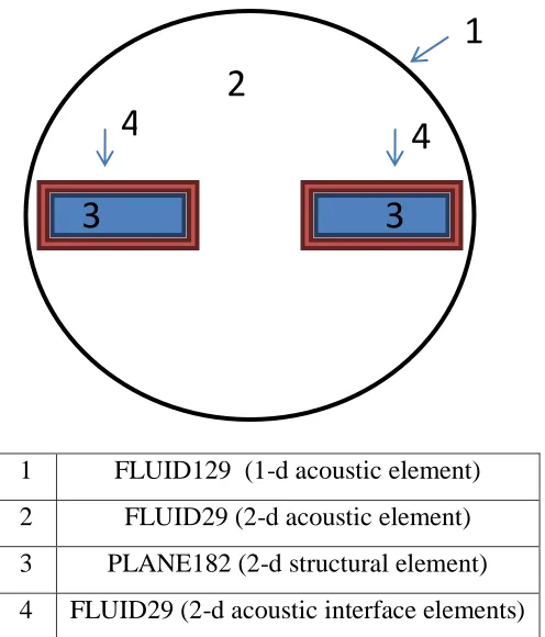
The model for the acoustic system will be a 2-d model of the cross-section of the cylinders. The geometry for this system will simply consist of a circular air region, and two aluminum cylinders. Each region is defined by a certain element type and physical

1 FLUID129 (1-d acoustic element) 2 FLUID29 (2-d acoustic element) 3 PLANE182 (2-d structural element) 4 FLUID29 (2-d acoustic interface elements)

Figure 19 ANSYS model and element types

The gap between the cylinders is 3 cm and the diameter of them is 2cm. The circular region is the air region which has a radius of 9cm. The first element that is used is the 1-d acoustic element that surrounds the air region—this element is an absorbing boundary condition. An absorbing boundary condition is used to simulate a large open space that does not reflect sound waves back toward the actuators [25]. The second element that is used defines the air region and is the 2-d acoustic element called FLUID29. The 2-d acoustic element is based on the wave equation

(28)

1

2

3

3

where C is the speed of sound in the fluid, P is the acoustic pressure and is a function of position and time. A discrete form of this equation can be written as

[ ]{ ̈ } { } (29)

The matrix is the fluid mass matrix and is calculated using the pressure shape function {N} and the equation

∫ { }{ } (30)

The element stiffness matrix is calculated by the equation

∫ (31)

Where the matrix [B] is the dot product of the gradient and shape function and is given by

{ } (32)

Equation (29) describes the 2-d acoustic elements that are only in contact with other acoustic elements but region 4 is in contact with structural elements as well. A modification is made to the standard acoustic element that couples it to the actuators allowing for fluid structure interaction. The coupling term at the fluid structure interface is that the pressure gradient of the fluid is equal to the density of the fluid dotted with the acceleration of the structure or

{ } { } { } (33)

where {n} and {u} are the normal vectors of the fluid and structural surface respectively. In discrete form this coupling term becomes

{ ̈} ∫ { }{ } { } { ̈} (34) This term is added to the left side of the discrete wave equation to create the acoustic

[ ]{ ̈ } { } { ̈} (35) Region 3 uses a simple 2-d structural element defined by Young’s Modulus and Poisson’s ratio to model the acoustic actuators. The structural element also has a coupling term that links its governing equation to the pressure gradients at the fluid structure interaction. The goal of this thesis is the investigation of the standing acoustic wave not the structural vibration therefore a detailed analysis of the structural equation is omitted. For a more detailed explanation of the acoustic and structural elements see the theory reference section of the ANSYS help documentation.

To completely define the model not only must the element types be created but the material properties and loadings must be set as well. Table 1 gives the properties that are used to define the model shown in Figure 19.

Table 1 Physical properties

Aluminum Air Loadings

E=60e9 Pa Speed of sound=340 m/s Frequency=26.7 kHz Poisson’s ratio =.35 Density=1.2 kg/m^3 Amplitude= 7um

Mu=0

Figure 20 Meshed acoustic system model

Once the model is meshed a harmonic loading is placed on the inside faces of the actuators while the outside faces are fixed in space. The load is defined such that the inside faces move toward each other at the same speed when the phase and time are 0. The phase between the actuators is changed by modifying the load on the right actuator face. The harmonic load is written as a complex number where the real and imaginary terms define both the magnitude and phase of the load. For this analysis the magnitude is kept constant but the phase is

increased from 0 to 330 degrees on the right face. The positions of the left and right actuators are given by the equations

₍₃₆₎

where UL is the left actuator, UR is the right actuator and is the phase between them.

Figure 21 Pressure distribution at 0 degrees phase

Figure 22 Pressure magnitude along centerline at several phases

In this plot the bold points each represent a node and depending on the phase there are either 3 or 4 nodes between the actuators. The number of nodes between the actuator is determined by the frequency and gap distance. As the phase is increased the position of the nodes moves to the right and Figure 22 shows that when a phase shift of 270 degrees is reached the node position is closer to the next 0 degrees node then the original node. What this means is that when the phase is shifted 360 degrees with a levitated object the object moves to the next node therefore the object can be moved from one side to the other by increasing the phase and moving node to node.

In the results section the ANSYS model will be compared to the experimental results. The ANSYS model gives values for the pressure magnitude between the actuators but it does not include the near field acoustic effect, which is a significant factor for the gap size being used. In the experimental system it is difficult to take pressure measurements in the

model will not be compared. What will be compared are both the distance between the nodes in the model and the experiment and how the node position changes with phase.

3.2 Neural Network Modeling

Neural networks can be trained either ‘online’, ‘offline’ or a combination of both. Online training consists of an untrained network being implemented into a control system and weights and biases being updated based on actually using the plant. Offline training is using data either collected from the actual system or from another model to train a neural network before it is implemented. Often networks will be initially trained offline and then

implemented with the ability to continue training or ‘adapt’ to the actual plant. This project will focus on using offline methods to create neural networks. The MATLAB Neural Network toolbox is used to construct and train the networks created in this project.

After the data is collected training speed and accuracy are optimized by preprocessing the data. The first preprocessing function is to delete inputs that are constant for the whole set of data because they do not contain any information about how the plant responds. The second preprocessing function is to map all the data between -1 and +1. The reason for this is that the sigmoid function shown in Figure 10 is often used in the hidden layer of a network and it quickly saturates when the inputs are large unless the input gains are very small. This saturation causes a small gradient in the weight updating process thereby increasing the required training time. The algorithm used by MATLAB to accomplish this mapping is given by

(37)

where x is the data value to be mapped and xmin and xmax are extremes of the data and y is

the data sets may not have been divided well. Typical data division percentages are 70% for training, 15% for validation and 15% for testing [26].

The data collected to determine the relationship between transducer phase and node position of the SWAL system is collected over the entire feasible control range. If the transducers are 30mm apart then the region of control is from 5mm to 25mm from the left face of the actuator. The procedure for initializing the system to be able to collect consistent data is given below:

1. Allow the system to warm up by tuning the transducer on and waiting a few minutes 2. Set the channels 1 and 2 phase to 0 degrees.

3. Align the phase between the two channels of the signal generator by pressing the ‘align phase’ button on the signal generator.

4. Levitate the Styrofoam ball between the actuators at the first node to the right of the center point (about 18mm).

5. Increase the phase of channel 1 on the signal generator until the ball is centered. If the system is warmed up then this will correspond to about 160 degrees.

constant. A plot of the position versus phase data collected in this manner and used to create a NN and inverse plant is shown in Figure 23.

Figure 23 Plant Identification from Phase

Figure 23clearly shows that the system is nonlinear and that there are regions where

Figure 24 Standard deviation of position over the control region

The standard deviation of position shows the amount the object oscillates due to the changing forces on it. Figure 24 shows that there are certain regions where the object will oscillate more and that these regions are the same in which the object position is sensitive to phase change. The standard deviation plot is created by collecting several position points at 10o phase increments and finding the average and standard deviation of those points. The oscillations occur much faster than the data sampling rate and therefore they cannot be controlled. This means that the optimum controller for this system will have error that approaches the standard deviation of the system.

coefficient, α, different values are tested with the same controller to see the impact of filtering. The end goal is to minimize error therefore the filtering coefficient that minimizes error over the operating range is selected.

Figure 25 Effects of filtering on the controller error

use for this experiment because it performs well at different velocities and is a good balancing point between high frequency attenuation and lag.

3.3 Control Implementation

Control of both the position and velocity of the levitated object is the goal of this control system. The first goal is to be able to command a set position and have the object levitate at that position with no steady state error. The second goal is to be able to specify the velocity with which the object moves to the desired location. To achieve this second goal a path must be generated that specifies a desired position at a desired time. A point is

generated one step ahead for a constant velocity using the equation

(38) Where Xo is the initial object position and is the time it take for one cycle of the control

loop. It is also desired for the object to be able to follow a sinusoidal path based on a center point, frequency and amplitude. The equation that generates the desired path is given by

(39) Where Xc is the center position about which the object will oscillate. A comparison between

this desired position and real position is how the error is calculated and the controllers evaluated.

Figure 26 PID control diagram

The PID block is governed by

∑ (40)

Where ts is the time between samples. Uc is the control action of the PID block from the error

term. Uo is the expected control input for the desired position and is calculated assuming the

plant is linear by using the slope between the two endpoint of Figure 23. For this system Uo

is

(41)

The most effective gains found for this system are Kp=35, Ki=.5, and Kd=0. No derivative

gain is used because it only amplifies the oscillations that the filter tries to attenuate. The second type of controller that is implemented is an open-loop inverse plant controller shown in Figure 14. To create this inverse plant the data shown in Figure 23 is used to create input output pairs where the input is position and output is phase.

Plant

Filter

-+

+

+

Xd

U

X

e

PID

u

Figure 27 Inverse Plant Neural Network

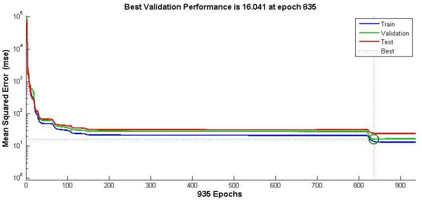
Figure 28 Inverse plant training performance

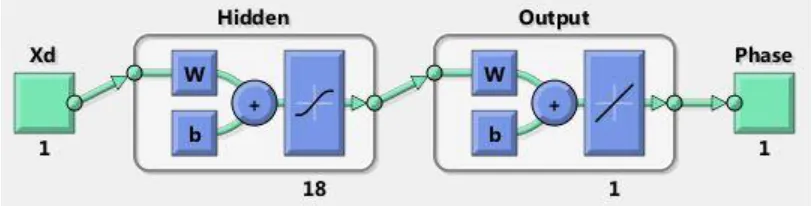
The hidden layer consists of 18 neurons with a sigmoid activation function while the output layer consists of a linear activation function. There is only a single output therefore the output layer has a single neuron. This inverse plant is all that is needed to create the

controllers proposed in Section 2.4 except for the feedback neural network controller shown in Figure 18.

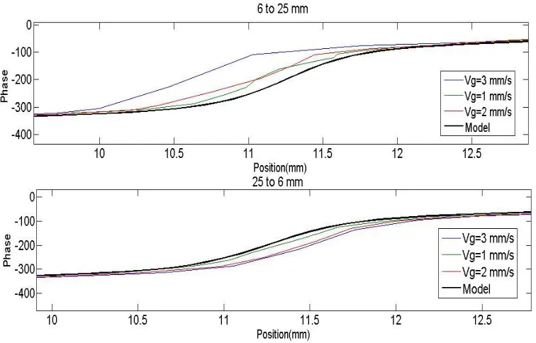
The top plot shows the object traveling from the 6mm position to the 25mm position—left to right, and the second plot shows the object traveling from right to left.

Figure 29 Plant Identification at various velocities

In traveling left to right the top plot shows that the model always under-predicts the

Figure 30 Inverse plant neural network with velocity input

This neural network has the same structure as the network in Figure 27 except that this has multiple inputs and more neurons in the hidden layer. The velocity dependent network is trained using the phase and position data collected when moving the object at various speeds. For this network 1517 data points are collected and again are separated randomly into

Figure 31 Velocity dependent inverse plant training performance

One possible reason that this shift occurs is that the object itself affects the acoustic field and if the object is commanded to change quickly it is expected that it will disturb the

surrounding acoustic field more. This added disturbance can impact the acoustic near-field causing the plant behavior to change.

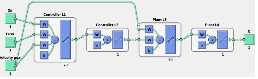
Another controller that is tested is the neural network controller with feedback which is shown in Figure 18. This controller has desired position, goal velocity, and error feedback as inputs. Training this network offline is not as straightforward as training the inverse plant. Training this network requires having a plant model and cascading this with the controller. A diagram of this cascaded training network is shown in Figure 33.

Figure 33 Neural network controller training network

layers are fixed during training because it is the controller which is to be trained not the plant. The output of the training network is position, X, which is trained to be the same as the Xd value. The only way the Xd input and X output can match is if the controller weights change so that it becomes both an inverse plant and feedback controller. The weights attached to the Xd and velocity goal inputs will be the model of the inverse plants just like in Figure 30. The error input weights are what will become the feedback portion in the controller. The training data used is from the open-loop inverse plant controller and is shown in Figure 34.

Figure 34 NNc Training Data

The actual process of training the feedback neural network controller takes more time because there are four layers through which the error must back-propagate. The Marqurdt-Levenberg algorithm is used to optimize the performance of this network. The network is trained for 165 epochs and the best epoch was 65 and has a root mean square error of .077mm. The performance measure of this network is in mm instead of degrees like the other networks because the training network contains both a controller and a plant model which has an output of position. The performance progress of the training, validation and testing data sets are shown in Figure 35.

Figure 35 Neural network controller training performance

Figure 36 Neural Network controller

After training the network with the data shown in Figure 34 the controller is tested by comparing the error of the training data, Xd-X, to the error produced by the simulated plant

when the trained controller is applied. The inputs to the controller are the first 500 training data point and the results of the simulation are shown in Figure 37

The simulated results show the controller reduces the amount of error in the training data which indicates that it is correctly modeling the inverse plant and compensating for error. To see the effects of the error feedback on the controller, output plots of the network over the control region at a constant velocity and different errors are used.

Figure 38 Neural network feedback controller output at different errors

constant error. In the areas where the system is sensitive to phase changes, such as from 12mm to 17mm, the amount of control action is small. From 18mm to 20mm the system is not as sensitive to phase change therefore a greater amount of phase change is required for a constant error. Figure 38 shows that between 10mm and 12mm positive error is at a lower phase angle then the error free output—this is the opposite of what is generally wanted. The network outputs in this region could mean several things the first is that the plant behaves differently over this region, second that there were not enough training data points in this region to create a good general model, or third that more training of the network is necessary.

The finite element model and the neural network model both show that it is possible to move a levitated object between the actuators gap by manipulating the phase between the actuators. To create an accurate neural network model data needed to be carefully collected and used to train the networks. The data collected showed that the oscillations in the acoustic system require a filter to be applied to the position sensor in order for effective control to be possible. When testing the controllers it was noticed that as the object speed increased the plant behaved differently therefore a set of models were created to incorporate these

dynamics. After the controllers are created and implemented in the experimental setup their performance needs to be evaluated and compared. Chapter 4 discusses how the controllers will be evaluated at different speeds and plant offsets. Chapter 4 also compares the

Chapter 4

Results and Conclusion

4.1 Experimental Setup

In this experiment various control schemes are used to manipulate a levitated object between two bolt clamped Langevin type transducers. To implement control schemes with feedback and to run the transducers five components are needed.

Figure 39 System Flow Chart

The first part of the system shown is a computer that runs a MATLAB GUI that calculates the control action and communicates that information to the signal generator. The GUI was created by Joong-Kyoo Park [3] and control functionalities were added for these experiments. The signal generator is a Tektronix AFG 3022B signal generator which is able to produce two sine waves of different phases. The signals are then amplified 100 times by two Trek Piezo drivers. The amplified signal is then passed to the two transducers which produce the standing wave. The transducers are set up so that 0 degrees phase difference on the signal generator means that they are moving at the same speed but in opposite directions. A camera takes a picture of the gap between the actuators which is sent to the computer. The ball is white and the transducers are black with red control points that allow the computer to calculate the position of the ball with respect to the lower corner of the left actuator. With the updated position information the computer calculates the next control input.

The experimental setup is the same used by Park and Ro in Non-contact

Manipulation of Light Object Based on Parameter Modulations of Acoustic Pressure Nodes

[3].For this particular system Park and Ro found several specific parameters that optimize acoustic power. The driving frequency used is 26.7 KHz because that is the natural frequency for the transducers. Using the natural frequency leads to the greatest amplitude of

displacement which is 7μm. To achieve levitation over a gap of 3cm the voltage of the signal generator is set to 4 volts peak-to-peak.

To interface with the system a GUI is created in MATLAB. Using this GUI

tracking, changing control parameters, and saving data. An image of the GUI is shown in Figure 40.

Figure 40 Graphical interface control panel

The top left corner of the GUI shows the image of a levitated ball being tracked. The

actuator block. The controls block allows for different control algorithms to be tested, different PID gains, and filtering changes. The control block also allows changes in the goal velocity and set-point for each run. Data from each run is saved and stored in a MATLAB data file. The system collects phase, x and y position, time, error, desired position, and for the PID controller control action due the PID gains.

4.2 Controller Response at Various Speeds

In this project there are eight different control setups that are tested with various gains and filtering values. To clearly distinguish which control setup is being used a naming

convention is given in Table 2.

Table 2 Control Scheme Names

Abbreviated Name Inverse Plant Used Block Diagram

PID n/a Figure 26

INV Velocity Independent Figure 14 iPID Velocity Independent Figure 17 IMC Velocity Independent Figure 16 INVv Velocity Dependent Figure 14 iPIDv Velocity Dependent Figure 17 IMCv Velocity Dependent Figure 16

Several of the controllers require the use of an inverse plant and there are two different types of inverse plants that are used. The first inverse plant is only dependent on position and is shown in Figure 23. The second inverse plant is dependent on the goal velocity and is shown in Figure 32. The only thing using this velocity dependent plant changes is each control scheme has multiple inputs—the first being position and the second being desired velocity.

Each controller is tested by moving the levitated ball from the 6mm to the 25mm position at various velocities. The velocities most often used are .5 mm/s, 1 mm/s, and 2 mm/s but some testing was done at 4 mm/s as well. The plant responds differently when moving left to right then when moving right to left therefore tests are done in both directions. To compare the results of one controller to another steady state error once the object has reached its set-point is looked at as well as the root mean square of the error. The RMS error value is calculated using

√∑ ( )

(42)

where n is the number of data points collected during one run.

Figure 41 PID controller results at various speeds

There are six lines in Figure 41 which show how the PID controller performs at .5 mm/s, 1 mm/s, and 2 mm/s. The plot shows a straight line which is the desired trajectory and the actual trajectory. The results in Figure 41 show that while the object is able to accurately follow the desired path there is significant periodic error. This periodic error is expected because the system is nonlinear and therefore a gain that works well in one region would not work well in another. This controller does have integral control therefore it settles to the set-point value.

Figure 42 INV controller results at various speeds

Adding the inverse plant even though this is an open-loop controller resulted in a much better performance than the PID controller. That is because the inverse plant takes into

Figure 43 INV controller error at various speeds (6mm to 25mm)

The position vs. error plot shows that most of the error is positive meaning the controller tends to underestimate the amount of phase needed for a certain position. The second thing to notice is the trend of underestimating the control needed increases as the velocity goal

increases. To quantify this trend the error of each run was summed and divided by the number of data points in that run. The result of this is an error average of .044mm, .12mm, and 18mm for velocities of .5 mm/s, 1 mm/s, and 2mm/s respectively. This plot is only for going from 6mm to 25mm—a plot of going 25mm to 6mm would show error that was mostly negative. The reason the slower speed run shows a noisy error signal is because data points were taken at closer intervals then in the faster traveling runs. If the sampling frequency were greater the higher speed runs would also be noisy. The RMSe of a run using the INVv

The inverse plant models can be combined with a PID controller to form the iPID and iPIDv controller. The effectiveness of the iPID controller is shown in Figure 44.

Figure 44 iPID controller error at various speeds (6mm to 25mm)

The iPID error plot shows that adding feedback drives the error to be centered about 0. Multiple gains were tried but it was found that the best results were from Kp=1, Ki=0, and

Table 3 RMSe of several different PID gains

No. Xo (mm) Vg (mm/s) Kp KI KD RMSe (mm)

1 6 0.5 1 0 0 0.078

2 6 0.5 1 0.1 0 0.118

3 25 0.5 1 0.1 0 0.131

4 6 1 1 0 0 0.089

5 6 1 1.1 0.1 0 0.187

6 25 1 1 0.1 0 0.195

7 6 2 1 0 0 0.145

8 6 2 1.05 0.05 0 0.164

9 6 2 1 0.05 0 0.167

10 25 2 1 0.05 0 0.170

11 25 2 1.05 0.1 0 0.224

12 6 2 1 0.1 0 0.285

13 25 2 1 0.1 0 0.302

14 25 2 1 0.2 0.02 0.321

15 6 2 1 0.2 0.02 0.329

16 6 2 1.2 0.2 0.02 0.339

17 25 2 1.2 0.2 0.02 0.358

Table 3 shows that the best performance based on RMSe of the gains tried was when Kp=1.

from 6mm to 25mm while the range of phase is -400 degrees to 400 degrees—this means that the gains for feedback directly into the plant need to be large to have the same impact.

The next step is to compare the iPID controller performance to the iPIDv controller that uses the velocity dependent plant. Again the best results were obtained when Kp=1 and ,

Ki=0, and Kd=0. Figure 45shows a large amount of error around the 25mm position this

25mm position corresponds to the first few seconds of each run because this run goes from 25mm to 6mm.

Figure 45 iPIDv controller error at various speeds (25mm to 6mm)

Figure 46 IMC controller error at various speeds (25mm to 6mm)

One thing to notice about the error of the IMC controller compared to the PID controllers is that as the speed in increased the amplitude of the error does not increase significantly. Figure 44 of the iPID controller clearly shows more error peaks as the velocity increases and the error curve magnitude increases as velocity increases.

Figure 47 IMCv controller error at various speeds (25mm to 6mm)

Comparing the results of the different controllers by sight is difficult even using a plot of the errors. Table 4is used to numerically compare the performance of each controller based on the RMSe and the peak error amplitude.

Figure 48 NNc controller error at various speeds (6mm to 25mm)

The error versus position plots are useful when looking at characteristics of a single controller but to look at multiple controllers it is useful to define a performance function and compare the controls based on that. For this experiment the RMSe is the performance function used to evaluate the controllers. Although this is a useful performance measure it does not show if there is a steady state error once the object reaches the set-point. Table 4 contains the RMSe for each of the plots shown in this section. The column labeled emax is the

Table 4 Controller performance measure

No Controller Xo (mm) Vg (mm/s) RMSe em (mm)

1 iPIDv 25 0.5 0.0742 0.3

2 IMCv 25 0.5 0.0781 0.22

3 iPID 6 0.5 0.0781 0.15

4 IMC 25 0.5 0.0860 0.23

5 INV 6 0.5 0.1304 0.45

6 INVv 25 0.5 0.1732 0.45

7 NNc 6 0.5 0.1949 0.38

8 PID 25 0.5 0.5477 1.2

9 IMCv 25 1 0.0707 0.2

10 iPID 6 1 0.0894 0.21

11 iPIDv 25 1 0.0949 0.2

12 IMC 25 1 0.0985 0.25

13 INV 6 1 0.1581 0.45

14 INVv 6 1 0.1788 0.37

15 NNc 6 1 0.1949 0.4

16 PID 25 1 0.5291 1

17 IMCv 25 2 0.1342 0.3

18 IMC 25 2 0.1378 0.31

19 iPID 6 2 0.1449 0.45

20 INVv 25 2 0.1732 0.48

21 iPIDv 25 2 0.2049 0.33

22 NNc 6 2 0.2098 0.43

23 INV 6 2 0.2324 0.5

The table is sorted by the goal velocity and the RMSe value therefore each velocity is

grouped together with the first in the group having the least amount of error. The highlighted rows show the best performance at each speed is a controller that includes the velocity dependent plant. The performance improvement is not large and does not guarantee a minimum value of emax.

4.3 Controller Response to Plant Offset

When assessing a controllers it is not only important to see how well it performs under ideal conditions but also how it responds when the plant is different than modeled. In an actual system the plant will always be different from the model because perfect plant identification is impossible. Even if an excellent model is developed time, cyclical loading and heat take their toll on any apparatus causing plant and model mismatch. To simulate this wear the controllers are run with a plant offset. The phase is what is being controlled

therefore it is the phase that will be changed. In section 3.2 Neural Network Modeling the procedure for initializing the system is described. In step five the phase of channel one of the signal generator is increased until the object is centered between the actuators. After step five is done the phase is then increased to the desired offset amount.

Figure 49 IMC response to a sine wave with plant offset

The IMC is able to follow the sinusoidal path at any offset but at 30o or greater the object becomes less stable and oscillates at certain regions. The other thing to notice is that the controller is able to quickly settle at the 30sec set-point without any offset.

The iPID controller performs better than the IMC when the plant offset is zero as seen by the close match between the blue and green line. As soon as there is a plant offset the iPID controller is unable to compensate and undershoots the desired position in some regions and overshoots the desired position in others. After the run is complete at 30 seconds the desired set-point is 15mm but the iPID controller has a steady state error when there is plant offset.