Computational Analysis of IEEE 57 Bus
System Using N-R Method
Pooja Sharma
1and Navdeep Batish
21M.Tech Student, Dept. of EE, Sri SAI Institute of Engineer &Technology, Pathankot, India 2
Assistant professor, Dept. of EE, Sri SAI Institute of Engineer &Technology, Pathankot, India
ABSTRACT:In this research work, the power flow problem, also called as the load flow problem, has been dealt with.
The load flow solution gives the complex voltages at all the buses and the complex power flows in the lines. To obtain power flow solution, the most popular Newton-Raphson method is used. The method has been used to obtain power flow solutions and is tested on IEEE 57- bus distribution system. In IEEE 57-bus system, , the total power generated were 1278MW whereas the power demand were 1250MW thus a loss of 28 MW and the optimal cost ranges from 42.13$/MVA-hr to 46.83$/MVA-hr.
KEYWORDS: Power Analysis, Bus, Computation, MATPOWER.
I.INTRODUCTION
Load flow analysis has the significant importance in the study of power systems power. Power or load flow study deals with the study of various quantities of the power systems such as real power, reactive power, and magnitude of voltage and angle of voltage. Load flow study is done on a power system to ensure that generation supplies load and losses. From load flow study, we can ensure that bus voltage should be near to the rated values and the generation operates within real and reactive power limits. We can insure that transmission lines and transformers are not overloaded. The objective of load flow analysis is in the planning stage of new networks, adding and erection of a new network to the existing substation. It gives the nodal voltages and phase angles, power injection at all t the buses and power flows through interconnecting power channels. It is helpful in determining the best location as well as optimal capacity of proposed generating station, substation and new lines. It determines the voltage of the buses and keeps within the closed tolerances. From the load flow analysis the location of maximum voltage variation can be obtained. Due to load fluctuations during peak load conditions under voltage problems also will be present. But during some other load conditions over voltage or over load conditions may occur. Many types of software are available for load flow analysis of huge power system [1].
David I. Sun et al. (1984) proposed a classical optimal power flow problem with a non separable objective function can be solved by an explicit Newton approach. With this approach efficient, robust solutions can be obtained for problems of any practical size or kind. [2]. Paulo A. N. et al. (2000) presented a paper dealing with the formation of sparse matrix formulation for the solution of unbalanced phase power systems using the Newton–Raphson method. The three-phase current injection equations are written in rectangular coordinates resulting in an order 6n system of equations. [3]. Ambriz-Perez (2002) presented advanced load flow models for the static VAr compensator (SVC). The models takes into account the existing load flow (LF) and optimal power flow (OPF) Newton algorithms. In this paper focus is laid on the new models depart from the generator representation of the SVC and are based instead on the variable shunt susceptance concept. [4].
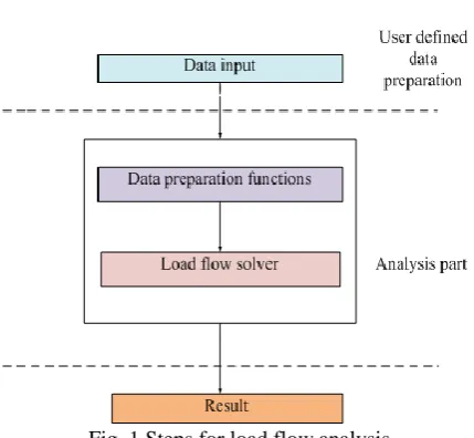
Fig. 1 Steps for load flow analysis
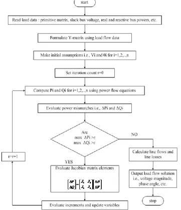
Newton Raphson method is the best opted method for solving non-linear load flow equations [5]. The number of iterations involved in Newton Raphson method is independent of number of buses considered, hence power flow equations can be solved just in few iterations. Keeping in view all these advantages, Newton Raphson method is popularly used for load flow studies in a power system [6]. In using Newton Raphson method, a direct solver is used to solve the linear systems. Basically an iterative technique is used in this method for obtaining optimal power flow solution.
Mathematical model for NR method
In application of the NR method, we have to first bring the equations to be solved, to the form f(x1, x2...) =0 where x1,
x2…xn are the unknown variables to be determined. Let us assume that the power system has 1 n PV buses and 2 n PQ
buses. In polar coordinates the unknown variables to be determined are:
(i) θi, the angle of the complex bus voltage at bus i, at all the PV and PQ buses. This gives us n1+n2 unknown
variables to be determined.
(ii) Vi, the voltage magnitude of bus i, at all the PQ buses. This gives us 2 n unknown variables to be determined.
Therefore the total number of variables to be computed is n1+2n2, for which n1+2n2 consistent equations needs to be
solved. The equations are as under;
∆𝑃𝑖 = 𝑃𝑖,𝑠𝑝𝑒𝑐 .− 𝑃𝑖,𝑐𝑎𝑙 .= 0 ∆𝑄𝑖 = 𝑄𝑖,𝑠𝑝𝑒𝑐 .− 𝑄𝑖,𝑐𝑎𝑙 .= 0
Where Pi,spec.= Specified active power at bus i Qi,spec.= Specified reactive power at bus i
Pi, cal. = Calculated value of active power using voltage estimates. Qi, cal .= Calculated value of reactive power using voltage estimates ΔP = Active power residue
ΔQ = Reactive power residue
Using polar coordinate system, the voltage magnitude equation, the real and reactive power equations can be expressed as:
Vi∗= Vi(cos θ + j sin θ)
Pi= Vi Vj(Gijcos θij+ Bij n
j=1
sin θij)
Qi = Vi Vj n
j=1
(Gijcos θij− Gijsin θij)
The power flow equations can be expanded into Taylor series using Newton Raphson method as follows:
∆P
∆Q = −J ∆θ ∆V V ∆P
∆Q = − H N K L
∆θ VD−1∆V ∆P
∆Q = J1 J2 J3 J4
Where ∆P = ∆P1 ∆P2 . . ∆Pn−1 ∆Q = ∆Q1 ∆Q2 . . ∆Qm ∆θ = ∆θ1 ∆θ2 . . ∆θn−1 ∆V = ∆V1 ∆V2 . . ∆Vm
VD =
V1 . . . V2 . . . Vm
And
H is a (n − 1) × (n − 1) matrix, and its element isHij = ∂∆Pi
∂θj.
N is a (n − 1) × m matrix, and its element is Nij= Vj ∂∆Pi
∂Vj.
K is a m × (n − 1) matrix, and its element is Kij = ∂∆Qi
∂θj.
L is an m × m matrix, and its element is Lij = Vj ∂∆Qi
∂Vj.
These parameters are the defining one in forming Jacobian matrix and hence to perform load flow solution.
Calculation of P cal. and Q cal. :
The real and reactive powers can be calculated using the following equations;
𝑃𝑖,𝑐𝑎𝑙 .= 𝑃𝑖 = 𝑉𝑖 𝑛
𝑗 =1
𝑉𝑗 (𝐺𝑖𝑗cos 𝜃𝑖𝑗 + 𝐵𝑖𝑗sin 𝜃𝑖𝑗)
𝑃𝑖 = 𝐺𝑖𝑖 𝑉𝑖2 + 𝑉𝑖 𝑛
𝑗 =1
𝑄𝑖,𝑐𝑎𝑙 .= 𝑄𝑖 = 𝑉𝑖 𝑉𝑗 (𝐺𝑖𝑗 𝑛
𝑗 =1
sin 𝜃𝑖𝑗 − 𝐵𝑖𝑗cos 𝜃𝑖𝑗)
𝑄𝑖 = −𝐵𝑖𝑖 𝑉𝑖2 + 𝑉𝑖 𝑉𝑗 𝑛
𝑗 =1
(𝐺𝑖𝑗sin 𝜃𝑖𝑗 − 𝐵𝑖𝑗cos 𝜃𝑖𝑗)
The powers are computed at any (r+1)th iteration by using the voltages available from previous iteration. The elements of the Jacobian are found using the above equations as:
IEEE 57 bus system
The standard IEEE 57-bus system consists of 80 transmission lines; seven generators at buses 1, 2, 3, 6, 8, 9, 12; and 15 OLTC transformers. The reactive power sources are considered at bus no. 18, 25 and 53. Line data, bus data and the minimum and maximum limits on control variables and dependent variables have been adapted from official IEEE standards and values. The total system active and reactive power demands are 1250.8 p.u. and 336.4 p.u. on 100 MVA base. The voltages of all load bus and generator bus have been constrained within limits of 0.94 p.u. to 1.06 p.u.
II. LITERATURE SURVEY
Tan et al. (2013) presented a paper applying the Newton-Raphson method based on current injection into the case of distribution network. Firstly, the correction equations of these two methods have been derived and compared. The Jacobian matrix of the traditional Newton-Raphson must be recalculated in each iteration, while the Newton-Raphson method based on current injection only need recalculate the diagonal elements of its Jacobian matrix which mainly consists of admittance matrix’s elements. It reduces the computation and makes the programming easier as well. Based on these, their convergence properties have been derived. Both of them have the quadratic convergence; the only difference is the coefficients. IEEE11bus system has been used to test this method, and compared with the traditional Newton-Raphson method. The results show the Newton-Raphson (N-R) method based on current injection reliable and effectively. The distribution network IEEE11 case shows that with the same initial values, the current injection methods can convergent to the upper part of the PV curve, that is the stable solution of the system. The IEEE11 case indicates the current injection method is more reliable than the traditional Newton-Raphson [8].
Wang et al. (2012) extended research on use of Newton Raphson method for load flow studies. The traditional methods, such as electricity method, the RMS current method and so on, in the calculation in the process of line loss is very dependent on load output curve of stationary condition. But power grid operation process load curve are changing. Therefore, use common method to calculate the line loss there is greater error. However, use improved Newton's method for grid loss calculation, because the data collection process of fully considering load change. The method to calculate the power loss results more close to the statistical energy loss, so that can effectively control the size of management energy loss. Therefore, this method can be used as a new method of distribution energy loss calculation [9].
Bijwe et al. (2003) presents new non divergent constant Jacobian Newton power flow methods. Both coupled and decoupled Jacobian versions have been developed. The non divergence feature of these methods is achieved through application of optimal multiplier theory for step size adjustment control. In order to verify the effectiveness of these methods results for four IEEE test systems, two Indian power systems and a famous 11-bus ill-conditioned distribution system have been obtained and compared with those obtained with the corresponding versions of the conventional power flows [10].
II.
METHODOLOGYIn present study, load flow study of IEEE 57 bus system has been done using Newton Raphson load flow algorithm. The MATPOWER software has been used to run the algorithm. To perform load flow analysis using Newton Raphson load flow method, the algorithm developed is as follows:
To perform load flow analysis using Newton Raphson method, the algorithm developed is as follows: Step 1: Form the nodal admittance matrix (Yij).
Step 2: Assume an initial set of bus voltage and set bus n as the reference bus as:
Vi= Vi, spec.∠00 (at all PV buses)
Vi= 1∠00 (at all PQ buses)
Step 3: Calculate the real Power Pi using the load flow equation;
2
1
cos
sin
n
i ii i i j ij ij ij ij j
P
G V
V V
G
B
Step 4: Calculate the reactive PowerQi using the load flow equation;
2
1
sin
cos
n
i ii i i j ij ij ij ij
j
Q
B V
V V
G
B
Step 5: Form the Jacobian matrix using sub-matrices H, N K and L. Step 6: Find the power differences ΔPiand Δ Qifor all i=1, 2, 3… (n-1);
∆𝑃𝑖 = 𝑃𝑖,𝑠𝑝𝑒𝑐 .− 𝑃𝑖,𝑐𝑎𝑙 . ∆𝑄𝑖 = 𝑄𝑖,𝑠𝑝𝑒𝑐 .− 𝑄𝑖,𝑐𝑎𝑙 .
Step 8: Stop the iteration if all ΔPi and ΔQi are within the tolerance values.
Step 9: Update the values of Vi and δi using the equation xk+1=xk+ Δxk.
In context to various steps involved in carrying out load flow studies with Newton Raphson method, following detailed flow chart has been designed:
Fig. 3 Detailed flow chart of Newton Raphson load flow method.
III.RESULTS AND DISCUSSION
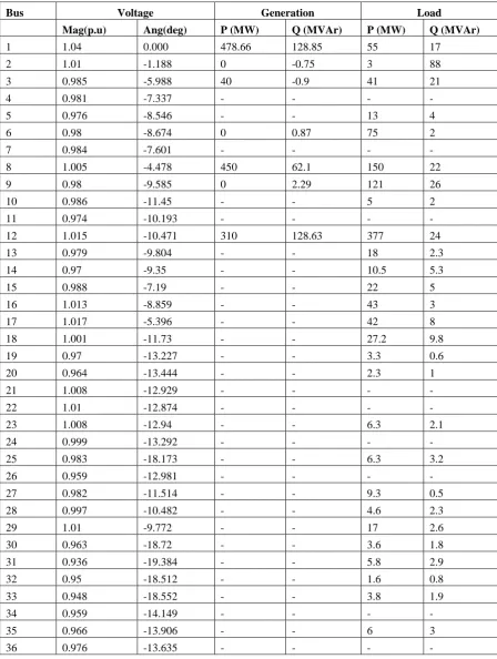
Table 1 Load flow results for IEEE 57-bus system using N-R method
Bus Voltage Generation Load
Mag(p.u) Ang(deg) P (MW) Q (MVAr) P (MW) Q (MVAr)
37 0.985 -13.446 - - - - 38 1.013 -12.735 - - 14 7 39 0.983 -13.491 - - - - 40 0.973 -13.658 - - - - 41 0.996 -14.077 - - 6.3 3 42 0.967 -15.533 - - 7.1 4.4 43 1.01 -11.354 - - 2 1 44 1.017 -11.856 - - 12 1.8 45 1.036 -9.27 - - - - 46 1.06 -11.116 - - - - 47 1.033 -12.512 - - 29.7 11.6 48 1.027 -12.611 - - - - 49 1.036 -12.936 - - 18 8.5 50 1.023 -13.413 - - 21 10.5 51 1.052 -12.533 - - 18 5.3 52 0.98 -11.498 - - 4.9 2.2 53 0.971 -12.253 - - 20 10 54 0.996 -11.71 - - 4.1 1.4 55 1.031 -10.801 - - 6.8 3.4 56 0.968 -16.065 - - 7.6 2.2 57 0.965 -16.584 - - 6.7 2
Total: 1278.66 321.08 1250.8 336.4 Various load flow losses can also be computed using N-R method which is tabulated as below:
Load flow losses for IEEE 57 bus system using N-R method
Branch From To From Bus Injection To Bus Injection Power loss
Bus Bus P (MW) Q (MVAr) P (MW)
Q
(MVAr) P (MW) Q (MVAr)
53 22 38 -10.73 -3.51 10.76 3.54 0.024 0.04 54 11 41 9.19 3.53 -9.19 -2.83 0 0.7 55 41 42 8.88 3.27 -8.69 -2.95 0.187 0.32 56 41 43 -11.59 -2.95 11.59 3.55 0 0.59 57 38 44 -24.35 5.23 24.52 -5.08 0.175 0.35 58 15 45 37.33 -0.73 -37.33 2.09 0 1.36 59 14 46 47.89 27.4 -47.89 -25.4 0 1.93 60 46 47 47.89 25.47 -47.29 -24.0 0.604 1.79 61 47 48 17.59 12.43 -17.51 -12.3 0.079 0.1 62 48 49 0.08 -7.38 -0.04 6.93 0.04 0.06 63 49 50 9.66 4.43 -9.58 -4.3 0.084 0.13 64 50 51 -11.42 -6.2 11.64 6.56 0.224 0.35 65 10 51 29.64 12.51 -29.64 -11.8 0 0.66 66 13 49 32.43 33.8 -32.43 -30.3 0 3.5 67 29 52 17.92 2.55 -17.45 -1.95 0.463 0.6 68 52 53 12.55 -0.25 -12.43 0.41 0.125 0.16 69 53 54 -7.57 -4.47 7.72 4.66 0.154 0.19 70 54 55 -11.82 -6.06 12.13 6.46 0.308 0.4 71 11 43 13.59 4.85 -13.59 -4.55 0 0.31 72 44 45 -36.52 3.28 37.33 -2.09 0.812 1.62 73 40 56 3.46 4.07 -3.46 -3.74 0 0.33 74 56 41 -5.43 0.66 5.61 -0.49 0.176 0.18 75 56 42 -1.58 1.46 1.59 -1.45 0.01 0.02 76 39 57 3.85 2.92 -3.85 -2.61 0 0.31 77 57 56 -2.85 0.61 2.86 -0.58 0.016 0.02 78 38 49 -4.66 -10.53 4.8 10.44 0.145 0.22 79 38 48 -17.22 -19.39 17.43 19.71 0.205 0.32 80 9 55 18.93 10.38 -18.93 -9.86 0 0.52 Total: 27.864 121.67
V. CONCLUSION
In this paper, an IEEE 57 based bus system for power flow is being discussed. In this experiment Newton Raphson method is studied and discussed to evaluate the load flow conditions including power losses for this bus system. This technique is studied using MATPOWER simulation software and the results showed faster convergence with reliable results.
REFERENCES
[1] Zian W. and Alvarado F. L., “Interval arithmetic in power flow analysis”, IEEE Transactions on Power System, Vol. 7, no. 3, pp. 1341-1349, 1992.
[2] Garcia P. A. N., Pereira J. L. R., Carneiro S., Vander M. da C., and Martins N., “Three-Phase Power Flow Calculations Using the Current
Injection Method”, IEEE Transactions on Power Systems, vol. 15, pp.508-514, 2000.
[4] Ambriz P., H., “Advanced SVC models for Newton-Raphson load flow and Newton optimal power flow studies,” IEEE Transactions on Power Apparatus and Systems, vol. 15, pp. 129-136, 2002.
[5] Stagg G. and El-Abiad A., Computer Methods in Power System Analysis, Tata McGraw-Hill, New York, 1968. [6] Heydt G., Computer Analysis Methods for Power Systems, Macmillan Publishing, New York, 1986.
[7] Panosyan A. and Oswald B., “Modified Newton-Raphson load flow analysis for integrated AC/DC power systems," in Proc. Universities Power Engineering Conference, UPEC 2004, vol. 3, pp. 1223-1227, 2004.
[8] Tan T., Li Y., Li Y., and Jiang T., “The Analysis of the Convergence of Newton-Raphson Method Based on the Current Injection in Distribution Network Case,” in Proc. International Journal of Computer and Electrical Engineering, vol. 5, pp. 288-290, 2013.
[9] Xiao ming Wang and Zhang Li, “Improved Newton’s Method for Calculation of Power Distribution Network Theory Energy Loss,” in proc. 2nd International Conference on Computer and Information Application, vol.6, pp. 1716-1718, 2012.
![Fig. 2 Single-line diagram of the IEEE 57 bus test system [7].](https://thumb-us.123doks.com/thumbv2/123dok_us/7782720.1286253/4.595.124.472.359.711/fig-single-line-diagram-ieee-bus-test.webp)