THE FINITE ELEMENT METHOD

(1)

F

THE FINITE ELEMENT METHOD

INTRODUCTION

Finite element methods are now widely used to solve structural, fluid, and multiphysics problems numerically (1). The methods are used extensively because engineers and scientists can mathematically model and numerically solve very complex problems. The analyses in engineering are performed to assess designs, and the analyses in the various scientific fields are carried out largely to obtain insight into and ideally to predict natural phenomena. The prediction of how a design will perform and whether and how a natural phenomenon will occur is of much value: Designs can be made safer and more cost effective, while insight into and the prediction of nature can help, for example, to prevent disasters. Thus, the use of the finite element method greatly enriches our lives.

As with many other important scientific developments, it is difficult to give an exact date of the ‘‘invention’’ of the finite element method. Indeed, we could trace back the development of the method to the Greek philosophers and in modern times to physicists, mathematicians, and engineers (see the discussions in Refs. 2 and 3). However, the real impetus for the development of what is now referred to as the finite element method was provided by the need to analyze complex structures in aeronautical engineering and the availability of the electronic computer. Namely, when using the finite element method, large sys-tems of algebraic equations need to be assembled and solved, and the computer provides the necessary means to accomplish this task.

The papers of Argyris and Kelsey (4) and Turner et al. (5) were seminal contributions in the 1950s. The name ‘‘finite element method’’ was coined by R.W. Clough in 1960 (6). The potential of the finite element method for engineering analysis was clearly foreseen, and henceforth the research on finite element methods started to accelerate in various research centers in Europe and in the United States. While significant papers and books were written in the next decade (see for example the references in Refs. 2 and 3), the development and rapidly increasing use of some com-puter programs clearly contributed in a major way to the acceptance and advancement of the method. Indeed, with no computer programs ever developed, the finite element method would have been a theoretical entity without much attention given to it.

The three finite element programs that had a major impact were ASKA, NASTRAN, and SAP (7–9). The NASTRAN and ASKA programs rapidly became major analysis tools in the aerospace and automotive industries. The SAP programs were largely used in civil and mechan-ical engineering industries and at universities. The avail-ability and wide use of the source codes of SAP IV and NONSAP with the description of the techniques used therein, see Bathe et al. (9–12), had a seminal effect on

the development of new algorithms, many finite element programs, and also finite element theory (3,13).

Today, finite element methods probably are used for the analysis of every major engineering design and probably in every branch of scientific studies. The method is now used primarily through the application of commercial finite element programs (see the section titled, ‘‘The Use of the Finite Element Method in Computer-Aided Engineer-ing’’). These programs are used on mainframes, worksta-tions and PCs and are employed to solve very complex problems. While the finite element methods were used originally for the analysis of solids and structures, the procedures are now employed also for the analysis of multi-physics problems, including fluid flows with fluid–struc-ture interactions (1–3).

The objective in the following sections is to briefly describe the finite element method and give some refer-ences that can be consulted for additional study. The description and references, of course, are by no means exhaustive. For the equations used, the notation of Ref. 3 is employed.

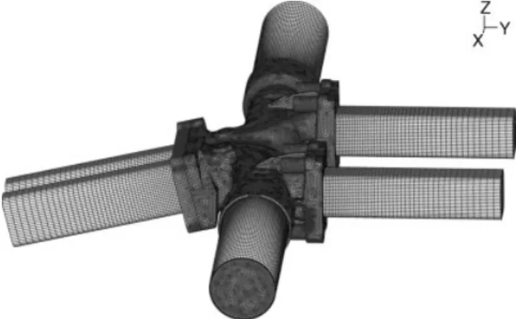
THE FORMULATION OF THE FINITE ELEMENT METHOD Figures 1 to 3 show typical finite element meshes (or finite element assemblages) modeling some solid, structural, and fluid systems. In each case the finite elements are used to represent the volume of the system. The finite elements are connected at the nodal points located at the corners and along the sides and in the faces of the elements. However, nodal points can also be located within the volume of an element. An important feature is that the finite elements do not overlap geometrically but together fill the complete volume of the solid or fluid.

Considering the analysis of a three-dimensional solid, like the wheel in Fig. 1, the geometry and the displacements of each element (within each element including all element surfaces) are completely described by the geometric posi-tions and displacements of the element nodal points. The element nodal coordinates prior to any displacements are known, of course, and the nodal displacements are the unknowns to be calculated. The basic step is to inter-polate the element geometry and the element displace-ments by using the nodal values. Here the isoparametric element interpolation, a most important development due to Irons (14), is largely used. For an element withqnodal points we use x¼X q i¼1 hixi; y¼ Xq i¼1 hiyi; z¼ Xq i¼1 hizi u¼X q i¼1 hiui; v¼ Xq i¼1 hivi; w¼ Xq i¼1 hiwi ð1Þ 1

Wiley Encyclopedia of Computer Science and Engineering, edited by Benjamin Wah. Copyright#_{2008 John Wiley & Sons, Inc.}

(2)

where thehiare the given interpolation functions, (xi,yi,zi)

are the known coordinates of nodal pointi, and (ui,vi,wi) are

the unknown displacements of nodal pointi. Thehi are

functions of the element natural coordinates(r, s, t), which relate uniquely to the global coordinates. In this assump-tion, the same interpolation is employed for the geometry and the displacements, and these equations are applicable to very general curved element configurations. However, in by far most analyses and certainly in nonlinear analy-ses, low-order linear, non-curved elements are preferred (4-node quadrilateral elements in the two-dimensional (2-D) analyses of solids, and 8-node brick elements in the three-dimensional (3-D) analyses of solids), but quadratic elements (9-node elements in 2-D analyses and 27-node elements in 3-D analyses) can be more effective (3). To obtain a more accurate solution, mostly the number of elements is simply increased; that is, the h-method is used. Alterna-tively, also the number and size of elements can be kept constant and the order of the geometry and displacement interpolations is increased; that is, the p-method is used. Of course, these approaches can also be combined and then an h/p-method is employed (15).

While some of the first finite elements for structural analyses were largely formulated based on physical insight and intuition, the development and use of a general theory based on the principle of virtual work (or virtual displacements) established a firm foundation and a general approach for the formulation of finite elements.

Today, the principle of virtual displacements is the basic equation used to formulate displacement-based finite ele-ments. Considering a general solid, this principle can be written as (3) Z V eTtdV¼ Z Sf uSfT_fSf_dS_þ Z V uTfBdV ð2Þ

where the unknown (real) stresses are t, the known applied body forces are fB, the known applied surface tractions are fSf_{, the virtual displacements are} _{u, and} the virtual strains that correspond to the virtual displace-ments aree. Of course, the stresses need to satisfy the given stress-strain laws, and the strains (the virtual and real quantities) must satisfy the strain–displacement relationships. Also, the real displacements must satisfy the given displacement boundary conditions and the vir-tual displacements must be zero at the locations of the prescribed real displacements. The integrations are per-formed over the volume,V, and traction-loaded surface, Sf, of the solid considered.

The principle of virtual displacements, with these con-ditions satisfied, is totally equivalent to the differential formulation of the boundary value problem. The principle is referred to also as a variational formulation and a weak formulation (2,3).

In linear analysis, the displacements are assumed to be infinitesimally small, the material laws are assumed to be constant, and the volume and surfaces over which the integrations are performed are known and constant, that is, unaffected by the displacements. Substituting from Equa-tion (1) into EquaEqua-tion (2) and invoking the principle of virtual displacements as many times as there are nodal displacement degrees of freedom, we obtain

KU¼R ð3Þ

whereKis the stiffness matrix,Uis the displacement vector listing all unknown nodal point displacements (theui,vi,wi,

for all nodes,i= 1, 2,. . ., as applicable), andRis a vector of externally applied forces at the nodal-point displacement Figure 1. Finite element model of a wheel using

three-dimensional brick elements, and a typical 8-node brick element (q=8).

Figure 2. Finite element model of a car body using predomi-nantly shell elements.

Figure 3. Finite element computational fluid dynamics (CFD) model of a manifold; FCBI elements, about 10 million equations solved in less than 1 hour on a single-processor PC.

(3)

degrees of freedom. The solution of Equation (3) yields the nodal displacements for Equation (1) and hence the strains and stresses in all elements.

In dynamic analysis, the body forces include inertia and damping effects, and these can be included directly in the solution to obtain (3)

M ¨UþCU

:

þKU¼R ð4Þ whereMis the mass matrix (usually a consistent mass matrix),Cis a damping matrix (frequently the Rayleigh damping matrix is used), and _U,¨ _U

:

_{denote the nodal} accelerations and velocities, respectively. In structural vibration analyses, these dynamic equilibrium equations are solved by using mode superposition or implicit direct time integration (for example, by using the popular tra-pezoidal rule).

However, for wave propagation analyses, the dynamic equilibrium equations solved are generally (3)

M ¨U¼RF ð5Þ whereFrepresents the nodal forces that correspond to the element stresses. Usually, a lumped (diagonal) mass matrix is used.

The above equations have been written for a three-dimensional solid, but also are applicable with appropri-ate modifications for the analysis of two-dimensional solids. Furthermore, the equations can be extended and then also are applicable for the analysis of structures modeled by beams, plates, and shells. The extension is reached by introducing midsurfaces, displacements and rotations, and the applicable kinematic and stress assumptions. For example, in the analysis of shells, the Reissner–Mindlin kinematic assumption—that plane sec-tions originally plane and normal to the midsurface of the shell remain plane—is introduced, and the assumption that the stress normal to that midsurface is zero is imposed. Because the pure displacement-based finite ele-ments are not effective for thin shells (and plates and beams), that is, they ‘lock’ in bending actions (see the section below titled, ‘‘The Analysis of Shells’’), mixed and hybrid formulations are used to reach more effective elements. The construction of such elements in essence is based on an extension of the principle of virtual displace-ments, namely the use of the Hu–Washizu variational principle (2,3). Effective structural elements can then directly be employed in Equations (3–5) together with the displacement-based solid elements (but of courseU now also includes nodal rotations).

Considering nonlinear analysis, the nonlinear effects can arise from nonlinear material behavior, like plasticity and creep; from geometric nonlinear effects, that is, large dis-placements and large strains; and from contact between bodies established as a result of the displacements. In these cases, the basic principle of virtual displacements and the extensions for structural elements still are directly applic-able, but the appropriate stress and strain measures need be used and the equilibrium need be considered in the deformed geometry of the bodies. For such general

non-linear analyses, the total Lagrangian (TL) and the updated Lagrangian (UL) formulations provide a fundamental basis of solution (3,16) and are widely used. In these formulations, the nonlinear material behavior is introduced to establish the stresses for ‘‘given’’ deformations, that is, not using a rate formulation when the constitutive relations are rate-independent (see also Ref. 17). If required, contact condi-tions including frictional effects are imposed as constraints on the nodal displacements and forces over the contacting surfaces. Because the large deformations and nonlinear material conditions and the solution for the actual areas of contact introduce significant nonlinearities in the govern-ing equations, iteration for solution in general is required (see below).

Considering a dynamic solution based on implicit direct time integration, and assuming that contact conditions are not present, the incremental nonlinear analysis is accom-plished by solving at discrete timesDtapart

MtþDtU¨ þCtþDtU

:

þtþDtF¼tþDtR ð6Þ where the equilibrium is considered at timetþDt, and the nodal forces tþDt_F _and tþDt_R _{correspond to the internal}

element stresses and the externally applied loads, respec-tively. In static analysis, simply the inertia and damping effects are neglected and the superscriptt¼time denotes the load level (but is also an actual physical variable when a material law is time-dependent).

Because the nodal forces highly depend on the deforma-tions and all the considered nonlinearities need be included in calculating these forces, an iteration is necessary for the solution of Equation (6). A Newton–Raphson iteration, or variant thereof, is commonly performed, with the govern-ing equations

tþDt_^

Kði1ÞDUðiÞ¼tþDtR^ði1ÞtþDtFði1Þ

tþDt_UðiÞ_¼tþDt_Uði1Þ_þ_D_UðiÞ ð7Þ

wheretþDt_K^ði1Þ _{is the effective tangent stiffness matrix} that corresponds to the linearization of the nodal force vectors with respect to the incremental displacements

DUðiÞ. The hat intþDt_K^ði1Þ_andtþDt_R^ði1Þ_{is used to signify}

that also mass and damping effects are included (3). In static analysis these effects of course are neglected. The iteration is continued until appropriate convergence cri-teria (based on forces, displacements, or energy) are satis-fied. To reach fast convergence, and quadratic convergence when near the solution, it is important to use the linear-ization ‘‘consistent’’ with the stress integration procedures and the force updating used to evaluate the right-hand side of Equation (7) (3,17,18).

If contact conditions are to be included, then for exam-ple, for normal contact the following conditions need be satisfied (3):

(4)

wheretþDt_g _{represents the gap and}tþDt_l _{represents the}

normal contact force. To reach stable and accurate solu-tions, appropriate interpolations of contact tractions need be used (19). Of course, with the relations in Equation (8) imposed as conditions on Equation (6), penetration is pre-vented at the contacting surfaces. Frictional contact con-ditions are similarly solved for; see Ref. 3. These concon-ditions to enforce contact between bodies enter into the iteration for equilibrium and compatibility; that is, Equation (7) needs to be amended to enforce the contact relations.

The use of Equation (7) (in general amended for contact conditions) for dynamic analysis of course implies that a transient solution with implicit time integration is pur-sued. If a short time duration or wave propagation analysis is to be performed (e.g., a crash simulation in the motor car industry), then an explicit time integration frequently is more effective. In this case, Equation (5), also amended to include contact conditions, is used with the nodal vectors continuously updated for all nonlinearities, which result from large deformations, contact and nonlinear material effects in the step-by-step solution. The solution is attrac-tive because no iteration is performed like in Equation (7); however, the disadvantage is that the time step size in the forward integration needs to be very small (because the time integration is only conditionally stable) (3).

Equations (7) and (5), as discussed above, are applicable to the nonlinear analysis of solids and structures; however, for structural elements, a mixed formulation need be used (see the section titled, ‘‘The Analysis of Shells’’). Also, in material nonlinear analysis, frequently (almost) incom-pressible conditions are encountered, as when modeling a rubber-like material or elasto-plastic conditions. In these cases, considering a solid, it is effective to use a mixed formulation in which the unknown displacements and pressure are interpolated; that is, the u/p formulation is employed (see the section titled, ‘‘The Reliable and Effective Analysis of Solids’’).

The same basic approach also can be followed to establish finite element solutions of heat transfer pro-blems (considering solids or fluids) and of incompressible fluid flows. In these cases, the temperature and the velocities (and pressure) need to be interpolated; in essence the ‘‘principle of virtual temperatures’’ and the ‘‘principle of virtual velocities’’ are employed. These prin-ciples in concept are similar to the principle of virtual displacements and hence of course also correspond to weak formulations. A major added difficulty arises in the use of the Eulerian formulation of fluid flows because of the convective effects. A pure interpolation of velocities and temperature results in a unstable solution. This instability can be circumvented, like in finite difference solutions, by introducing some form of upwinding (see the section titled, ‘‘Finite Element Discretizations for Incompressible Fluid Flows’’).

The Lagrangian formulations for the solids and struc-tures and the Eulerian formulations for fluid flows have been fully coupled by the use of arbitrary Lagangian– Eulerian formulations, referred to as ALE formulations for fluid–structure interactions. Such formulations are now used to solve reliably very complex multiphysics

problems that involve displacements of solids and struc-tures, temperature distributions, fluid flows, electromag-netic effects, and so on (see for example Refs. 1–3, and 20). EFFECTIVE FINITE ELEMENT PROCEDURES

The first requirement of any analysis is of course the selection of an appropriate mathematical model to repre-sent the physical problem (3). The next requirement is to solve this model with reliable and effective numerical methods. Because the use of reliable and effective finite element methods is very important, much research effort has been expended to reach such procedures.

The Reliable and Effective Analysis of Solids

The analysis of solids is efficiently accomplished by using the pure displacement-based finite element method referred to above, unless incompressible or almost incom-pressible material conditions are considered, as in the analysis of rubber-like materials or in elasto-plastic response. In incompressible analysis, the pure displace-ment-based discretizations ‘‘lock,’’ and a mixed interpola-tion based on displacements and pressure is much more effective. However, the appropriate combination of displa-cement and pressure interpolations must be used.

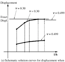
The phenomenon of locking is of fundamental impor-tance for the understanding of what we mean by a reliable finite element formulation. Figure 4 shows schematically the error in some norm between the finite element solution, uh, and the exact solution,u, of the mathematical model to

be solved, as the mesh is refined. Of course, the exact solution is in general not known, but we can think of a close approximation to the exact solution, obtained by a finite element analysis using a very fine mesh. If for almost incompressible analysis, a pure displacement-based finite element formulation is used, then the convergence curves in Figs. 4(a) and 4(b) are generally much below and above the respective curves obtained in the compressible analy-sis. Hence the error obtained for a given mesh depends on the bulk modulus and significantly increases as incompres-sible conditions are approached. Because the displace-ments become small measured on what they should be, the phenomenon is referred to as ‘‘locking’’. Finite element discretizations that lock, like schematically referred to in Fig. 4, are not reliable because small changes in some data can cause large changes in the solution error.

Hence a reliable finite element discretization displays the following convergence behavior in the appropriate norm:

kuuhk’chk ð9Þ

where c is a constant (that is, independent of the bulk modulus),his the generic element size, andkis the order of interpolation used. To reach such finite element discre-tizations in almost, or fully, incompressible analysis, the use of the displacement–pressure interpolation is effective where the displacement and pressure interpolations used should satisfy two conditions (3,21–23). First, the ellipticity

(5)

condition must be satisfied

aðv_h;v_hÞ akv_hk2 8v_h2K_hð0Þ ð10Þ where a (., .) is the (deviatoric strain energy) bilinear form of the problem, K_hð0Þ represents all those finite element interpolationsvhover the mesh which satisfy the

discre-tized zero divergence condition, andais a constant greater than zero. And second, the inf-sup condition should be satisfied for any mesh, and in particular ash!0,

inf

qh2Qh sup

vh2Vh R

VolqhdivvhdVol kvhkkqhk

b>0 ð11Þ

where, for the mesh,Vhis the space of displacement

inter-polations,Qhis the space of pressure interpolation,

appro-priate norms are used, andbis a constant. Effective finite elements that satisfy these two conditions are given, for

example, in Refs. 3 and 22. It is also possible to develop finite elements that bypass the inf-sup condition and do not lock, but these then depend on nonphysical numerical parameters (22,23).

The Analysis of Shells

The first developments of practical finite element methods were directed toward the analysis of aeronautical struc-tures, that is, thin shell structures. Since these first developments, much further effort has been expended to reach more general, reliable, and effective shell finite element schemes. Shells are difficult to analyze because they exhibit a variety of behaviors and can be very sensi-tive structures, depending on the curvatures, the thick-ness t, the span L, the boundary conditions, and the loading applied (23). A shell may carry the loading largely by membrane stresses, largely by bending stresses, or by combined membrane and bending actions. Shells that only carry loading by membrane stresses can be efficiently analyzed by using a displacement-based formulation (referred to above); however, such formulations ‘‘lock’’ (like discussed above when considering incompressible analysis) when used in the analysis of shells subjected to bending. To establish generally reliable and effective shell finite elements (that can be used for any shell ana-lysis problem), the major difficulty has been to overcome the ‘‘locking’’ of discretizations, which can be severe when thin shells are considered.

The principles summarized above for incompressible analysis apply, in essence, also in the analysis of plate and shell structures. The critical parameter is now the thick-ness to span ratio, t/L, and the relevant inf-sup expression ideally should be independent of this parameter. To obtain effective elements, the mixed interpolation of displace-ments and strain components has been proposed and is widely used in mixed-interpolated tensorial component (MITC) and related elements (3,23–25). The appropriate interpolations for the displacements and strains have been chosen carefully for the shell elements and are tied at specific element points. The resulting elements then only have displacements and rotations as nodal degrees of freedom, just as for the pure displacement-based elements. The effectiveness of the elements can be tested numerically to see whether the consistency, ellipticity, and inf-sup conditions (23) are satisfied. How-ever, the inf-sup condition for plate and shell elements is much more complex to evaluate than for incompressible analysis (26), and the direct testing by solving appropri-ately chosen test problems is more straightforward (23,27,28). Some effective mixed-interpolated shell ele-ments are given in Refs. 3,23 and 25.

For plates and shells, instead of imposing the Reiss-ner–Mindlin kinematic assumption and the assumption of ‘‘zero stress normal to the midsurface,’’ also three-dimensional solid elements without these assumptions can be used (29–31). Of course, for these elements to be effective, they also need to be formulated to avoid ‘‘lock-ing;’’ that is, they also need to satisfy the conditions mentioned above and more (23).

Figure 4. Locking phenomenon (when using pure displacement interpolations in almost incompressible analysis).

(6)

Finite Element Discretizations for Incompressible Fluid Flows Consideringallfluid flow problems, in engineering prac-tice most problems are solved by using finite volume and finite difference methods. Various CFD computer pro-grams based on finite volume methods are in wide use for high-speed compressible and incompressible fluid flows. However, much research effort has been expended on the development of finite element methods, in parti-cular for incompressible flows. Considering such flows and an Eulerian formulation, stable finite element procedures need to use velocity and pressure interpolations like those used in the analysis of incompressible solids (but of course velocities are interpolated instead of displacements) and also need to circumvent any instability that arises in the discretization of the convective terms. This requirement is usually achieved by using some form of upwinding (see for example Refs. 3, 32 and the references therein). However, another difficulty is that the traditional finite element formulations do not satisfy ‘‘local’’ mass and momentum conservation. Because numerical solutions of incompres-sible fluid flows in engineering practice should satisfy conservation locally, the usual finite element methods have been extended (see for example Ref. 33).

One simple approach that meets these requirements is given by the flow-condition-based interpolation (FCBI) formulation, in which finite element velocity and pressure interpolations are used to satisfy the inf-sup condition for incompressible analysis, flow-condition-dependent interpolations are used to reach stability in the convective terms, and control volumes are employed for integrations, like in finite volume methods (34). Hence stability is reached by the use of appropriate velocity and pressure interpolations, the conservation laws are satis-fied locally, and, also, the given interpolations can be used to establish consistent Jacobian matrices for the Newton– Raphson type iterations to solve the governing algebraic equations (which correspond to the nodal conditions to be satisfied).

An important point is that the FCBI schemes of fluid flow solution can be used directly to solve ‘‘fully coupled’’ fluid flows with structural interactions (20,35). The coupling of arbitrary discretizations of structures and fluids in which the structures might undergo large deformations is achieved by satisfying the applicable fluid–structure inter-face force and displacement conditions (20). The complete set of interface relations is included in the governing nodal point equations to be solved. Depending on the problem and in particular the number of unknown nodal point variables, it may be most effective to solve the governing equations by using partitioning (36). However, once the iterations have converged (to a reasonable tolerance), the solution of the problem has been obtained irrespective of whether parti-tioning of the coefficient matrix has been used.

While the solution of fluid–structure interactions is encountered in many applications, the analysis of even more general and complex multiphysics problems includ-ing thermo-mechanical, electromagnetic, and chemical effects is also being pursued, and the same fundamental principles apply (1).

Solution of Algebraic Equations

The finite element analysis of complex systems usually requires the solution of a large number of algebraic equa-tions; to accomplish this solution effectively is an important requirement.

Consider that no parallel processing is used. In static analysis, ‘‘direct sparse solvers’’ based on Gauss elimina-tion are effective up to about one half of a million equaelimina-tions for three-dimensional solid models and up to about 3 million equations for shell models. The essence of these solvers is that first graph theory is used to identify an optimal sequence to eliminate variables and then the actual Gauss elimination (that is, the factorization of the stiffness matrix and solution of the unknown nodal variables) is performed. For larger systems, iterative solvers possibly combined with a direct sparse solver become effective, and here in particular an algebraic multigrid solver is attractive. Mul-tigrid solvers can be very efficient in the solution of struc-tural equations but frequently are embedded in particular structural idealizations only (like for the analysis of plates). An ‘‘algebraic’’ multigrid solver in principle can be used for any structural idealization because it operates directly on the given coefficient matrix (37). Figure 5 shows a model solved by using an iterative scheme and gives a typical solution time.

Considering transient analysis, it is necessary to distin-guish between vibration analyses and wave propagation solutions. For the linear analysis of vibration problems, mode superposition is commonly performed (3,38). In such cases, frequencies and mode shapes of the finite element models need be computed, and this is commonly achieved using the Bathe subspace iteration method or the Lanczos method (3).

For the nonlinear analysis of vibration problems, usually a step-by-step direct time integration solution is performed with an implicit integration technique, and fre-quently the trapezoidal rule is used (3). However, when large deformation problems and relatively long time dura-tions are considered, the scheme in Ref. 39 can be much

Figure 5. Model of a rear axle; about a quarter of a million elements, including contact solved in about 20 minutes on a single-processor PC.

(7)

more effective. The solution of a finite element model of one half of a million equations solved with a few hundred time steps would be considered a large problem.

Of course, the explicit solution procedures already men-tioned above are used for short duration transient and wave propagation analyses (3,40).

In the simulations of fluid flows, the number of nodal unknowns usually is very large, and iterative methods need to be used for solution. Here algebraic multigrid solvers are very effective, but important requirements are that both the computation time and amount of memory used should increase about linearly with the number of nodal unknowns to be solved for. Figure 3 gives a typical solution time for a Navier–Stokes fluid flow problem. It is seen that with rather moderate hardware capabilities large systems can be solved.

Of course, these solution times are given merely to indicate some current state-of-the-art capabilities, and have been obtained using ADINA (41). Naturally, the solution times would be much smaller if parallel processing were used (and then would depend on the number of processors used, etc.) and surely will be much reduced over the years to come.

The given observations hold also of course for the solu-tion of multiphysics problems.

MESHING

A finite element analysis of any physical problem requires that a mesh of finite elements be generated. Because the generation of finite element meshes is a fundamental step and can require significant human and computational effort, procedures have been developed and implemented that automatize the mesh generation without human inter-vention as much as possible.

Some basic problems in automatic mesh generation are (1) that the given geometries can be complex with very small features (small holes, chamfers, etc.) embedded in otherwise rather large geometric domains, (2) that the use of certain element types is much preferable over other element types (for example, brick elements are more effec-tive than tetrahedral elements), (3) that graded meshes need be used for effective solutions (that is, the mesh should be finer in regions of stress concentrations and in boundary layers in fluid flows or the analysis of shells), and (4) that an anisotropic mesh may be required. In addition, any valu-able mesh generation technique in a general purpose ana-lysis environment (like used in CAE solution packages, see the section titled, ‘‘The Use of the Finite Element Method in Computer-Aided Engineering’’) must be able to mesh com-plex and general domains.

The accuracy of the finite element analysis results, measured on the exact solution of the mathematical model, highly depends on the use of an appropriate mesh, and this holds true in particular when coarse meshes need be used to reduce the computer time employed for complex analyses. Hence, effective mesh generation procedures are most important.

Various mesh generation techniques are in use (42). Generally, these techniques can be classified into mapped

meshing procedures, in which the user defines and con-trols the element spacings to obtain a relatively struc-tured mesh, and free-form meshing procedures, in which the user defines the minimum and maximum sizes of elements in certain regions but mostly has little control as to what mesh is generated, and the user obtains an unstructured mesh. Of course, in each case the user also defines for what elements the mesh is to be generated. Mapped meshing techniques in general can be used only for rather regular structural and fluid domains and require some human effort to prepare the input but usually result in effective meshes, in the sense that the accuracy of solution is high for the number of elements used. The free-form meshing techniques in principle can mesh automatically any 3-D domain provided tetrahedral elements are used; however, a rather unstructured mesh that contains many elements may be reached. The challenge in the development of free-form meshing procedures has been to reach meshes that in general do not contain highly distorted elements (long, thin sliver elements must be avoided unless mesh anisotropy is needed), that do not contain too many elements, and that contain brick elements rather than tetrahedral ele-ments. Two fundamental approaches have been pursued and refined, namely methods based on advancing front methodologies that generate elements from the boundary inwards and methods based on Delaunay triangulariza-tions that directly mesh from coarse to fine over the complete domain. Although a large effort has already been expended on the development of effective mesh generation schemes, improvements still are much desired, for example to reach more general and effective procedures to mesh arbitrary three-dimensional geome-tries with brick elements.

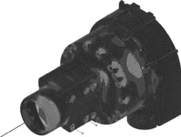
Figure 1 shows a three-dimensional mapped mesh of brick elements, a largely structured mesh, for the analysis of a wheel, and Fig. 6 shows a three-dimensional mesh of tetrahedral elements, an unstructured mesh, for the ana-lysis of a helmet. It is important to be able to achieve the grading in elements shown in Fig. 6 because the potential area of contact on the helmet requires a fine mesh.

Figure 7 shows another important meshing feature for finite element analysis, namely the possibility to glue in a ‘‘consistent manner’’ totally different meshes together (19). This feature provides flexibility in meshing different parts and allows multiscale analysis. The glueing of course is applicable in all linear and nonlinear analyses.

Because the effective meshing of complex domains still is requiring significant human and computational effort, some new discretization methods that do not require a mesh in the traditional sense have been developed (43). These techniques are referred to as meshless or meshfree methods but of course still require nodal points, with nodal point variables that are used to interpolate solid displace-ments, fluid velocities, temperatures, or any other conti-nuum variable. The major difference from traditional finite element methods is that in meshfree methods, the discrete domains, over which the interpolations take place, usually overlap, whereas in the traditional finite element methods, the finite element discrete domains abut each other, and geometric overlapping is not allowed. These meshfree

(8)

methods require appropriate nodal point spacing, and the numerical integration is more expensive (43,44). However, the use of these procedures coupled with traditional finite elements shows promise in regions where either traditional finite elements are difficult to generate or such elements become highly distorted in geometric nonlinear analysis (43).

THE USE OF THE FINITE ELEMENT METHOD IN COMPUTER-AIDED ENGINEERING

The finite element method would not have become a suc-cessful tool to solve complex physical problems if the method had not been implemented in computer programs. The success of the method is clearly due to the effective implementation in computer programs and the possible

wide use of these programs in many industries and research environments. Hence, reliable and effective finite element methods were needed that could be trusted to perform well in general analysis conditions as mentioned above. But also, the computer programs had to be easy to use. Indeed, the ease of use is very important for a finite element program to be used in engineering environments. The ease of use of a finite element program is dependent on the availability of effective pre- and post-processing tools based on graphical user interfaces for input and output of data. The pre-processing embodies the use of geometries from computer-aided design (CAD) programs or the construction of geometries with CAD-like tools, and the automatic generation of elements, nodal data, bound-ary conditions, material data, and applied loadings. An important ingredient is the display of the geometry and constructed finite element model with the elements, nodes, and so on. The post-processing is used to list and graphically display the computed results, such as the displacements, velocities, stresses, forces, and so on. In the post-processing phase, the computed results usually are looked at first to see whether the results make sense (because, for example, by an input error, a different than intended finite element model may have been solved), and then the results are studied in depth. In particular, the results should give the answers to the questions that provided the stimulus for performing the finite element analysis in the first instance.

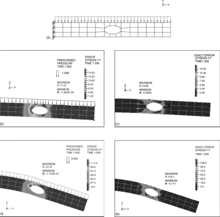
The use of finite element programs in computer-aided engineering (CAE) frequently requires that geometries from CAD programs need be employed. Hence, interfaces to import these geometries into the finite element pre-proces-sing programs are important. However, frequently the com-puter-aided design geometry can not be used directly to generate finite element meshes and needs to be changed (‘‘cleaned-up’’) to ensure well-connected domains, and by deleting unnecessary details. The effective importing of computer-aided design data is a most important step for the wide use of finite element analysis in engineering design. As mentioned already, the purpose of a finite element analysis is to solve a mathematical model. Hence, in the post-processing phase, the user of a finite element program ideally would be able to ascertain that a sufficiently accu-rate solution has been obtained. This means that, ideally, a measure of the error between the computed solution and the ‘‘exact solution of the mathematical model’’ would be available. Because the exact solution is unknown, only estimates can be given. Some procedures for estimating the error are available (mostly in linear analysis) but need to be used with care (45,46), and in practice frequently the analysis is performed simply with a very fine mesh to ensure that a sufficiently accurate solution has been obtained. Figure 8 shows an example of error estimation. Here, the scheme proposed by Sussman and Bathe (47) is used in a linear, nonlinear, and FSI solution using ADINA. In the first decades of finite element analysis, many finite element programs were available and used. However, the ensuing strive for improved procedures in these pro-grams, in terms of generality, effectiveness, and ease of use, required a significant continuous development effort. The resulting competition in the field to further develop and Figure 6. Model of a bicycle helmet showing mesh gradation.

(9)

Figure 8. Error estimation example: analysis of a cantilever with a hole. (a) Mesh of 9-node elements used for analysis of cantilever (with boundary conditions). (b) Cantilever structure — linear analysis, estimated error in region of interest shown. (c) Cantilever structure — linear analysis, exact error in region of interest shown. (d) Cantilever structure — nonlinear analysis, estimated error in region of interest shown. (e) Cantilever structure — nonlinear analysis, exact error in region of interest shown. (f) Cantilever structure — FSI analysis, estimated error in region of interest shown. (g) Cantilever structure — FSI analysis, exact error in region of interest shown.

(10)

continuously support a finite element program reduced the number of finite element systems now widely used to only a few: MSC NASTRAN, NX NASTRAN, ANSYS, ABAQUS, ADINA, and MARC are the primary codes used for static and implicit dynamic analyses of structures, and LS-DYNA, RADIOSS, PAMCRASH are the primary codes used for explicit dynamic analyses. For multiphysics pro-blems, notably fluid–structure interactions, primarily ADINA and ANSYS are used.

CONCLUSIONS AND KEY CHALLENGES

Since the first publications on the practical use of the finite element method, the field of finite element analysis has exploded in terms of research activities and applications. Numerous references are given on the World Wide Web. The method is now applied in practically all areas of engineering and scientific analyses. Since some time, the finite element method and related techniques frequently are simply referred to as ‘‘methods in computational fluid and solid mechanics.’’

With all these achievements in place and the abundant applications of computational mechanics today, it is surely

of interest to ask, ‘‘What are the outstanding research and development tasks? What are the key challenges still in the field?’’ These questions are addressed in the prefaces of Ref. 1, see the 2003 and 2005 volumes.

Although much has been accomplished, still, many exciting research tasks exist in further developing finite element methods. These developments and the envisa-ged increased use of finite element methods not only will have a continuous and very beneficial impact on tradi-tional engineering endeavors but also will lead to great benefits in other areas such as in the medical and health sciences.

Specifically, the additional developments of finite ele-ment methods should not be directed only to the more effective analysis of single media but also must focus on the solution of multiphysics problems that involve fluids, solids, their interactions, and chemical and electromag-netic effects from the molecular to the macroscopic scales, including uncertainties in the given data, and should also be directed to reach more effective algorithms for the optimization of designs.

Based on these thoughts, we can identify at least eight key challenges for research and development in finite ele-ment methods and numerical methods in general; these Figure 8. (Continued)

(11)

challenges pertain to the more automatic solution of math-ematical models, to more effective and predictive numerical schemes for fluid flows, to mesh-free methods that are coupled with traditional finite element methods, to finite element methods for multiphysics problems and multiscale problems, to the more direct modeling of uncertainties in analysis data, to the analysis and optimization of complete lifecycles of designed structures and fluid systems, and finally, to providing effective education and educational tools for engineers and scientists to use the given analysis procedures in finite element programs correctly and to the full capabilities (1).

Hence, although the finite element method already is widely used, still, many exciting research and develop-ment efforts exist and will continue to exist for many years.

BIBLIOGRAPHY

1. K. J. Bathe, ed.,Computational Fluid and Solid Mechanics.

New York: Elsevier, 2001, 2003, 2005, 2007.

2. O. C. Zienkiewicz and R. L. Taylor,The Finite Element Method,

Vols. 1 and 2, 4th ed., New York: McGraw Hill, 1989, 1990.

3. K. J. Bathe,Finite Element Procedures. Englewood Cliffs, NJ:

Prentice Hall, 1996.

4. J. H. Argyris and S. Kelsey, Energy theorems and structural

analysis,Aircraft Engrg., Vols. 26 and 27, Oct. 1954 to May

1955.

5. M. J. Turner, R. W. Clough, H. C. Martin, and L. J. Topp,

Stiffness and deflection analysis of complex structures, J.

Aeronaut. Sci.,23: 805–823, 1956.

6. R. W. Clough, The finite element method in plane stress

analysis,Proc. 2nd ASCE Conference on Electronic

Computa-tion, Pittsburgh, PA, Sept. 1960, pp. 345–378.

7. J. H. Argyris, Continua and discontinua,Proc. Conference on

Matrix Methods in Structural Mechanics, Wright-Patterson A.F.B., Ohio, Oct. 1965, pp. 11–189.

8. R. H. MacNeal, A short history of NASTRAN,Finite Element

News, July 1979.

9. K. J. Bathe, E. L. Wilson, and F. E. Peterson, SAP IV —A Structural Analysis Program for Static and Dynamic Response of Linear Systems, Earthquake Engineering Research Center Report No. 73–11, University of California, Berkeley, June 1973, revised April 1974.

10. K. J. Bathe, E. L. Wilson, and R. Iding, NONSAP—A Structural Analysis Program for Static and Dynamic Response of Nonlinear Systems, Report UCSESM 74–3, Department of Civil Engineering, University of California, Berkeley, May 1974. 11. K. J. Bathe, H. Ozdemir, and E. L. Wilson, Static and Dynamic

Geometric and Material Nonlinear Analysis, Report UCSESM 74-4, Department of Civil Engineering, University of Califor-nia, Berkeley, May 1974.

12. K. J. Bathe and E. L. Wilson,Numerical Methods in Finite

Element Analysis. Englewood Cliffs, NJ: Prentice Hall, 1976. 13. J. Mackerle, FEM and BEM in the context of information

retrieval,Comput. Struct.,80: 1595–1604, 2002.

14. B. M. Irons, Engineering applications of numerical integration

in stiffness methods,AIAA J.,4: 2035–2037, 1966.

15. I. Babusˇka and T. Strouboulis,The Finite Element Method and

its Reliability. Oxford, UK: Oxford Press, 2001.

16. K. J. Bathe, E. Ramm, and E. L. Wilson, Finite element

for-mulations for large deformation dynamic analysis, Int. J.

Numer. Methods Eng.,9: 353–386, 1975.

17. F. J. Monta´ns and K. J. Bathe, Computational issues in large strain elasto-plasticity: an algorithm for mixed hardening and

plastic spin,Int. J. Numer. Methods Eng.,63: 159–196, 2005.

18. M. Kojic´ and K. J. Bathe,Inelastic Analysis of Solids and

Structures. Berlin: Springer, 2005.

19. N. El-Abbasi and K. J. Bathe, Stability and patch test perfor-mance of contact discretizations and a new solution algorithm,

Comput. Struct.,79: 1473–1486, 2001.

20. K. J. Bathe and H. Zhang, Finite element developments for

general fluid flows with structural interactions,Int. J. Numer.

Methods Eng.,60: 213–232, 2004.

21. F. Brezzi and K. J. Bathe, A discourse on the stability

condi-tions for mixed finite element formulacondi-tions,J. Comput.

Meth-ods Appl. Mechanics Eng.,82: 27–57, 1990.

22. F. Brezzi and M. Fortin,Mixed and Hybrid Finite Element

Methods. Berlin: Springer, 1991.

23. D. Chapelle and K. J. Bathe,The Finite Element Analysis of

Shells – Fundamentals. Berlin: Springer, 2003.

24. K. J. Bathe and E. N. Dvorkin, A formulation of general shell elements — The use of mixed interpolation of tensorial

com-ponents,Int. J. Numer. Methods Eng.,22: 697–722, 1986.

25. K. J. Bathe, A. Iosilevich and D. Chapelle, An evaluation of the

MITC shell elements,Comput. Struct.,75: 1–30, 2000.

26. K. J. Bathe, The inf-sup condition and its evaluation for mixed

finite element methods,Comput. Struct., 79: 243–252, 971,

2001.

27. D. Chapelle and K. J. Bathe, Fundamental considerations for

the finite element analysis of shell structures,Comput. Struct.,

66: no. 1, 19–36, 1998.

28. J. F. Hiller and K. J. Bathe, Measuring convergence of mixed finite element discretizations: An application to shell

struc-tures,Comput. Struct.,81: 639–654, 2003.

29. K. J. Bathe and E. L. Wilson, Thick shells, inStructural

Mechanics Computer Programs, W. Pilkey, K. Saczalski and H. Schaeffer, eds. Charlottesville: The University Press of Virginia, 1974.

30. M. Bischoff and E. Ramm, On the physical significance of higher order kinematic and static variables in a

three-dimen-sional shell formulation,Int. J. Solids Struct.,37: 6933–6960,

2000.

31. D. Chapelle, A. Ferent and K. J. Bathe, 3D-shell elements and

their underlying mathematical model,Math. Models & Methods

Appl. Sci.,14: 105–142, 2004.

32. J. Iannelli,Characteristics Finite Element Methods in

Compu-tational Fluid Dynamics. Berlin: Springer Verlag, 2006. 33. T. J. R. Hughes and G.N. Wells, Conservation properties for the

Galerkin and stabilised forms of the advection-diffusion and

incompressible Navier-Stokes equations,J. Comput. Methods

Appl. Mech. Eng.,194: 1141–1159, 2005, and Correction195: 1277–1278, 2006.

34. K. J. Bathe and H. Zhang, A flow-condition-based interpolation

finite element procedure for incompressible fluid flows,

Com-put. Struct.,80: 1267–1277, 2002.

35. K. J. Bathe and G. A. Ledezma, Benchmark problems for

incompressible fluid flows with structural interactions,

Com-put. Struct.,85: 628–644, 2007.

36. S. Rugonyi and K. J. Bathe, On the finite element analysis of

fluid flows fully coupled with structural interactions,Comput.

(12)

37. K. Stuben, A review of algebraic multigrid,J. Computat. Appl. Math.,128(1–2): 281–309, 2001.

38. J. W. Tedesco, W. G. McDougal, and C. A. Ross,Structural

Dynamics. Reading, MA: Addison-Wesley, 1999.

39. K. J. Bathe, Conserving energy and momentum in nonlinear

dynamics: a simple implicit time integration scheme,Comput.

Struct.,85: 437–445, 2007.

40. T. Belytschko and T.J.R. Hughes (eds),Computational

Meth-ods for Transient Analysis. New York: North Holland, 1983.

41. K. J. Bathe, ADINA System,Encycl. Math.,11: 33–35, 1997;