Principles and Methodologies for the Determination of Shelf Life in Foods

Principles and Methodologies

for the Determination of Shelf–Life in Foods

Antonio Valero

_{, Elena Carrasco}

_{and Rosa M}

_{García-Gimeno}

_{University of Cordoba}

_{Centro Tecnológico del Cárnico (TEICA)}

Spain

1. Introduction

The establishment of validated methodologies for the determination of food shelf-life is currently demanded by both food industries and Health Authorities at national and international scale. It is well known that most foods are perishable, since they are subjected to modifications in their structure, composition and properties during storage before consumption. These changes are of physico-chemical origin attributed to food composition together with the action of intrinsic and extrinsic environmental factors, and also microbiological, where spoilage flora play an important role. These modifications are “translated into“ sensorial deterioration at a specific time point. In this respect, food-borne bacteria, despite representing a threat for consumers´ health, do not affect sensorial changes. Product “shelf-life” is defined, according to the American Heritage Dictionary of the English Language (Mifflin, 2006) as “the term or period during which a stored commodity remains effective, useful, or suitable for consumption”. But, which is understood by “unsuitable”? Mifflin (2006) defines “unsuitability” as “the quality of having the wrong properties for a specific purpose”. To know which is wrong and which is fine is not a straightforward question to answer, and often is subjected to individual perceptions. This issue is discussed later. Anyway, whichever the method to detect the unsuitability of a food product, once it is detected and established, its cause should be sought. Among the different elements which constitute and characterize a food product, generally only one is the responsible for the unsuitability of a product, namely, “the specific cause of unsuitability”. With this, going back to the definition of shelf-life, we could redefine “product shelf-life” in the food field as “the term or period a product may be stored before a specific element of the product makes it unsuitable for use or consumption”. This element could be of biological or physico-chemical nature.

In the last years, different procedures have been reported for the establishment of shelf-life, mainly based on the detection of microbial alteration, as well as physico-chemical and sensorial changes. The traditional approach consists of setting a cut-off point along the storage period at the time when any of the measured attributes exceeds a pre-established limit. Experimental work usually includes the storage of food product at different temperatures, performance of microbial analysis and the assesssment of spoilage by

sensorial testing. In the case of foods whose shelf-lives might be conditioned by the presence and proliferation of pathogenic microorganisms, experiments also involve challenge testing with the target organism prior to storage. The cut-off point has been traditionally referred as quality limit (if deterioration of food is known to be produced by physico-chemical changes), or safety limit (if deteriorarion of food is due to the presence of nocive chemical substances and/or pathogenic microorganisms, parasites or virus at levels of concern). This method is usually labour-intensive and expensive.

Regarding microbiological proliferation of spoilage and/or pathogenic microorganisms, predictive microbiology is recognized as a reliable tool for providing an estimation of the course of the bacteria in the foods, and indirectly, provide an estimation of shelf-life of the product in the cases when the cause of food spoilage or unacceptability is known to be microbiological. Indeed, mathematical modelling is a science-based discipline which aims to explain a reality with a few variables, and whose applications have been extended beyond research as a real added-value industrial application (Brul et al., 2007; McMeekin et al., 2002; Peleg, 2006; McMeekin, 2007).

The main concept behind the application of predictive microbiology for the determination of shelf-life based on spoilage is the specific spoilage organisms (SSO), which are associated to sensorial changes and spoilage. As such, the end of shelf-life can be defined as the time needed for SSO to multiply from an initial contamination level to a spoilage level, or the time invested by SSO to produce a certain metabolite causing sensorial rejection (Koutsoumanis & Nychas, 2000). In the case of pathogens, challenge test protocols are available for the determination of kinetic parameters (named maximum growth rate [µmax]

and lag time [lag]) of Listeria monocytogenes in ready-to-eat foods (SANCO, 2008). In addition, European Regulation No. 2073/2005, recommends the performance of predictive microbiology studies in order to investigate compliance with the criteria throughout the shelf-life. In particular, this applies to ready-to-eat foods that are able to support the growth of L. monocytogenes and that may pose a L. monocytogenes risk for public health. In general, proliferation of pathogens for which absence is required although might be present in foods, growth/no growth models are generally accepted as useful tools for the determination of the probability of growth, whereas those pathogens for which hazardous levels (i.e. Bacillus cereus) or toxin-producing organisms (i.e. Staphylococcus aureus) have been set, growth kinetic models are more appropriate to estimate the time until reaching such levels.

Quality, in a very broad sense, means satisfaction of consumers´ expectations; in other words, quality experience delivered by a food should match quality expectations of a consumer (van Boekel, 2008). Quality aspects of foods, such as colour, nutrient content, chemical composition etc., are governed by biochemical reactions (oxidation, Maillard reactions, enzyme activity) together with physical changes (aggregation of proteins, coalescence, sedimentation etc.). As for microbials, there are kinetic models for quality attributes. However, these models only provide a representation of single biochemical reactions within a well-diluted ideal system; thus, they are not easily extrapolated to other more complex matrices like foods.

Sensory testing is designed to validate the length of time that a product will remain with the same “acceptable quality” level or presents “no changes in desired sensory characteristics” over the entire life of a product (IFTS, 1993; Kilcast & Subramaniam, 2000). Some product properties are difficult to measure objectively. Moreover, instrumental measurement alone

cannot indicate consumer acceptability or rejection. It is very important to ensure no changes in sensory properties of foods during their shelf-lives, since consumers pay for a unconsciously established set of desired sensory characteristics.

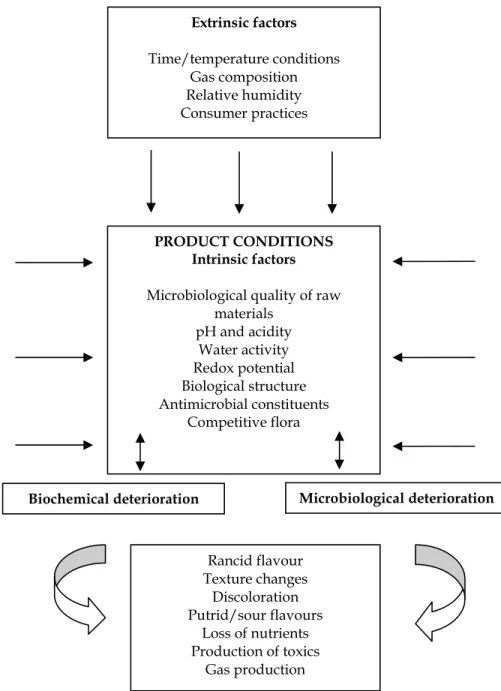
A unifying description of the interaction between microflora behaviour and physico-chemical changes undertaken in a food, represents a special challenge for food technologists. Such an integrated understanding of the interactions occurring during food storage should motivate the development of alternative preservation systems. A schematic representation of these phenomena is presented in Figure 1.

Throughout this chapter, the principles and methodologies for the establishment of shelf-life of foodstuffs are discussed. Also microbial, sensorial and physico-chemical parameters influencing shelf-life are analyzed. Subsequently, foods testing for data generation as well as procedures for assessment of shelf-life are reviewed. Finally, we will present some comments on future prospects.

2. Environmental factors affecting microbial shelf-life

Food spoilage is greatly influenced by environmental conditions concerning the food matrix, microbial characteristics, temperature, pH, water activity (aw), processing time, etc. The main

objective of studying the influence of environmental factors in food preservation is to inhibit spoilage due to microbial survival and growth and/or occurrence of chemical reactions. For this, a number of factors must be evaluated for different foods which could play an important role in the Hazard Analysis and of Critical Control Points (HACCP) system.

Regarding microbial growth, environmental conditions can affect largely the microbial load along the food chain. They can be classified as:

- Physical factors, such as temperature, food matrix. - Chemical factors, such as pH, preservatives, etc.

- Biological factors, such as competitive flora, production of metabolites or inhibiting compounds etc.

- Processing conditions affecting foods (slicing, mixing, removing, washing, shredding etc.) as well as influencing transfer of microorganisms (cross-contamination events). The application of one these factors alone can produce the desired effect on the food in terms of quality and safety, but this is not usual, especially in processed, ready-to-eat or perishable foods. Generally, the establishment of an adequate combination of more than one factor at moderate levels can offer the same result, but an improvement of the sensorial characteristics is achieved. This is the basic idea underlying the hurdle technology concept stated by Leistner (1995). Increasing the severity of one factor alone could produce a negative effect on food quality (e.g. chilling injury), while a moderate combination of several factors can lead to a shelf-life increase maintaining the original sensorial properties. For instance, in meat products, barriers such as the addition of salt, nitrite, modified atmosphere packaging, etc., can reduce the survival of pathogens (if present) and the proliferation of lactic acid bacteria during shelf-life.

2.1 Intrinsic factors

2.1.1 Microbiological quality of raw materials

Raw material entering the food industry represents a potential source of microbial contamination. The potential growth of pathogens and spoilage flora will be affected by the initial level of contamination and the efficacy of processing steps in eliminating bacteria in

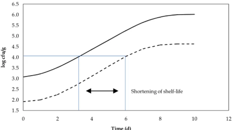
the food. Figure 2 represents the effect of various initial contamination levels on shelf-life of foods. At high contamination levels, less time would be needed by SSOs to reach the minimum spoilage level, thus, shelf-life would have to be reduced.

1.5 2.0 2.5 3.0 3.5 4.0 4.5 5.0 5.5 6.0 6.5 0 2 4 6 8 10 12 lo g c fu /g Time (d) Shortening of shelf-life

Fig. 2. Effect of the microbial initial contamination on shelf-life in a food.

A better raw material quality in terms of microbial contamination can be achieved by setting out a more strict suppliers control at primary production level, and optimizing sampling schemes. With an initial good quality of raw materials, processing operations, formulation of foods and storage conditions, shelf-life of foods could be extended.

2.1.2 pH and acidity

A widely used preservation method consists of increasing the acidity of foods either through fermentation processes or the addition of weak acids. The pH is a measure of the product acidity and is a function of the hydrogen ion concentration in the food product. It is well known that groups of microorganisms have pH optimum, minimum and maximum for growth in foods. Bacteria normally grow faster between pH ranges of 6.0 - 8.0, yeasts between 4.5 - 6.0 and moulds between 3.5 - 4.0.

An important characteristic of a food is its buffering capacity, i.e. its ability to resist changes in pH. Foods with a low buffering capacity will change pH quickly in response to acidic or alkaline compounds produced by microorganisms, whereas foods with high buffering capacity are more resistant to such changes. In any case, if low pH is a factor included in the preservation system of a food, control of pH and the application of a margin of safety are required for these foods.

2.1.3 Water activity (aw)

The requirements for moisture by microorganisms are expressed in terms of water activity (aw). The aw is therefore one of the most important properties of food governing microbial

growth and is defined as the free or available water in a food product (Fennema, 1996). Thus, the aw of a food describes the fraction of water “not bounded” to the components of a

food, i.e. the fraction of “available” water to participate in chemical/biochemical reactions and promote microbial survival and growth.

As for pH, control of aw and the application of a margin of safety are required for these food

products whose preservation system includes low aw. Microorganisms respond differently

to aw depending on a number of factors. These factors can modify the minimum and

maximum aw values to grow. Generally, Gram (-) bacteria are more sensitive to changes in

aw than Gram (+) bacteria. The growth of most foodborne pathogens is inhibited at aw

values below 0.86. 2.1.4 Redox potential (Eh)

The oxidation-reduction potential (Eh) of a food is the ease by which it gains or loses

electrons (Jay, 1992). The Eh value at which microorganisms will grow determines whether

they require oxygen (i.e. aerobic/microaerophilic environment) for growth or not (i.e. anaerobic environment). According to their Eh value, microorganisms can be classified into

the three following groups:

Aerobes +500 to +300 mV; Anaerobes +100 to -250 mV; and Facultative anaerobes +300 to -100 mV

Although Eh as inhibitory factor is especially important in meat products (Leistner, 2000),

product safety control should not solely focus on this factor since its measurement is subjected to limitations. Indeed, the Eh values are highly variable depending on the pH of

the food, extent of microbial growth, packaging conditions, oxygen partial pressure in the storage environment, and ingredients. Measurement requirements for Eh in foods are

reported by Morris (2000). 2.1.5 Biological structure

The natural surfaces of foods usually provide high protection against the entry and subsequent damage by spoilage organisms. External layers of seeds, the outer covering of fruits, and the eggshell are examples of biological protective structures. Several factors can influence the penetration of organisms through these barriers: (i) the maturity of plant foods enhances the effectiveness of the protective barriers; (ii) physical damage due to handling during harvest, transport, or storage, as well as invasion of insects can allow the penetration of microorganisms (Mossel et al., 1995); (iii) during the preparation of foods, processes such as slicing, chopping, grinding, and shucking destroy the physical barriers, thus favouring contamination inside the food.

Eggs can be seen as a good example of an effective biological structure that, when intact, will prevent external microbial contamination of the perishable yolk. Contamination by

Salmonella, one of the most prevalent contaminant, is possible through transovarian infection before this shell structure is established. Additional factor is the egg white and its antimicrobial components. When there are cracks through the inner membrane of the egg, microorganisms may further penetrate into the egg. Factors such as storage temperature, relative humidity, age of eggs, and level of surface contamination will influence the internalization of microorganisms.

2.1.6 Antimicrobial constituents

Food products may contain substances (i.e. antimicrobial constituents) which have antimicrobial properties against the growth of specific microorganisms. There is a wide variety of substances with recognized antimicrobial activity in a wide variety of food products. Other antimicrobial constituents in food products are added as preservatives. Some forms of food processing will also result in the formation of antimicrobial substances in food products including:

- Smoking, e.g. fish and meat products; - Fermentation, e.g. meat and dairy products;

- Condensation reactions between sugars and amino acids (i.e. Maillard reaction) during heating of certain foods.

2.1.7 Competitive flora (biopreservation)

Biopreservation techniques are the result of the development of a microorganism which may have an antagonistic effect on the microbial activity of other undesired microorganisms present in the food product (Mossel et al., 1995). There has been an increasing interest in biopreservation treatments in minimally processed foods in order to guarantee food safety whilst maintaining organoleptical properties.

Antagonistic processes include competition for essential nutrients, changes in pH value or Eh or the formation of antimicrobial substances like bacteriocins, which may negatively

affect the survival or growth of other microorganisms (Huis in’t Veld et al., 1996). Bacteriocins have been widely recognized as natural food biopreservatives, and latest advances on bacteriocin research have opened new fields to explore their role (García et al., 2010). The use of competitive microorganisms such as lactic acid bacteria against L. monocytogenes has been proven as a useful preservation technique in several food products (Brillet et al., 2005).

2.2 Extrinsic factors

2.2.1 Time/temperature conditions

All microorganisms have a defined temperature range within which they can grow. This range is limited by a minimum temperature needed for growth and a maximum temperature which does not support the growth. While the growth speed increases with increasing temperature, it tends to decline rapidly after the optimum temperature has been reached. An understanding of the interplay between time, temperature, and other intrinsic and extrinsic factors is crucial to select appropriate storage conditions for a food product. Temperature has a dramatic impact on the growth of microorganisms. Time plays an important role as a factor facilitating (long time) or avoiding (short time) the growth of microorganisms during food storage.

At low temperatures, two phenomena avoid microbial growth: - Intracellular reactions, which become much slower; and

- Fluidity of the cytoplasmic membrane, interfering with transport mechanisms (Mossel et al., 1995).

At temperatures above the maximum temperature, structural cell components become denatured and heat-sensitive enzymes are inactivated.

2.2.2 Gas composition

Many scientific studies have demonstrated the antimicrobial activity of gases at ambient and sub-ambient pressures in foods (Loss & Hotchkiss, 2002). The oxygen availability is related to the Eh and plays a role in product packaging, together with CO2 concentration. A variety

of common technologies are used to inhibit the growth of microorganisms, and a majority of these methods have shown high inhibitory effect when applied with low temperatures. Technologies include Modified Atmosphere Packaging (MAP), Controlled Atmosphere Packaging (CAP), Controlled Atmosphere Storage (CAS) or Direct Addition of Carbon Dioxide (DAC) (Loss & Hotchkiss, 2002).

An adequate packaging formulation in food products should extend shelf-life without affecting their sensorial properties. In general, the inhibitory effect of CO2 increases at low

temperatures due to the fact that solubility of CO2 becomes higher (Jay, 2000). Also, a

synergistic effect has been observed when CO2 has been applied together with low pH. The

major concern when extending the shelf-life of a product by MAP is that the inhibition of spoilage bacteria could allow the proliferation of foodborne pathogens as they do not compete for nutrients or physical space anymore, and consequently foods, in spite of presenting an acceptable sensorial quality, may be unsafe.

There are several additional intrinsic and extrinsic factors affecting the efficacy of antimicrobial atmospheres, such as product temperature, product-to-headspace gas volume ratio, initial microbial load, package barrier properties, biochemical composition of the food, etc. By combining antimicrobial atmospheres with other preservation techniques, further enhancement of food quality and safety can be achieved (Leistner, 2000).

2.2.3 Relative humidity (RH)

Relative humidity (RH) is the quantity of moisture in the atmosphere surrounding a food product whether packaged or not. It is calculated as a percentage of the humidity required to completely saturate the atmosphere (i.e. saturation humidity). Typically, there will be an exchange of moisture between a food product and the surrounding atmosphere which continues until the food reaches equilibrium.

The RH is closely related with aw and may actually alter the aw of a food. It is important to

assure that the product is stored with an environment where the RH prevents aw changes.

For example, if the aw of a food is set at 0.60 to assure its stability, it is important that this aw

value remains during storage by establishing adequate RH conditions so that the food does not pick up moisture from the ambient air. When foods with low RH values are placed in environments of high RH, they pick up moisture until equilibrium is established. Likewise, foods with high aw lose moisture when placed in an environment of low RH.

Determining the appropriate storage/packaging conditions for a food product is therefore essential for food safety and quality assurance. It is important to note that RH is related to temperature during storage (Esse & Humidipack, 2004).

2.2.4 Consumer practices

Consumer practices during dispatch, storage and use of food products in the home are obviously outside the control of food industries. However, food industries should take account of poor consumer handling in the establishment of product shelf-life, at least, those known to be popular. For example, many domestic refrigerators do not operate at refrigeration temperatures between 0-5ºC, being above this range; this can greatly affect the safety of food products and shorten their shelf-life (Carrasco et al., 2007). Food industries should wisely establish food shelf-lives according to real temperature records of domestic refrigerators, and not to theoretical refrigeration temperatures.

3. Role of spoilage microorganisms in foods

Foods are dynamic systems which experience changes in pH, atmosphere, nutrient composition and microflora over time. Each food product has its own unique flora, determined by the raw materials used, food processing parameters and subsequent storage conditions. The growth of SSOs in perishable foods is largely affected by several environmental factors already explained in the Section 2.

The main purpose of the application of one or a combination of intrinsic and extrinsic factors on a food product is to destroy and/or inhibit SSOs and pathogenic microorganisms, thus providing a more extended shelf-life, or to improve the sensorial characteristics of the food.

The microorganisms dominating a product can be predicted by understanding how the major preservation parameters affect microbial selection. The identification of SSOs are very important for the calculation of the remaining shelf-life of a given food product (Gram et al., 2002). Some examples are Lactobacillus sakei in cooked meat products (Devlieghere et al., 2001), Photobacterium phosphoreum, Shewanella spp and Pseudomonas spp in fishery products (Dalgaard et al., 1997; Gram and Dalgaard, 2002), Brochothrix thermosphacta in precooked chicken (Patsias et al., 2006), or gram negative bacteria in fresh-cut (Rico et al., 2007).

It is crucial to introduce quantitative considerations (Gram, 1989) since the spoilage activity of an organism is its quantitative ability to produce spoilage metabolites (Dalgaard, 1995; Dalgaard et al., 1993). In other words, it is necessary to evaluate if the levels of a particular organism reached in naturally spoiled foods are capable of producing the amount of metabolites associated with spoilage. In general, it requires a careful combination of microbiology, sensory analyses and chemistry to determine which microorganism(s) are the SSOs of a particular food product.

It is generally known that almost all microbial groups include species that could cause spoilage in a given food under specific conditions. Initially, different populations are present in a contaminated food, and some groups become more predominant after a certain storage period. This selection might depend on several physico-chemical factors (as discussed previously) and processing and storage conditions. For instance, in meat products stored at aerobic conditions, Pseudomonas spp. can produce metabolites and slime formation, but in an anaerobic atmosphere, the predominant SSOs are shift to lactic-acid bacteria, producing lactic acid and decreasing pH.

Vegetables are a special case due to the nutrient composition. The high pH (usually close to neutrality) will allow a range of Gram-negative bacteria to grow, but spoilage is specifically caused by organisms capable of degrading the vegetable polymer, pectin (Liao et al., 1997). These organisms, typically Erwinia spp. and Pseudomonas spp. are the SSO of several ready-to-eat vegetable products (Lund, 1992); also pectin degrading fungi can play a role in vegetable products (Pitt & Hocking, 1997). However, when decreasing pH due to the addition of organic acids in minimally processed fruits and vegetables, growth of fungi, yeasts and lactic-acid bacteria become the SSOs (Edwards et al., 1998).

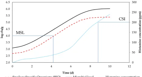
After identification of the SSOs and the range of environmental conditions under which a particular SSO is responsible for spoilage, the next step in microbial shelf-life establishment is the decision about the microbial level of SSO above which spoilage occurs and shelf-life ends (Dalgaard, 1995; Koutsoumanis & Nychas, 2000). This step often requires a good understanding of the microbial evolution as a function of time. Initially, SSO is present in low quantities and constitutes only a minor part of the natural microflora. During storage, SSO generally produce the metabolites responsible for off-odours, off-flavours slime and finally cause sensory rejection. The cell concentration of SSO at rejection may be called the Minimal Spoilage Level (MSL) and the concentration of metabolites corresponding to spoilage is named Chemical Spoilage Index (CSI) (Dalgaard, 1993).

An example of these concepts is presented in Figure 3. In this case, the evolution of SSO together with histamine content occurs during storage of a seafood product. If MSL is set at 4 log cfu/g (if this limit is proven to cause food spoilage), the established shelf-life would be 4.2 days. However, this limit is largely different if the results are based on the histamine content, because if CSI is set at 200 ppm, the life would be 8.8 days. Generally, shelf-life may be determined based on the parameter that firstly produces alteration, in this example, microbial growth.

0 50 100 150 200 250 300 2.0 2.5 3.0 3.5 4.0 4.5 5.0 5.5 6.0 6.5 0 2 4 6 8 10 12 H is ta m in e c o n ce n tr at io n ( p p m ) lo g c fu /g Time (d)

Spoilage Specific Organisms (SSO) Microbial load Histamine concentration

Fig. 3. Theoretical growth of SSO together with evolution of histamine content in a seafood product. MSL (Microbial Spoilage Level), CSI (Chemical Spoilage Index).

MSL

The limit of microbial growth that determines shelf-life differs according to the food type and storage conditions. SSO counts from 105 _{to 10}8 _{cfu/g are commonly considered as}

convenient quality limits. For microorganisms which produce toxins, 105 _{cfu/g has been}

established as a limit for risk management in processed foods (Rho & Schaffner, 2007). The time to reach hazardous levels by pathogens should determine the shelf-life limit. In these cases, shelf-life is greatly influenced by the initial contamination level. Thus, hygienic control measures must be taken in order to prevent their presence in raw material and processed food products.

Several studies relate limits for microbial groups defining the end of shelf-life with specific food products. In this sense, 107 _{cfu/g has been chosen for aerobic bacteria in minced chicken}

meat (Grandinson & Jennings, 1993), freshwater crayfish (Wang & Brown, 1983), or fresh-cut lettuce (Koseki & Ito, 2002). For other microbial groups such as coliforms in cottage cheese, yeasts in shredded chicory endive, or mesophilic bacteria in fresh-cut spinach, limit levels of 102_{, 10}5 _{or 10}8 _{cfu/g, respectively, have been proposed (Babic & Watada, 1996; Jacxsens et al.,}

2001; Mannheim & Soffer, 1996). To set these limits, a thorough knowledge about the particular microbial ecology and deterioration causes of foods during storage is required. In relation with the microbiological limits previously mentioned, Regulation (EC) No. 2073/2005 regarding microbiological criteria in foodstuffs sets out two groups of criteria: - Food safety criteria which define the acceptability of a product or a batch. They are

applicable to foodstuffs placed on the market and throughout the shelf-life of the food. - Process hygiene criteria which define the acceptability of the process. These apply only

during the manufacturing process.

Other microbiological criteria for the end of shelf-life have been suggested by International Guidelines in Ready-To-Eat (RTE) foods. Some guidance documents are mainly focused on the study of growth of L. monocytogenes (SANCO, 2008) while other more general reports assess the microbiological quality of RTE foods placed in the market (Health Protection Agency, 2009; Refrigerated Food Association, 2009) or recommend specific principles to food industries (Food Safety Authority of Ireland, 2005; New Zealand Food Safety Authority, 2005). All of them establish microbiological criteria by specifying numerical limits, or admissible log increases during shelf-life.

4. Mathematical modelling of bacterial growth

It is a goal of food microbiologists to know in advance the behavior of microorganisms in foods under foreseeable conditions. If it was possible to predict the growth/survival/ inactivation of a microorganisms at given fixed conditions, it would be possible to systematically establish a shelf-life based on bacterial behaviour. The development of mathematical models describing the behavior of microorganisms under established conditions satisfactorily fulfill the challenge proposed. Already in 1921, Bigelow (1921) described the logarithm nature of thermal death, but it was not until the 1980s when mathematical models for predicting bacterial behavior experienced a great development. A new field emerged in the food microbiology area: “predictive microbiology”, or as redefined recently, “modeling of microbial responses in foods”. McKellar & Lu (2004a) presented a detailed review of predictive models published so far. Since primary to tertiary models,

mathematical models have been extensively applied, in part due to the predictive friendly-software developed, where most models are implemented.

The advent of computer technology and associated advances in computational power have made possible to perform complex mathematical calculations that otherwise would be too time-consuming for useful applications in predictive microbiology (Tamplin et al., 2004). Computer software programs provide an interface between the underlying mathematics and the user, allowing model inputs to be entered and estimates to be observed through simplified graphical outputs. Behind predictive software programs are the raw data upon which the models are built. Some of the most popular software are: GInaFiT (Geeraerd, et al., 2005), where different inactivation models are available (http://cit.kuleuven.be/ biotec/ downloads.php); DMFit (Baranyi & Roberts, 1994), with implementation of a dynamic growth primary model (http://www.combase.cc/index.php/en/downloads/category/11-dmfit); Pathogen Modeling Program (Buchanan, 1993), which incorporates a variety of models of different pathogens in broth culture and foods (http://pmp.arserrc.gov/ PMPOnline.aspx); Seafood Spoilage and Safety Predictor (SSSP) (Dalgaard et al., 2002), offering models for specific spoilage microorganisms and also for L. monocytogenes in seafood (http://sssp.dtuaqua.dk/); ComBase (Baranyi & Tamplin, 2004), a predictive tool for important foodborne pathogenic and spoilage microorganisms (http:// www.combase.cc / index.php/en/predictive-models); Sym´Previus (Leporq et al., 2005), a tool with a collection of models and data to be applied in the food industry context, e.g. strengthening HACCP plans, developing new products, quantifying microbial behavior, determining shelf-lives and improving safety (http://www.symprevius.net/); Microbial Responses Viewer (Koseki, 2009), a new database consisting of microbial growth/no growth data derived from ComBase, and also modelling of the specific growth rate of microorganisms as a function of temperature, pH and aw (http:// mrv. nfri.

affrc.go.jp/Default.aspx#/About); Escherichia coli fermented meat model (Ross & Shadbolt, 2004), describing the rate of inactivation of Escherichia coli, due to low aw or pH or both, in

fermented meats (http://www.foodsafetycentre.com.au/fermenter.php).

In a further step, a number of software called expert systems have been developed to provide more complex decision support based on a set of rules and algorithms for inference based on the relationships underlying these rules. In these systems, the core knowledge is stored as a series of IF-THEN rules that connect diverse evidence such as user input, data from databases, and the formalized opinions of experts into a web of knowledge. There are various examples of decision-support systems which encapsulate knowledge that is based in predictive microbiology, such as those applied in predicting food safety and shelf-life (Witjes et al., 1998; Zwietering et al., 1992); a step-wise system structured as a standard risk assessment process to assist in decisions regarding microbiological food safety (van Gerwen et al., 2000); or other systems for microbial processes described by Voyer & McKellar (1993) and Schellekens et al. (1994).

Whiting & Buchanan (1994) called the above integrated software models-based “tertiary models”. They defined tertiary-level models as personal computer software packages that use the pertinent information from primary- and secondary-level models to generate desired graphs, predictions and comparisons. “Primary-level models” describe the change in microbial numbers over time, and “secondary-level models” indicate how the features of primary models change with respect to one or more environmental factors, such as pH,

temperature and aw. Below is a description of the most relevant primary and secondary

models, as well as their uses and scope. 4.1 Primary models

Primary models aim to describe the kinetics of the process (growth or survival or inactivation) with as few parameters as possible, while still being able to accurately define the distinct stages of the process.

In the context of foods shelf-life, the process observed depends on the group of microorganisms studied (e.g. total aerobic flora, lactic acid bacteria, Enterobacteriaceae, etc.) and the characteristics and storage conditions of foods (e.g. presence of antimicrobials like nitrites, aw, pH, temperature of storage, atmosphere inside the food package, etc.). Often,

different groups of microorganisms behave differently in the same food product. For example, in fermented meat products, it is usual to observe growth of lactic acid bacteria against the survival or inactivation of other bacteria groups (González & Díez, 2002; Moretti et al., 2004; Rubio et al., 2007).

The application of primary models to a set of microbiological data proceeds as follows. In a first step, a mathematical model is assumed to explain the data, that is, how microbial counts change over time. In a second step, such model is fitted to microbiological data by means of regression (linear or non-linear). As a consequence of the fitting process, estimates for a number of kinetics parameters embedded in the model is provided, for example, for the rate of growth/inactivation or lag time (in growth processes) or “shoulder” (in inactivation processes). The dataset used to fit the model is assumed to be obtained under specific intrinsic and extrinsic factors. For this reason, the kinetic parameters provided after fitting solely apply for the specific intrinsic and extrinsic factors characterizing the dataset. Several primary models have been published. Below is described the most important models used for growth and survival/inactivation.

4.1.1 Growth models

The first book devoted exclusively to the field of predictive microbiology (McMeekin et al., 1993) provide an excellent review and discussion of the classical sigmoid growth functions, especially the modified logistic and Gompertz equations. As they point out, these are empirical applications of the original logistic and Gompertz functions. Over the last years, a new generation of bacterial growth curve models have been developed that are purported to have a mechanistic basis: for example, the Baranyi model (Baranyi et al., 1993; Baranyi et al., 1994), the Hills model (Hills & Mackey, 1995; Hills & Wright, 1996), the Buchanan model (Buchanan et al., 1997), and the heterogeneous population model (McKellar, 1997).

a. Sigmoidal functions such as the modified logistic (Equation 1) and the modified Gompertz (Equation 2) introduced by Gibson et al. (1987), have been the most popular ones used to fit microbial growth data since these functions consist of four phases, similar to the microbial growth curve.

 





 









Logx t exp A C exp_ B t M _ (2) where x(t) is the number of cells at time t, A is the lower asymptotic value as t decreases to

zero, C is the difference between the upper and lower asymptote, M is the time at which the absolute growth rate is maximum, and B is the relative growth rate at M.

The parameters of the modified Gompertz equation (A, C, B and M) can be used to characterize bacterial growth as follows:

 









lag  M – 1 / B LogN 0  _  A / BC / e _ (3) specific growth rate BC / e »BC / 2.18 (4) In order to simplify the fitting process, reparameterized versions of the Gompertz equation

have been proposed (Zwietering et al., 1990; Willox et al., 1993):













10

Log x A Cexp exp 2.71 Rg/C t  1 (5) where A = log10 x0 (log10 cfu x ml-1), x0 is the initial cell number, C the asymptotic increase in

population density (log10 cfu x ml-1), Rg the growth rate (log10 cfu h-1), and is the lag-phase

duration (h).

Although used extensively, some authors (Whiting & Cygnarowicz-Provost, 1992; Baranyi, 1992; Dalgaard et al., 1994; Membré et al., 1999) reported that the Gompertz equation systematically overestimated growth rate compared with the usual definition of the maximum growth rate. Note that there is also no correspondence between the lower asymptote and the inoculum size x0. Baty et al. (2004), while comparing the ability of

different primary models to estimate lag time, found that the Gompertz model is perhaps the least consistent. Nevertheless, this model is one of the most widely used to fit bacterial curves, notably by the Pathogen Modeling Program (Buchanan, 1993).

b. Baranyi et al. (1993) and Baranyi & Roberts (1994, 1995) introduced a mechanistic model for bacterial growth (Equation 6). In this model, it is assumed that during lag phase, bacteria need to synthesize an unknown substrate q critical for growth. Once cells have adjusted to the environment, they grow exponentially until limited by restrictions dictated by the growth medium.

max max ( ) ( ) 1 ( ) ( ) 1 m q t dx x t x t dt q t  x  _{ }     _    _  _     (6)

where x is the number of cells at time t, xmax the maximum cell density, and q(t) is the concentration of limiting substrate, which changes with time (Equation 7). The parameter m

characterizes the curvature before the stationary phase. When m = 1 the function reduces to a logistic curve, a simplification of the model that is often assumed.

max ( )

dq

q t

The initial value of q (q0) is a measure of the initial physiological state of the cells. A more

stable transformation of q0 may be defined as:

0 max 0 1 ln 1 h q           (8)

Thus, the final model has four parameters: x0, the initial cell number; h0; xmax; and µmax. The

parameter h0 describes an interpretation of the lag first formalized by Robinson et al. (1998).

Using the terminology of Robinson et al (1998), h0 may be regarded as the “work to be done” by the bacterial cells to adapt to their new environment before commencing exponential growth at the rate, max, characteristic of the organism and the environment. The duration of the lag, however, also depends on the rate at which this work is done which is often assumed to be max.

c. Hills & Mackey (1995) and Hills & Wright (1996) developed a theory of spatially dependent bacterial growth in heterogeneous systems, in which the transport of nutrients was described by the combination a structured-cell kinetic model with reaction-diffusion equations. The total biomass in the culture M at a time t is dependent on time and a rate constant A (Equation 9), while the total number of cells in the culture

N depends on time and the rate constants A and Kn (Equation 10).

 

 

 

M t M At (9)

 

 

 



 



N t N _K At A K t _ A K (10)

The rate constants A and Kn depend on all the environment factors. The lag time and the doubling time have the following relationships:





 





This shows that if the rate constants A and Kn have similar activation energies, the ratio of lag to doubling time (tD) should be nearly independent of temperature. This model takes no account of possible lag behavior in the total biomass (M).

Hills model can also be generalized to spatially inhomogeneous systems such as food surfaces (Hills & Wright, 1996). If more detailed kinetic information on cell composition is available, more complex multicompartment kinetic schemes can be incorporated.

d. Buchanan et al. (1997) proposed a three-phase linear model. It can be described by three phases: lag phase, exponential growth phase and stationary phase, described as follows: Lag phase:

0

For ,ttLAG NtN (13)





For ,t_LAG t t_MAX N_tN  µ t t– _LAG (14) Stationary phase:

For ,ttMAX NtNMAX (15)

where Nt is the log of the population density at time t (log cfu ml-1); N0 the log of the initial

population density (log cfu ml-1_{); NMAX the log of the maximum population density}

supported by the environment (log cfu ml-1_{); t the elapsed time; tLAG the time when the lag}

phase ends (h); and µ is the maximum growth rate (log cfu ml-1 _h-1_).

In this model, the growth rate was always at maximum between the end of the lag phase and the start of the stationary phase. The µ was set to zero during both the lag and stationary phases. The lag was divided into two periods: a period for adaptation to the new environment (ta) and the time for generation of energy to produce biological components needed for cell replication (tm).

e. McKellar model assumes that bacterial population exists in two “compartments” or states: growing or nongrowing. All growth was assumed to originate from a small fraction of the total population of cells that are present in the growing compartment at t

= 0. Subsequent growth is based on the following logistic equation: 1 MAX dG G G dt  N          (16)

where G is the number of growing cells in the growing compartment. The majority of cells were considered not to contribute to growth, and remained in the nongrowing compartment, but were included in the total population. While this is an empirical model, it does account for the observation that growth in liquid culture is dominated by the first cells to begin growth, and that any cells that subsequently adapt to growth are of minimal importance (McKellar, 1997). The model derives from the theory that microbial populations are heterogeneous rather than homogeneous, existing two populations of cells that behave differently; the sum of the two populations effectively describes the transition from lag to exponential phase, and defines a new parameter G0, the initial population capable of

growing. Reparameterization of the model led to the finding that a relationship existed between µmax and as described in Baranyi model. In fact, Baranyi & Pin (2001) stated that

the initial physiological state of the whole population could reside in a small subpopulation. Thus, the McKellar model constitutes a simplified version of the Baranyi model, and has the same parameters.

The concept of heterogeneity in cell populations was extended further to the development of a combined discrete-continuous simulation model for microbial growth (McKellar & Knight, 2000). At the start of a growth simulation, all of the cells were assigned to the nongrowing compartment. A distribution of individual cell lag times was used to generate a series of discrete events in which each cell was transferred from nongrowing to the growing compartment at a time corresponding to the lag time for that cell. Once in the growing compartment, cells start growing immediately according to Equation 16. The combination of the discrete step with the continuous growth function accurately described the transition from lag to exponential phase.

At the present time it is not possible to select one growth model as the most appropriate representation of bacterial growth (McKellar & Lu, 2004b). If simple is better, then the three-phase model is probably sufficient to represent fundamental growth parameters accurately (Garthright, 1997). The development of more complex models (and subsequently more mechanistic models) will depend on an improved understanding of cell behavior at the physiological level.

4.1.2 Survival/inactivation models

Models to describe microbial death due to heating have been used since the 1920s, and constitute one of the earliest forms of predictive microbiology. Much of the early work centered on the need to achieve the destruction of Clostridium botulinum spores. This type of models has undertaken great advances from the classical linear inactivation model to others more sophisticated nonlinear models.

a. The classical linear model assumes that inactivation is explained by a simple first-order reaction kinetics under isothermal conditions (Equation 17):

t t

dS K S

dt    (17)

where St is the survival ratio (Nt/N0) and k´ is the rate constant. Thus the number of

surviving cells decreases exponentially:

k´t

e t

S   (18)

and when expressed as log10, gives:

logSt  kt (19)

where k = k´/ln 10. The well-known D-value (time required for a 1-log reduction) is thus equal to 1/k, where k is the slope. The D-value can also be expressed as:

0 log log t t D value N N   _ (20)

When log D-values are plotted against the corresponding temperatures, the reciprocal of the slope is equal to the z-value, which is the increase in temperature required for a 1-log decrease in D-value. The rate constant can also be related to the temperature by the Arrhenius equation: 0 a E RT k N e _       (21)

where Ea is the activation energy, R the universal gas constant, and T is the temperature in Kelvin degrees.

Extensive work has been performed to calculate D-values and the z-value for most pathogens in broth culture and different food matrices (Mazzota, 2001; Murphy et al., 2002; van Asselt & Zwietering, 2006).

b. Although the concept of logarithmic death is still applied, nonlinear curves have been reported for many years, i.e. curves exhibiting a “shoulder” region at the beginning of the inactivation curve and/or a “tail” region at the end of the inactivation curve. Stringer et al. (2000) summarized the possible explanations for this behavior. Some of them are the variability in heating procedure, the use of mixed cultures, clumping, protective effect of dead cells, multiple hit mechanisms, natural distribution of heat sensitivity or heat adaptation.

We now know that cells do not exist simply as alive or dead, but may also experience various degrees of injury or sublethal damage, which may give rise to apparent nonlinear survival curves (Stringer et al., 2000). Survival modeling should also include a more complete understanding of the molecular events underpinning microbial resistance to the environment.

As heterogeneity is the most plausible reason for observing nonlinearity, the use of distributions to account for this nonlinearity such as gamma (Takumi et al., 2006) or Weibull (Coroller et al., 2006; van Boekel, 2002) have been suggested; from these, Weibull is the favored approach at the moment.

Also, “mirror images” of the primary growth models described above have been used to explain the inactivation process, such as the “mirror image” of the logistic function (Cole et al., 1993; Pruitt et al., 1993; Whiting, 1993), the “mirror image” of the Gompertz function (Linton et al., 1995) and the “mirror image” of the Baranyi model (Koutsoumanis et al., 1999).

4.2 Secondary models

These models predict the changes in the parameters of primary models such as bacterial growth rate and lag time as a function of the intrinsic and extrinsic factors. A description of the most popular secondary models is provided below. Two different approaches can be distinguished: i) the effects of the environmental factors are described simultaneously through a polynomial function; this type of model has probably been the most extensively used within predictive microbiology; and ii) the environmental factors are individually modeled, and a general model describes the combined effects of the factors; this approach is notably applied in the development of the increasingly popular square root and cardinal parameter-type models.

4.2.1 Polynomial models

Polynomial models describe the growth responses ( max, lag) or their transformations (√( max), ln( max), …) through a polynomial function. An example of a polynomial model is that proposed by McClure et al. (1993) for Brochothrix thermosphacta:

max 0 1 2 3 4 5 2 2 2 2 6 7 7 8 9 ln( ) (% ) (% ) (% ) (% ) a a T a pH a NaCl a T pH a T NaCl a pH NaCl a T a T a pH a NaCl               (22)

Polynomial models allow in almost every case the development of a model describing the effect of any environmental factor including interactions between factors. Moreover, the fit of polynomial models does not require the use of advanced techniques such as the

non-linear regression. The disadvantages of polynomial models lie in the high number of parameters and their lack of biological significance.

4.2.2 Square root-type

Temperature was the first environmental factor taken into account in square root-type models. Based on the observation of a linear relationship between temperature and the square root of the bacterial growth rate in the suboptimal temperature range, Ratkowsky et al. (1982) proposed the following function:

max b T T( min)

   (23)

where b is a constant, T is the temperature and Tmin the theoretical minimum temperature for growth. This equation was extended to describe the effect of temperature in the entire temperature range allowing bacterial growth, the so-called ‘biokinetic range’ (Ratkowsky et al., 1983):













max b T T( min) 1 exp c T Tmax

     (24)

where Tmax is the theoretical maximum temperature for growth and c a model parameter without biological meaning. These models were extended to take into account other environmental factors such as pH and water activity. McMeekin et al. (1987) proposed the following equation to describe the combined effects of temperature (suboptimal range) and water activity on the growth rate of Staphylococcus xylosus:





max b T T( min) aw awmin

    (25)

where awmin is the theoretical minimum water activity for growth. More recently, square root models have also been expanded to include, for example, the effects of CO2, (Devlieghere et

al., 1998) or pH and lactic acid concentration (Presser et al., 1997; Ross et al., 2003). 4.2.3 The gamma concept and the cardinal parameter model

Zwietering et al. (1992) proposed a model called “Gamma model”, describing the growth rate relative to its maximum value at optimal conditions for growth:

 

 

 

max opt T pH aw

     (26)

where µopt is the growth rate at optimum conditions, and γ(T), γ(pH), γ(aw) are the relative effects of temperature, pH and aw, respectively. The concept underlying this model

(“Gamma concept”) is based on the following assumptions: i) the effect of any factor on the growth rate can be described, as a fraction of opt, using a function (γ) normalized between 0 (no growth) and 1 (optimum condition for growth); and ii) the environmental factors act independently on the bacterial growth rate. Consequently, the combined effects of the environmental factors can be obtained by multiplying the separate effects of each factor (see Equation 26). Ross & Dalgaard (2004) considered that while this apparently holds true for growth rate under conditions where growth is possible, environmental

factors do interact synergistically to govern the biokinetic ranges for each environmental factor.

At optimal conditions for growth, all γ terms are equal to 1 and therefore max is equal to opt. The γ terms proposed by Zwietering et al. (1992) for the normalized effects of temperature, pH and aw are given in Equations 16 to 18.

 

 

γ-type terms for pH and lactic acid effects on growth rate were also included in square root-type models by Presser et al. (1997) and Ross et al. (2003).

Introduced by Rosso et al. (1993, 1995), the cardinal parameter models (CPMs) were also developed according to the Gamma concept. The relative effects of temperature, pH and aw

on the bacterial growth rate are described by a general model called CPMn:

    



 



 







min min max min

max 0 , , 1 0 , n n

opt opt opt opt opt

X X X X X X CM X X X X X X X X X X X X n X X nX X X   _   _{ }         _        _     (30)

where X is temperature, pH or aw. Xmin and Xmax are respectively the values of X below and above which no growth occur. Xopt is the value of X at which bacterial growth is optimum. n is a shape parameter. As for the “Gamma model” of Zwietering et al. (1992), CMn(Xopt) is equal to 1, CMn(Xmin) and CMn(Xmax) are equal to 0.

For the effects of temperature and pH, n is set to 2 and 1 respectively (Augustin et al., 2000a, 2000b; Le Marc et al., 2002; Pouillot et al., 2003 Rosso et al., 1993, 1995). For the effects of aw,

n is set to 2 (Augustin et al., 2000a, 2000b; Rosso & Robinson, 2001). The combined effects of the environmental factors are also obtained by multiplying the relative effects of each factor. Thus, the Cardinal Parameter Model for the effects of temperature, pH and aw on max can be written as: max optCM T CM pH CM a2( ) 1( ) 2( w)   (31) or alternatively: max optCM T CM pH CM a2( ) 1( ) 1( w)   (32)

In many ways, CPMs resemble the square root model. Responses predicted by the two types of models can be almost identical (Oscar, 2002; Ross & Dalgaard, 2004; Rosso et al., 1993,

1995). The advantages of the CPMs lie in the lack of structural correlation between parameters and the biological significance of all parameters (Rosso et al., 1995).

Several attempts have been made to include in CPMs the effects of organic acids (Augustin et al., 2000a, 200b; Coroller et al., 2003; Le Marc et al., 2002) or other inhibitory substances (Augustin et al., 2000a, 200b).

4.2.4 Artificial neural networks

“Black boxes” such as artificial neural networks are an alternative to the models above and have been used to develop secondary growth (or lag time) models (Garcia-Gimeno et al, 2002, 2003, Geeraerd et al., 1998). For further details on the principles of this method in the context of predictive microbiology, consult Hajmeer et al. (1997), Hajmeer & Basher (2002, 2003).

4.2.5 Probabilistic models

Probabilistic growth/no growth models can be seen as a logic continuation of the kinetic growth models. If environmental conditions are getting more stressful, growth rate is decreasing until zero and lag phase is increasing until eternity or at least longer than the period of experimental data generation. At these conditions, the boundary between growth and no growth has been reached and the modeling needs to shift from a kinetic model to a probabilistic model. The output of a probabilistic model will be the chance that a certain event will take place within a certain given time under conditions specified by the user. The period of time is an important criterion, as evolving from ‘no growth’ to ‘growth’ is, in many cases, possible as long as the period of analysis is sufficiently extended.

In the case of probabilistic models, responses will be coded as either 0 (response not observed) or 1 (response observed), under a specific set of conditions. If replicate observations are performed at a specific condition, a probability between 0 and 100% will be obtained. To relate this probability to the predictor variables, logistic regression is used (McMeekin et al., 2000; Ratkowsky & Ross, 1995). The logit function is defined as:









LogitP log P/ 1 –P (33)

where P is the probability of the outcome of interest.

Logit P is commonly described as some function Y of the explanatory variables, i.e.:

LogitP Y (34)

Equation 34 can be rearranged to:









where Y is the function describing the effects of the independent variables.

Several works have reported the application of probability models to different pathogens and spoilage microorganisms in foods (Lanciotti et al., 2001; Membré et al., 2001; Stewart et al., 2001).

5. Chemical spoilage

Chemical spoilage is mainly characterized by flavour and colour changes due to oxidation, irradiation, lipolysis (rancid) and heat. These changes may be induced by light, metal ions or excessive heat during processing or storage. Chemical processes may also bring physical changes such as increased viscosity, gelation, sedimentation or color change.

Biochemical reactions during food storage are relevant for the appearance of sensorial defects. Some of them are summarized as follows (Van Boekel, 2008):

- Lipid oxidation can lead to a loss of essential fatty acids and presence of rancidity, mainly due to the presence of free fatty acids. This phenomenon is associated to enzymatic oxidation, lipolysis, and discoloration.

- Non enzymatic and enzymatic browning can affect color, taste and aroma, nutritive value, and can contribute to the formation of toxicologically suspect compounds (acrylamide).

- Hydrolysis, lipolysis and proteolysis can cause changes in flavor, texture, vitamin content and formation of bitter taste.

- Separation and gelation are physical phenomena associated to sedimentation, creaming, gel formation and texture changes.

The first two processes normally characterize the majority of chemical spoilage phenomena in foods, and are explained below.

5.1 Lipid oxidation

Lipid oxidation is one of the most common causes of deterioration of food quality. Unsaturated fats are oxidized by free radical autoxidation, a chain reaction process catalyzed by the products of the reaction. The susceptibility and the rate of oxidation increase as the number of double bonds in the fatty acid increases.

Foods containing fat, e.g. milk, can undergo a number of subtle chemical and physical changes caused by lipolysis. Lipolysis can be defined as the enzymatic hydrolysis of fats by lipases. The accumulation of the reaction products, especially free fatty acids is responsible for the common off-flavour, frequently referred to as rancidity.

Fat stabilization is based on the use of physical methods (controlling temperature and light conditions during storage) and addition of antioxidants. In this sense, many foods or food ingredients contain components which with antioxidant properties (King et al., 1993). Examples of well known natural antioxidants are ascorbic acid, vitamin E (tocopherols), carotenoids and flavonoids. Antioxidants inhibit lipid oxidation by acting as hydrogen or electron donors, and interfere with the radical chain reaction by forming non radical compounds.

5.2 Non enzymatic and enzymatic browning

Non enzymatic browning resides in various chemical reactions occurring during food processing and storage. It is related to the formation of brown compounds and volatile substances that influence the sensorial quality of foods. Non enzymatic browning is in part associated to Maillard reactions. These include a number of complex reactions that are influenced by a large variety of factors (substrates nature, time/temperature combinations, pH, aw, or presence of inhibitor compounds). Control and prevention measures of non

enzymatic browning are based on the elimination of substrates, control of physico-chemical factors (shortening time and temperature, lowering pH) or addition of inhibitors such as sulfites, which delay the presence of pigments by means of fixing intermediate reaction products. Likewise, sulfites act against enzymatic browning and growth of microorganisms. Thus, they are used as preservatives in grape juices, wine, dehydrated fruits and concentrated juices.

Non enzymatic browning is a quality parameter for many dehydrated foods. For other products such as baked goods, coffee, molasses, and some breakfast foods, browning is desirable. However, in other foods browning is undesirable, decreasing the value or quality of the product. The browning include: decreased nutritional value from protein loss, off-flavor development, undesirable color, decreased solubility, textural changes, destruction of vitamins and increased acidity (Franzen et al., 1990). Other effects are destruction of essential amino acids such as lysine, formation of mutagenic compounds and modifications in the antioxidant capacity of foods.

Enzymatic browning is defined as the enzymatic transformation, in presence of oxygen at first stage, from phenolic compounds to colored polymers. Dark pigments formed as result of these reactions are known as melanines. Enzymatic browning is produced in fruits vegetables, which are rich in phenolic compounds, normally after harvesting and during processing conditions (washing, peeling, chopping, etc.). Polyphenoloxidases (PPO) and peroxidases found in fruit tissues can catalyze the oxidation of certain endogenous phenolic compounds to quinones that polymerize to form intense brown pigments (Lewis & Shibamoto, 1986).

Since enzymatic browning can cause important losses in agriculture production, control and prevention of the principal mechanisms of these reactions are crucial. These methods are based on the activity against enzymes, substrates and/or product reactions. Their use might depend on the specific food to be considered, as well as other nutritional, technical, economical, sensorial or ethical considerations.

6. Sensorial evaluation for determining shelf-life

As stated previously, sensorial evaluation is an essential task for establishing shelf-life of food products. Once a food product is designed (composition, packaging, foreseeable conditions of storage and use, target population), next step consists of estimating the period of time during which the food maintains its original sensorial properties. An immediate question arises from the last assertion: “how could I assess that sensorial properties do not change along time?” In other words, “how can these differences be detected?”. There are different sensory tests to provide answer to this question; they are named sensory difference tests. However, at the same time, another question may come up to our minds: “Who should

detect these difference (in case they are detectable)?”. This is not a straightforward question to answer, as it greatly depends on the food quality management of the company. One could think that trained panellists are the most appropriate to detect possible differences in sensorial characteristics of foods during storage. After all, they are “sensorial instruments”. However, actually, they do not represent the target population, and probably, target population in general would not detect differences in such a perfect manner as trained panellists would do. So, it is very important to design an adequate test fitted to the needs, potential and politics of the company.

A sensory difference test allows for the possible distinction between various foods. In the case of the application of these tests to shelf-life estimation, a distinction should be made between the food under storage (at the foreseeable conditions) and the food just produced. The most common sensory difference tests are the paired-comparison test, the duo-trio test, and the triangle test (O´Mahony, 1985).

The paired-comparison difference test presents two samples to a judge who has to determine which one has more of a given attribute (sweeter, spicier, et.). Should he consistently pick the right sample over replicate tests, it would indicate that he can distinguish between the two. Should he pick the right sample more often than the wrong one, a binomial test will determine the probability of picking the right sample this often by chance, so as to be able to make a decision about whether the judge really would tell the difference. The disadvantage of the paired-comparison test is that the experimenter has to specify which attribute the judge has to look for, and it is not easy to explain, for example, what is meant by “having more off-flavor”. The duo-trio test does not require the judge to determine which of two samples has more of a given attribute; it is used to determine which of two samples are the same as a standard sample presented before the test. This saves the difficulty of having to describe the attribute under consideration. The test is analyzed statistically in the same way as the paired-comparison test, to see whether a judge demonstrated that he could distinguish the two samples, by consistently picking the sample that matched the standard.

An alternative to the duo-trio test, that also avoids the difficulty of having to define the attribute that is varying between the samples, is the triangle test. Rather than picking one of a pair that is the same as a standard, the judge has to pick out the odd sample from a group of three (two the same, one different). Again, a binomial test is the appropriate statistical analysis.

A summary of the sensory difference tests is presented in Table 1. By setting an adequate sensory analysis plan, it is possible to fix the day from which differences are detected at a pre-established confidence level.

Carpenter et al. (2000) provided a case-study of the application of the sensory analysis in the establishment of shelf-life of chocolate filled and covered tabs, where triangular test was applied. In order to provide with control samples (samples just produced) to be able to make comparisons at every analysis day, a number of samples just produced was freezed at the beginning of the study, and at every analysis day, the necessary control samples were left to defrost. Previously, it was demonstrated that freezing and defrosting of samples did not influence the sensory characteristics of the product.