Evaluating Value-at-Risk in BIST Using Copula Approach

(1)

(IJSBAR)

ISSN 2307-4531

(Print & Online)

http://gssrr.org/index.php?journal=JournalOfBasicAndApplied

---

52

Evaluating Value-at-Risk in BIST Using Copula Approach

Emre Yildirim

a

*, Mehmet Ali Cengiz

b

a,b_{Department of Statistics, University of Ondokuz Mayıs, Samsun, Turkey}

a

Email: [email protected]

b_{Email: [email protected]}

Abstract

Modelling dependence structure between variables is commonly investigated in literature. A large variety of methods have been improved in recent times. One of the methods is the copula which models accurately dependency regardless of marginal distributions. In this paper Value-at-Risk (VaR) is computed using the copulas. It is assumed that the dependency does not vary through time since small time interval is used. The study composes of two steps. In the first step the best fitted copula is determined by ML (Maximum likelihood). In the second step equal-weighted portfolio analysis is performed by joint distribution function obtained from the copula and maximum possible losses of the portfolio are evaluated. The main challenge in portfolio analysis is that joint distribution function for stocks cannot be correctly constructed by considering dependence structure among them. We obtain joint distribution function for stocks using the copula approach that has been commonly used in recent times. After the best fitted copula is determined using the criterions such as AIC (Akaike information criterion) and SBC (Schwarz’s Bayesian Criterion), next-day maximum possible losses for the portfolio are evaluated by means of equal weighted portfolio technique.

Keywords: Copula; Dependence Structure; Stock Exchange; Value-at-Risk.

--- * Corresponding author.

(2)

53

1.Introduction

Copula, which means linking or relating, was first revealed statistically and mathematically by Sklar [1]. Copulas construct a link between multivariate distribution function and its marginals. Using the copulas provides a significant flexibly when dependence is considered. Multivariate distribution function composes of both marginals and dependence structure referring to random variables.

In modelling multivariate distributions, the copula approach provides a method to decompose dependence structure from marginal distributions. In general sense, copula is a function that redefine joint distribution function 𝐼𝐼2→ 𝐼𝐼 by means of marginal distribution functions when random variables are dependent. Copulas have played crucial role in statistics field including probability and Markov process, nonparametric distributions and multivariate distribution theory. Besides, copulas have theoretically a crucial position in statistics since it is an important tool in constructing bivariate or multivariate distribution families when marginal distributions are given. The authors in [2] suggest an estimator for distribution parameter based on Kendall distribution in Archimedean copulas. Eventually they compare their results with the authors in [3] estimation method on simulated data. The authors in [4] show that random variable vector having an Archimedean copula can be written as a product of simplex vector and radial variable. Taylor [5] compiles axioms that require to proving multivariate concordance measures. The authors in [3] suggest new estimators based on order statistics for multivariate Archimedean copulas. Berger [6] characterizes the effect of the basis copula on the risk analysis with special attention to Value-at-Risk (VaR) estimates. The authors in [7] suggest an Empirical Mode Decomposition Copula for evaluating the portfolio risk and forecasting Value-at-Risk (VaR). The authors in [8] utilize a serial dependence structure of financial assets to forecast flexibly risk values by means of pair-copula-construction (PCC). The copula approach constructs accurately a new joint distribution by considering dependence structure between variables. In this paper Value-at-Risk (VaR) is evaluated using the copula. This overcomes to difficulty of constructing joint distribution function for the portfolio. Five stocks in Istanbul Stock Exchange are taken to evaluate the Value-at-Risk. Uniform inputs are needed since the copula is defined in interval [0, 1]. For this purpose marginals are transformed into uniform by means of ECDF (Empirical Cumulative Distribution Function). Next the best fitted copula is determined by information criterion such as AIC and SBC. Finally, next-day maximum possible losses for the portfolio are evaluated using the joint distribution function constructed by means of the copula.

2.Theory of Copulas

2.1.Definition of Copula

Let 𝑢𝑢 = (𝑢𝑢₁, 𝑢𝑢₂, … , 𝑢𝑢_𝑛𝑛) with 𝑢𝑢_𝑖𝑖ϵ [0,1] be a vector of n-variables. A function 𝐶𝐶(𝑢𝑢): [0,1]𝑛𝑛→ [0,1] is called as an

n-dimensional copula if and only if it holds conditions as follows:

• _{𝐶𝐶(𝑢𝑢) = 𝑢𝑢}_𝑘𝑘 if all coordinates of u are 1, except 𝑢𝑢_𝑘𝑘 ; • _{𝐶𝐶(𝑢𝑢) = 0} if at least one of the coordinates of u is zero; • _𝐶𝐶 is increasing in each coordinate of u.

(3)

54

2.2.Sklar’s Theorem

According to Sklar’s theorem, a joint cumulative distribution function H of random variables X₁, X₂, … , X_n, with continuous marginal distributions 𝐹𝐹₁, 𝐹𝐹₂, … , 𝐹𝐹_𝑛𝑛 respectively can be qualified by a single n-dimensional dependency function or copula C, such that for all vectors 𝑥𝑥𝑥𝑥𝑅𝑅��𝑛𝑛:

𝐻𝐻(𝑥𝑥1, 𝑥𝑥2, … , 𝑥𝑥𝑛𝑛) = 𝐶𝐶�𝐹𝐹1(𝑥𝑥1), 𝐹𝐹2(𝑥𝑥2), … , 𝐹𝐹𝑛𝑛(𝑥𝑥𝑛𝑛)�

= 𝑃𝑃{𝑋𝑋1≤ 𝑥𝑥1, 𝑋𝑋2≤ 𝑥𝑥2, … , 𝑋𝑋𝑛𝑛≤ 𝑥𝑥𝑛𝑛} (1)

Copula function 𝐶𝐶 is uniquely defined if 𝐹𝐹₁, 𝐹𝐹₂, … , 𝐹𝐹_𝑛𝑛 are continuous. In this case univariate marginals can be separated from the multivariate dependence structure represented by a copula. However it is not possible to assume that copula of Eq(1) is unique if 𝐹𝐹₁, 𝐹𝐹₂, … , 𝐹𝐹_𝑛𝑛 are discrete. As an alternative representation, Eq(1) can be written in the inverted form. For any vector 𝑢𝑢 𝑥𝑥 [0,1]𝑛𝑛:

𝐶𝐶(𝑢𝑢1, 𝑢𝑢2, …,𝑢𝑢𝑛𝑛) = 𝐻𝐻�𝐹𝐹1−1(𝑢𝑢1), 𝐹𝐹2−1(𝑢𝑢2), … , 𝐹𝐹𝑛𝑛−1(𝑢𝑢𝑛𝑛)� (2)

Where 𝐶𝐶 denotes the copula associated with 𝐻𝐻 and 𝐻𝐻−1(𝑢𝑢) = inf {𝑥𝑥𝑥𝑥ℝ|𝐹𝐹_𝑖𝑖(𝑥𝑥_𝑖𝑖) ≥ 𝑢𝑢} ,

𝑖𝑖 = 1, … , 𝑛𝑛, constitutes generalized inverse function of 𝐹𝐹. Then 𝑥𝑥₁= 𝐹𝐹₁−1(𝑢𝑢₁)~𝐹𝐹₁,…, 𝑥𝑥_𝑛𝑛= 𝐹𝐹_𝑛𝑛−1(𝑢𝑢_𝑛𝑛)~𝐹𝐹_𝑛𝑛. I follows that an n-copula is a multivariate distribution with all n univariate margins distributed as uniform [9].

2.3.Definition

Under Eq.(1), h joint probability density function can be described as n-th order derivative of a copula:

ℎ(𝑥𝑥1, 𝑥𝑥2, … , 𝑥𝑥𝑛𝑛) =𝜕𝜕 𝑛𝑛_{𝐶𝐶(𝐹𝐹}_{1(𝑥𝑥1),𝐹𝐹2(𝑥𝑥2),…,𝐹𝐹𝑛𝑛(𝑥𝑥𝑛𝑛))} 𝜕𝜕𝐹𝐹1(𝑥𝑥1)…𝜕𝜕𝐹𝐹𝑛𝑛(𝑥𝑥𝑛𝑛) ∏𝑛𝑛𝑖𝑖=1𝑓𝑓𝑖𝑖(𝑥𝑥𝑖𝑖) = 𝑐𝑐�𝐹𝐹1(𝑥𝑥1), 𝐹𝐹2(𝑥𝑥2), … , 𝐹𝐹𝑛𝑛(𝑥𝑥𝑛𝑛)� � 𝑓𝑓𝑖𝑖(𝑥𝑥𝑖𝑖) 𝑛𝑛 𝑖𝑖=1 (3)

Where 𝐹𝐹_𝑖𝑖, 𝑓𝑓_𝑖𝑖 are marginal distribution and marginal density function, respectively. There are a large variety of copulas in literature. In this section crucial properties of elliptical copulas and Archimedean copula families are introduced.

2.4.Elliptical Copulas

In this subsection two elliptical copulas are outlined with important properties.

2.4.1.Normal Copula

Let 𝑢𝑢(𝑢𝑢₁, 𝑢𝑢₂, … , 𝑢𝑢_𝑘𝑘) ~ U(0,1) where U(0,1)is known as uniform distribution. Let Σ be correlation matrix with k(k-1)/2 parameters holding the positive semi-definiteness restriction. The normal copula is written as follows:

(4)

55

𝐶𝐶𝛴𝛴(𝑢𝑢1, 𝑢𝑢2, … , 𝑢𝑢𝑘𝑘) = 𝜑𝜑𝛴𝛴�𝜑𝜑−1(𝑢𝑢1), … , 𝜑𝜑−1(𝑢𝑢𝑘𝑘)� (4)

where 𝜑𝜑 is called as distribution function of a standard normal random variable and 𝜑𝜑_𝛴𝛴 is

k-variate standard normal distribution such that its mean vector is 0 and its covariance matrix is Σ. In other words, the distribution 𝜑𝜑_𝛴𝛴 is 𝑁𝑁_𝑘𝑘(0, Σ).

2.4.2.Student’s T Copula

Let 𝜔𝜔 = {(𝑣𝑣, 𝛴𝛴): 𝑣𝑣 ∈ (1, ∞), Σ ∈ R𝑘𝑘𝑥𝑥𝑘𝑘} and let 𝑡𝑡_𝑣𝑣 be a univariate t distribution. Where 𝑣𝑣 represents the degress of freedom that is parameter of t distribution. The Student’s t copula can be expressed as follows:

𝐶𝐶𝜔𝜔(𝑢𝑢1, 𝑢𝑢2, … , 𝑢𝑢𝑘𝑘) = 𝑡𝑡𝑣𝑣,𝛴𝛴�𝑡𝑡𝑣𝑣−1(𝑢𝑢1), 𝑡𝑡𝑣𝑣−1(𝑢𝑢2), … , 𝑡𝑡𝑣𝑣−1(𝑢𝑢𝑘𝑘)� (5) Where 𝑡𝑡_{𝑣𝑣,𝛴𝛴} is the multivariate Student’s t distribution. Σ that is correlation matrix and 𝑣𝑣 being degrees of freedom are the parameters of the distributions.

2.5.Archimedean Copulas

Archimedean copulas are the most important class in copulas. “Archimedean” term was first used in 1965. Most of copulas are Archimedean and Archimedean copulas have a large variety and different dependence structure. In contrast to most of copula functions, these copulas are not constructed by using Sklar’s Theorem. Archimedean copulas have a great numbers of application fields due to easily constructing, existing many copula families and having a broad range of features pertaining to the class. For detailed information on Archimedean copulas, Joe [10] and Nelsen [11] can be viewed. Archimedean copulas that are private class of copula family represent a variety of family. Some of these are shown below.

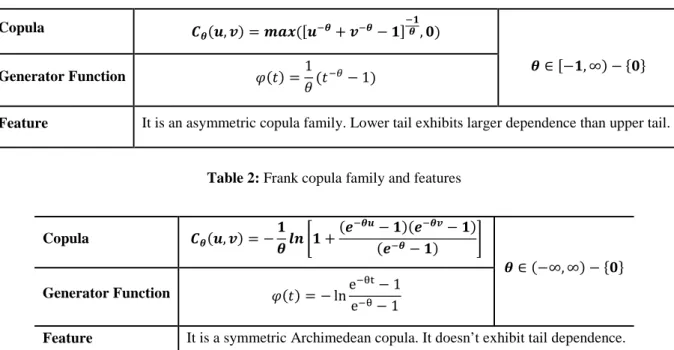
Table 1: Clayton copula family and features

Copula _𝑪𝑪 𝜽𝜽(𝒖𝒖, 𝒗𝒗) = 𝒎𝒎𝒎𝒎𝒎𝒎 ([𝒖𝒖−𝜽𝜽+ 𝒗𝒗−𝜽𝜽− 𝟏𝟏] −𝟏𝟏 𝜽𝜽_{, 𝟎𝟎)} 𝜽𝜽 ∈ [−𝟏𝟏, ∞) − {𝟎𝟎} Generator Function 𝜑𝜑(𝑡𝑡) =1 𝜃𝜃 (𝑡𝑡−𝜃𝜃− 1)

Feature It is an asymmetric copula family. Lower tail exhibits larger dependence than upper tail.

Table 2: Frank copula family and features

Copula 𝑪𝑪_𝜽𝜽(𝒖𝒖, 𝒗𝒗) = −𝟏𝟏 𝜽𝜽 𝒍𝒍𝒍𝒍 �𝟏𝟏 + (𝒆𝒆−𝜽𝜽𝒖𝒖_{− 𝟏𝟏)(𝒆𝒆}−𝜽𝜽𝒗𝒗_{− 𝟏𝟏)} (𝒆𝒆−𝜽𝜽_{− 𝟏𝟏)} � 𝜽𝜽 ∈ (−∞, ∞) − {𝟎𝟎} Generator Function _{𝜑𝜑(𝑡𝑡) = − ln}e−θt− 1 e−θ_{− 1}

(5)

56

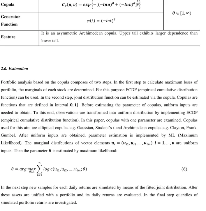
Table 3: Gumbel copula family and features

Copula 𝑪𝑪_𝜽𝜽(𝒖𝒖, 𝒗𝒗) = 𝒆𝒆𝒎𝒎𝒆𝒆 �−[(−𝒍𝒍𝒍𝒍𝒖𝒖)𝜽𝜽+ (−𝒍𝒍𝒍𝒍𝒗𝒗)𝜽𝜽]𝟏𝟏𝜽𝜽�

𝜽𝜽 ∈ [𝟏𝟏, ∞)

Generator

Function 𝜑𝜑(𝑡𝑡) = (−𝑙𝑙𝑛𝑛𝑡𝑡) 𝜃𝜃

Feature It is an asymmetric Archimedean copula. Upper tail exhibits larger dependence than lower tail.

2.6.Estimation

Portfolio analysis based on the copula composes of two steps. In the first step to calculate maximum loses of portfolio, the marginals of each stock are determined. For this purpose ECDF (empirical cumulative distribution function) can be used. In the second step, joint distribution function can be estimated via the copula. Copulas are functions that are defined in interval[𝟎𝟎, 𝟏𝟏]. Before estimating the parameter of copulas, uniform inputs are needed to obtain. To this end, observations are transformed into uniform distribution by implementing ECDF (empirical cumulative distribution function). In this paper, copulas with one parameter are examined. Copulas used for this aim are elliptical copulas e.g. Gaussian, Student’s t and Archimedean copulas e.g. Clayton, Frank, Gumbel. After uniform inputs are obtained, parameter estimation is implemented by ML (Maximum Likelihood). The marginal distributions of vector elements 𝒖𝒖_𝒊𝒊= (𝒖𝒖_{𝒊𝒊𝟏𝟏}, 𝒖𝒖_{𝒊𝒊𝒊𝒊}, … , 𝒖𝒖_{𝒊𝒊𝒎𝒎}) 𝒊𝒊 = 𝟏𝟏, … , 𝒍𝒍 are uniform inputs. Then the parameter 𝜽𝜽 is estimated by maximum likelihood:

𝜃𝜃 = 𝑎𝑎𝑎𝑎𝑎𝑎 𝑚𝑚𝑎𝑎𝑥𝑥

𝜃𝜃𝜃𝜃𝜃𝜃 � 𝑙𝑙𝑙𝑙𝑎𝑎 𝑐𝑐(𝑢𝑢𝑖𝑖1, 𝑢𝑢𝑖𝑖2, … , 𝑢𝑢𝑖𝑖𝑖𝑖; 𝜃𝜃) (6) 𝑛𝑛

𝑖𝑖=1

In the next step new samples for each daily returns are simulated by means of the fitted joint distribution. After these assets are unified with a portfolio and its daily returns are evaluated. In the final step quantiles of simulated portfolio returns are investigated.

3.The Data and Empirical Results

3.1.The Data Description

The data set is composed of five stocks that increased values in İstanbul stock exchange: Goodyear tire & rubber company (GOODY), Doğuş automotive service and trade joint stock company (DOAS), Pegasus airlines

company (PGSUS), TAV airports holding (TAVHL), Turkish airlines corporation (THYAO). The sample begins in 06/05/2014 to 11/10/2016 giving us 611 observations. Asset portfolio is created from this five stock

obtained from İstanbul stock exchange. In this paper, Value-at-risk (VaR) of the portfolio including five stocks: GOODY, DOAS, PGSUS, TAVHL and THYAO are examined via the copula approach. Value-at-Risk (VaR) is a computation used in financial risk evaluation. The goal of this computation is to present some numerical

(6)

57

perception to the risk level of an asset portfolio. This computation gives the maximum potential losses at a certain confidence level. The target of this study is to estimate the one-day later maximum potential losses for the portfolio of stocks constructed with the copula approach. In this sense one of approaches used for the estimation is to assume that the joint distribution of asset returns does not vary during time. In this case results are so close to truth if and only if a small time interval is utilized. Stocks interested in this study have increased in recent times. So, the main result expected is how many maximum loses of investors can be when they buy these stocks for the portfolio.

Table 4: Descriptive statistics of the return series

Goody Doas Pgsus Tavhl Thyao

Mean 0,000796 0,00031 -0,001446 -0,000333 -0,000376 SD 0,023914 0,02109 0,016776 0,016975 0,016826 Skewness 1,336 -1,0833 -0,3403 -0,6057 -0,7531 Kurtosis 16,1955 7,8681 6,5055 8,2171 10,4639 Min -0,1204 -0,1124 -0,0939 -0,1186 -0,1237 5% -0,032 -0,0316 -0,0284 -0,0269 -0,0274 25% -0,0107 -0,009 -0,01 -0,0092 -0,0096 Median 0 0,0012854 -0,0009804 0 0,0008754 75% 0,009 0,0119 0,0085 0,0089 0,009 95% 0,0345 0,0302 0,0249 0,0259 0,0233 Observations 610 610 610 610 610

Table 4 gives descriptive statistics of the series. Non-normality of the data series is clear from the values for skewness and kurtosis.

In this case, the copula approach provides an efficient method to model the dependency among variables. Thus, joint distribution function obtained by means of copulas gives more robust results concerning the portfolio. Gaussian copula model is ignored due to non-normality of the data.

3.2.Empirical Results

In this section, only four copulas are investigated due to nonlinearity of the data. These copulas are Student’s T from elliptical copula, Frank, Clayton and Gumbel from Archimedean copulas. Estimated results for these copulas are demonstrated in Table 5.

The choice of the best fitted copula model is based on Akaike information criterion (AIC) and Schwarz’s Bayesian Criterion (SBC). The results obtained show that the best fitted copulas for the returns of five stocks is Student’s T copula. AIC and SBC values of the copula are -976.4080 and -927.8780, respectively.

(7)

58

Table 5: The estimated results for copulas

Copulas Parameter SE AIC SBC

Student’s T 10,5546 1,9961 -976,408 -927,878

Frank 2,5678 0,1191 -623,8091 -619,3973

Clayton 0,5933 0,0286 -723,7875 -719,3756

Gumbel 1,3402 0,0195 -585,004 -580,5922

The correlation matrix for the best fitted copula is given in Table 6. The results show that correlations between returns of the stocks are rather different. Under all samples there are positive correlations among returns. The strongest correlation is between Pgsus and Thyao. However the correlation between Goody and Doas is the lowest with respect to the best fitted copula. Plots of the returns and transform returns are given in Figure 1. While the returns that have the strongest dependence show denser diffusion along the diagonal, the returns of Doas and Goody that have the lowest dependence exhibit less denser diffusion along it. Dependence path of the best fitted copula are showed in Figure 2. This implies that data simulated from real data represents the same pattern with the returns. In this sense the estimations obtained from the best fitted copula give more robust results. Plots for other copulas are presented in annex (Figure A1. in Annex). After examined the correlation matrix, next step is to simulate data from the best fitted copula to construct the portfolio concerning five stocks. The number of the simulation can be taken the value of 12000.

Table 6: Correlations between returns for the whole sample

Goody Doas Pgsus Tavhl Thyao

Goody 1 0,29963 0,43151 0,3385 0,44601

Doas 0,29963 1 0,44102 0,31492 0,50803

Pgsus 0,43151 0,44102 1 0,43052 0,74103

Tavhl 0,3385 0,31492 0,43052 1 0,46039

Thyao 0,44601 0,50803 0,74103 0,46039 1

Table 7: Descriptive statistics of the created portfolio

Statistics Value Mean -0,00032 SD 0,01625 Variance 0,00026 Median 0,00016 Range 0,30149 Skewness -1,85993 Kurtosis 21,0503 MSE 0,00014

(8)

59

Descriptive statistics of the portfolio created is presented in Table 7. The value of MSE is quite small. This implies that the model selected is appropriate for the portfolio that will be created. The inference from this model is rather robust for calculating the risk regarding the portfolio. In this step of the paper the equally weighted next day portfolio return is evaluated. Firstly each of the returns is transformed into nominal scale. After all returns are given equal weights, the result is transformed into a net return by subtracting one. Eventually empirical quantiles of simulated daily portfolio return are evaluated.

Table 8: The return quantiles of the created portfolio

Quantile Estimate 100 % Max 0,102695 99% 0,040545 95% 0,02153 90% 0,015967 75 % Q3 0,000785

Table 8 shows that the with 99 % maximum potential losses based on an equally weighted portfolio for the next day does not surpass 4 %. In other words, with % 99 maximum potential losses for the portfolio constructed based on the copula approach are 4 %. Maximum potential losses of the portfolio with 95 % and 90 % are 2.1 and 1.5, respectively. For Frank, Clayton and Gumbel copula, the return quantiles of the created portfolio are given in annex (Tables A1-A3).

Figure 1: Dependence path of the returns and the transformed returns, respectively.

(9)

60

4.Conclusion

This study investigated the modelling of dependency. It is quite difficult to determine dependence structure when relationship is nonlinear and distribution of variables is not appropriate for normal distribution. In this case copulas are commonly used and play crucial role in modelling the dependence structure between variables regardless of marginals. In this paper portfolio analysis was performed by considering dependence structure between variables. Five stocks that have increased in value recently were investigated and the portfolio concerning these stocks was constructed. Marginals of each stock were transformed into joint distribution function by taking into consideration dependence structure between variables. The portfolio of these stocks was constructed by means of new joint distribution function obtained. In this analysis each stock was given an equal weight to create the portfolio. Next-day maximum possible losses of the portfolio were computed using the best fitted copula. In consequence of the study it was seen that the copula approach provides crucial flexibilities to construct the joint distribution function. In general the values of stocks are distributed as heavy-tailed. In this case a tool that can be model the best for the stocks is needed. İrrespective of marginals, copulas constructs the joint distribution to evaluate Value-at-Risk. Besides, the copula does not require too much assumption compared to other methods modelling the dependence structure. Since the dependency was modelled correctly, the results obtained using the copulas are rather robust and reliable. On the whole, buying the portfolio of stocks considered will be benefit for investors since the portfolio indicates low risk. In this sense this paper leads the investor to evaluate risk level for the portfolio. Moreover the study guides to investigations in economics field such as banking, insurance in evaluating risk and determining investment tools.

References

[1] Sklar A. “Fonctions de Répartion à n Dimensions et Leur Marges”. Publications de l’Institu de Statistique de l’Université de Paris, 8: 229-231, 1959.

[2] Dimitrova D.S., Kaishev V.K., Panev S.I. “GeD spline estimation of multivariate Archimedean copulas”. Computational Statistics & Data Analysis, 52.7: 3570-3582, 2008.

[3] Genest C., Neŝlehová J., Ben Gharbal N. “Estimators based on Kendall’s tau in multivariate copula models”. Australian & New Zealand Journal of Statistics, 53.2: 157-177, 2011.

[4] McNeil A., Neŝlehová J. “Multivariate Archimedean Copulas, d-Monotone Functions and l_i-Norm Symmetric Distributions”. The Annals of Statistics, 3059-3097, 2009.

[5] Taylor M.D. “Multivariate measures of concordance for copulas and their marginals”. arXiv,1004.5023, 2010.

[6] Berger T., Jammazi R. “On the dependence structure between US stocks: A time varying wavelet-copula-evt approach”, 2015.

(10)

61

Computer Science, 55:1318-1324, 2015.

[8] Righi M.B., Ceretta P.S. “Forecasting Value at Risk and expected shortfall based on serial pair-copula constructions”. Expert Systems with Applications, 42.17:6380-6390, 2015.

[9] de Mello Junior H. D., Marti L., da Cruz A.V.A., Vellesco M.M.R. “Evolutionary algorithms and elliptical copulas applied to continuous optimization problems”. Informaiton Sciences, 369:419-440, 2016.

[10] Joe H. Multivariate models and dependence concepts. London and New York: Chapman & Hall/CRC monographs on statistics & applied probability, 1997.

[11] Roger B.N. An Introduction to Copulas. New York: Springer series in statistics, 2006.

Appendix

Table A1: The return quantiles of the created portfolio with respect to Frank copula

Table A2: The return quantiles of the created portfolio with respect to Clayton copula

(11)

62

Table A3: The return quantiles of the created portfolio with respect to Gumbel copula