FREQUENCY DOMAIN FATIGUE
ANALYSIS OF DYNAMICALLY
SENSITIVE STRUCTURES
Ruhuai Wang
A Dissertation subm itted for the Degree of
Doctor of Philosophy
Departm ent of Mechanical Engineering
University College London
ProQ uest Number: 10017445
All rights reserved
INFORMATION TO ALL U SE R S
The quality of this reproduction is d ep en d en t upon the quality of the copy subm itted.
In the unlikely even t that the author did not sen d a com plete manuscript
and there are m issing p a g e s, th e se will be noted. Also, if material had to be rem oved, a note will indicate the deletion.
uest.
ProQ uest 10017445
Published by ProQ uest LLC(2016). Copyright of the Dissertation is held by the Author.
All rights reserved.
This work is protected against unauthorized copying under Title 17, United S ta tes C ode. Microform Edition © ProQ uest LLC.
ProQ uest LLC
789 East E isenhow er Parkway P.O. Box 1346
A b stract
Contents
A b stra ct i
Table o f C on ten ts i
L ist o f Figures v
L ist o f Tables viii
N o m en cla tu re ix
A ck n ow led gem en ts x v
D eclaration x v i
1 IN T R O D U C T IO N 1
1.1 In tro d u c tio n ... 1
1.2 Outline of the T h e s i s ... 8
1.3 New D e v e lo p m en ts... 8
1.3.1 A new frequency domain theoretical a p p r o a c h ... 8
1.3.2 Effect of non-G aussianality... 12
1.4 A p p licatio n s... 13
1.5 Arrangement of the T h e s is ... 14
2 T H E O R E T IC A L B A C K G R O U N D 16 2.1 Fatigue Failure and Palmgren-Miner Cumulative Damage Hypothesis (Linear Damage R u l e ) ... 16
2.2 Random Process ...20
2.2.1 Basic c o n c e p t ...20
2.2.2 Moments and characteristics fu n c tio n ...21
2.2.3 Correlation (covariance) f u n c t i o n ...23
2.2.4 Power spectral density ( P S D ) ... 23
2.2.5 Fast Fourier transform ( F F T ) ...24
2.2.6 Statistics in the frequency d o m a in ... 26
2.3 Response Spectrum of Dynamic S y ste m ... 29
2.4 Level Crossing and Distribution of E x t r e m a ... 31
2.4.1 Level c ro s s in g ...32
C O N TE N TS ii
2.4.3 Distribution of e x tre m a ...37
2.5 Stress (Strain) cycle c o u n t i n g ... 37
2.6 Rainflow Cycle C o u n tin g ... 39
2.6.1 Original definition ... 39
2.6.2 Alternative d e f in itio n s ...39
3 E X IS T IN G F R E Q U E N C Y D O M A IN M E T H O D S 45 3.1 Analytical Solutions ... 45
3.1.1 Steinberg’s three-band t e c h n i q u e ... 45
3.1.2 Narrow band so lu tio n ...46
3.1.3 Wide band s o lu tio n ... 48
3.1.4 Tunna’s fo rm u la ... 50
3.2 Correction Factor Solutions— Empirical F o rm u la e ... 51
3.2.1 Wirsching’s formula ...52
3.2.2 Kam, Chaudhury and D o v e r... 52
3.2.3 H a n c o c k ... 52
3.2.4 Madsen ... 53
3.2.5 O r t i z / C h e n ... 56
3.2.6 L a r s e n /L u te s ...56
3.2.7 Dirlik ...57
3.3 Bishop’s Theoretical A p p r o a c h ... 58
3.4 D iscu ssio n ... 59
4 A P P L IC A T IO N S TO W E G A N D H O W D E N W IN D T U R B IN E DATA 61 4.1 In tro d u c tio n ...61
4.2 The WEG and Howden Wind Turbine D a t a ...62
4.2.1 WEG MS-1 d a t a ... 62
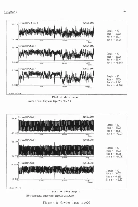
4.2.2 Howden HWP 330 data ...63
4.3 Analysis P r o g ra m ... 64
4.4 Statistical A n a ly s is ... 68
4.4.1 Pre-processing of the measured data ... 72
4.4.2 Basic statistics ...73
4.4.3 Stationarity and trend t e s t s ... 73
4.4.4 Testing for normality (G a u ssia n a lity )... 74
4.4.5 R e su lts... 76
4.5 PSDs of WEG and Howden D a t a ... 78
4.6 Fatigue Life Prediction Results ... 82
4.7 Practical Considerations in the Calculation ...85
4.7.1 Choice of cutoff f re q u e n c y ...94
4.7.2 Effect of S-N curve s lo p e ...96
4.7.3 Effects of b a n d w id th ... 102
C O N T E N T S iii
5 E F F E C T OF D E T E R M IN IS T IC C O M P O N E N T 115
5.1 In tro d u c tio n ...115
5.2 Separation of a Deterministic Component From Mixed S ig n al... 117
5.2.1 Band pass f i l t e r ... 117
5.2.2 Least square sine wave f i t t i n g ...117
5.3 The Program for Carrying Out the S tu d y ...118
5.4 M ixture of Stationary Signals with Sine W a v es... 119
5.5 M ixture of Stationary Signals with Equally-spaced S p ik e s...124
5.6 C onclusion... 128
6 A N E W T H E O R E T IC A L A P P R O A C H 132 6.1 In tro d u c tio n ...132
6.2 A New A p p r o a c h ... 132
6.2.1 Definitions ... 132
6.2.2 Peak-peak transition p ro b a b ility ... 134
6.2.3 Peak-peak transition with lowest trough to the r ig h t ... 137
6.2.4 Peak-peak transition with lowest trough to the l e f t ... 138
6.2.5 Rainflow transition p ro bability ...139
6.2.6 The probability density function of rainflow cycle ranges . . .1 4 0 6.3 Flow chart of c a lc u la tio n ... 140
6.4 Kowalewski’s Joint p.d.f. of Adjacent Peaks Sz T r o u g h s ... 141
6.5 Peak Value Probability Density F u n c tio n ... 145
6.6 Examples of the A p p lic a tio n s ... 147
7 L IN K B E T W E E N N O N -G A U S S IA N A L IT Y A N D FA T IG U E LIFE 155 7.1 In tro d u c tio n ...155
7.2 M athematical Description of Non-Gaussian Random Processes . . . . 156
7.2.1 Basic concepts... 156
7.2.2 M athematical description of non-gaussian random variables . . 158
7.3 Statistical Description of Non-Gaussian Process: Time Domain and Frequency D o m a i n ... 161
7.3.1 Time d o m a i n ... 162
7.3.2 Frequency domain ... 163
7.4 Methods Dealing W ith Non-Gaussianality in Random Fatigue Analysis 163 7.4.1 Gorrection factor a p p ro a c h ... 164
7.4.2 Koliopulos’s “separability” a p p r o a c h ... 166
7.5 Peak-trough Series R egeneration... 166
7.5.1 Transition m a t r i x ...166
7.5.2 Load sequence generation ... 167
7.6 Modelling the Effect of N o n -G a u ssia n a lity ... 168
7.6.1 Outline of the m o d e llin g ...170
7.6.2 Simulation of stationary Gaussian process... ... 171
7.6.3 Regeneration of Non-Gaussian s i g n a l ... 173
C O N TE N TS iv
8 M O D E L L IN G T H E E F F E C T OF N O N -G A U S S IA N A L IT Y 183
8.1 Procedure of S im u la tio n ...183
8.2 Artificial Neural Network (ANN) (Backpropagation) ... 189
8.2.1 The c o n c e p t... 189
8.2.2 Neural n etw o rk s... 190
8.2.3 The processing elements of a neural n e tw o r k ... 192
8.2.4 Transfer functions and local memories ...193
8.2.5 Training of a neural network and learning la w s ... 194
8.2.6 Artificial neural networks (b ac k p ro p ag a tio n )... 195
8.3 ANN to Model Rainflow Range p.d.f. for Non-Gaussian Signals . . . 198
8.3.1 Program and flow chart ...198
8.3.2 Choice of neural network structure and p a r a m e t e r s ...198
8.3.3 R e s u lts... 199
8.3.4 Application of the toolbox to WEG and Howden d a t a ...199
8.4 Summary and C o n clu sio n s... 200
9 C O N C L U S IO N S A N D F U R T H E R W O R K 207 9.1 Summary and C o n clu sio n s... 207
9.2 Recommended Future W o r k ...210
R eferen ces 212
A S P E C T R A L FA T IG U E A N A L Y SIS P R O G R A M 222
List of Figures
1.1 Outline of the thesis ... 9
1.2 A new theoretical approach ... 10
1.3 Study of the effect of non-Gaussianality ... 11
2.1 Generalised S-N c u r v e ... 17
2.2 PSD moments c a lc u la tio n ...27
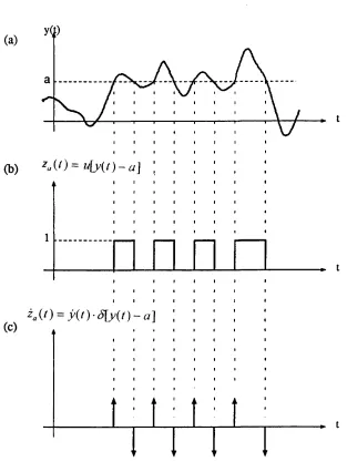
2.3 A sample function of y[t) and the defined associated processes . . . . 33
2.4 Example of RFC-counting m e th o d ...40
2.5 Rychlik’s new definition of RFC counting ... 41
2.G Modified definition for rainflow c y c l e ... 41
2.7 Bishop’s definition for rainflow cycle ... 43
2.8 An example of rainflow cycle counting ...44
3.1 Generalised S-N curve ... 48
4.1 WEG MS-1 wind turbine blade data: y 12c, yl9f, y27a, y 3 5 d ... 65
4.2 Howden data: tape2G ...GG 4.3 Howden data: Edgewise: tape2G-chG,8,10, Z o o m e d ... G7 4.4 Example of first set of simulated data: n h d a t c...G9 4.5 Rainflow Cycle Range PD F of n b d a t a... 72
4.G Amplitude distribution of WEG Y 12a d a t a ... 77
4.7 Amplitude distribution of Howden H2G05 Flapwise d a t a ... 77
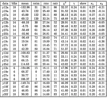
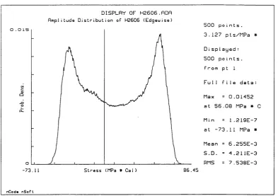
4.8 Amplitude distribution of Howden H2G0G Edgewise d a t a ...79
4.9 PSD of WEG data: y27a - linear s c a l e ... 79
4.10 PSD of WEG data: y27a - logarithm scale ... 80
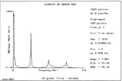
4.11 PSD of Howden data: Tape2G-cli5...80
4.12 PSD of HWP26 (logarithm scale): Tape26-chG ...81
4.13 Cycle range probability density functions for W EG MS-1 d ata yl2a,b,c,f 84 4.14 Rainflow cycle range probability density functions for Howden flap- wise data Tape 27, channel 5...86
4.15 Rainflow cycle range probability density functions for Howden edge wise data. Tape 27, channel 6...87
4.16 Influence of cutoff frequency of WEG MS-1 d a ta y 12a ...97
4.17 Influence of cutoff frequency of Howden data, tape 26- 5m flapwise . 98 4.18 Influence of cutoff frequency of Howden data, tape 26- 5m edgewise . 99 4.19 Effect of S-N curve slope : WEG MS-1 data v 3 5 d ... 100
L IS T OF FIGURES vi
4.21 Effect of S-N curve slope: Howden data tape 27 3m f la p w is e ... 103
4.22 Effect of S-N curve slope: Howden data tape 27 3m ed g ew ise... 104
4.23 Effect of the S-N curve slope: Wirsching S o l u t i o n ...105
4.24 Effect of the S-N curve slope: Steinberg S o lu tio n ... 106
4.25 Effect of the Bandwidth: Narrow Band S o lu tio n ... 107
4.26 Effect of the Bandwidth: Wirsching S o lu tio n ... 108
4.27 Effect of the Bandwidth: Steinberg S o l u t i o n ... 109
4.28 Effect of the Bandwidth for Fatigue life: Dirlik S o lu tio n ... 110
4.29 Clipping of normal d i s t r i b u t i o n ... 112
4.30 Choice of clipping ratio: WEG data y 2 7 d ...113
4.31 Choice of clipping ratio: Howden data tape 26 3m fla p w is e .113 4.32 Choice of clipping ratio: Howden data tape 26 3m edgew ise.114 5.1 XFILE, the sine wave and the mixed signal ... 120
5.2 An example of PSDs of XFILE, the sine wave and the mixed signal . 121 5.3 Histogram of rainflow cycle range-mean distribution of XFILE . . . . 122
5.4 Histogram of rainflow cycle range-mean distribution of a mixed file . 123 5.5 Effect of mixing sine wave with XFILE, S-N slope b = 4 ...125
5.6 Effect of mixing sine wave with XFILE, S-N slope b = 7 ...126
5.7 Effect of mixing sine wave with XFILE, S-N slope b=10 127 5.8 Effect of mixing spikes with XFILE, S-N slope b = 4 ... 129
5.9 Effect of mixing spikes with XFILE, S-N slope b = 7 ... 130
5.10 Effect of mixing spikes with XFILE, S-N slope b=10 131 6.1 Discretization of the signal ...133
6.2 transition probability ... 134
6.3 M atrix 136 6.4 flow chart of the c a lc u la tio n ...142
6.5 Joint p.d.f. of adjacent peaks and troughs of a Gaussian Signal . . . 146
6.6 Peak Value p.d.f. of a Gaussian Signal: G am m a= 0.01, 0.255, 0.5, 0.745, 0.99 148 6.7 Cycle Range PDF for WEG data: y l 2a & b ... 149
6.8 Cycle Range PDF for WEG data: y27a & b ... 150
6.9 Cycle Range PDF for WEG data: y27c & d ... 151
6.10 Cycle Range PD F for WEG data: y27e & f ... 152
6.11 Cycle Range PD F for Howden data: H26: 5m Flapwise & Edgewise . 153 7.1 procedure for regenerating a loading sequence from a transition m atrix 168 7.2 P D F ’s from regenerated load sequence: WEG y 3 5 d ...169
7.3 Flow chart of digital generation of Non-Gaussian Stochastic Signal . 176 7.4 The relationship of param eter and k u r to s is ...177
7.5 Nonlinear transform ...178
7.6 Simulated non-Gaussian Signal: example 1 179
7.7 Simulated non-Gaussian Signal: example 2 180
7.8 Simulated non-Gaussian Signal: example 3 181
L IS T OF FIGURES vii
8.1 Power Spectral Density s h a p e s ... 185
8.2 An example of the Rainflow Range p.d.f with different kurtosis . . . . 188
8.3 A typical neural network a rc h ite c tu re ...192
8.4 An illustration of a processing e l e m e n t ... 193
8.5 Layout of back propagation n etw o rk ...195
8.6 Flow chart of backpropagation p ro g ra m m in g ... 201
8.7 A typical error s u r f a c e ... 202
8.8 Comparison of PDFs by trained neural network: example 1: sp7, kurtosis= l & 4 ...203
8.9 Comparison of PDFs by trained neural network: example 2: sp27, kurtosis=0.5 & 3 ... 204
8.10 Example of PDFs predicted by the toolbox: WEG data ... 205
8.11 Example of PDFs predicted by the toolbox: HOWDEN d a t a ...206
List of Tables
4.1 WEG MS-1 Wind Turbine Blade load cases ... 63
4.2 Howden HWP330 data load c a s e s ...63
4.3 Comparison of Fatigue damage prediction by different methods: Sim ulated data: Part 1 70 4.4 Comparison of Fatigue damage prediction by different methods: Sim ulated data: Part 2 71 4.5 95% Confidence Region of Reverse Arrangement T e s t ... 74
4.6 Results of Statistical Tests on W FC D a t a ...78
4.7 Statistics of Howden HWP 330 d a t a ...82
4.8 Comparison of Fatigue Life results using the different methods: W FC data, Part 1 ...85
4.9 Comparison of Fatigue Life results using the different methods: W FC data, Part 2 ...88
4.10 Comparison of Fatigue Life results using the different methods: W FC data. Part 3 ...89
4.11 Comparison of Fatigue Life results using the different methods: W FC data. Part 4 ...90
4.12 Comparison of Fatigue Life results using the different methods: How den data. Part 1 (ch5, ch7 and ch9 are flapwise, ch6, ch8 and chlO are e d g e w is e ) ... 91
4.13 Comparison of Fatigue Life results using the different methods: How den data. Part 2 (ch5, ch7 and ch9 are flapwise, ch6, ch8 and chlO are e d g e w is e ) ... 92
4.14 Comparison of Fatigue Life results using the different methods: How den data. Part 3 (ch5, ch7 and ch9 are flapwise, ch6, ch8 and chlO are e d g e w is e ) ... 93
6.1 Fatigue Damage rates calculated by the new m e t h o d ... 154
8.1 70 PSD’s used in stress history simulation (1) ...186
8.2 70 PSD ’s used in stress history simulation ( 2 ) ... 187
NOMENCLATURE
General
PSD Power Spectral Density
PD F, p.d.f., pdf Probability Density Function D FT Discrete Fourier Transform F F T Fast Fourier Transform
RAT Reverse Arrangement Test
FEA Finite Element Analysis ANN Artificial Neural Networks
RMS, rms root mean square
S stress cycle range
5*0, Sc transition stresses
N cycle number
b, hi, 62 inverse slopes of S-N curve
c, Cl, 02 A curve intercepts
V for all
Chapter 2
A D damage ratio
D accumulated fatigue damage
E[P] expected peak number in unit tim e (peak frequency) J5[0] expected zero-crossing number in unit tim e
p{S) probability density function of cycle ranges
Sh Equivalent Stress Param eter
uj radius frequency
S{lü) double-side (radius frequency) PSD
G{f) single-side Hertz PSD
nin (n= 0,l,2...) n-th moment of the one-sided Hertz PSD
Mn (n= 0,l,2...) n-th moment of the double-sided radius PSD
a crack size
ao initial crack size
C, m crack growth constants
A K stress intensity factor range
F (a) a geometry function
X { t ) , y{t), Za{t) random processes
Nomenclature
t tim e
T tim e lag
T tim e duration
P(x) probability distribution of x p(x) probability density function of x
CX-n Tith order moment
(J'n nth order central moment
X mean value of random process
(T root mean square
E{.] m athem atical expectation
characteristic function
Rxy cross-correlation function
Rx autocorrelation function
Rxx autocorrelation function
^ni Fourier constants
X(w) Fourier integral
A{iü) real part of X(w)
B(w) imaginary part of X(w)
% stochastic process
X first order differential process X second order differential process
power spectral density function
Ls duration of signal
A t tim e interval width of signal
7 irregularity factor
fmi mean frequency
M mass m atrix
C damping m atrix
K stiffness m atrix
V deformation
p{r) loading
Tp period of load
K ' ) unit impulse response function
Fourier transform of load p(t)
tim e domain response
y(2w) frequency domain response
^ (w ) frequency response function
5'(2W) response spectrum
w[-] unit step function
Dirac delta function
sign{-) sign function
number of level (a) crossing in unit time number of down level (a) crossing in unit tim e number of upper level (a) crossing in unit tim e
Nomenclature xi
Chapter 3
(j = y/m^ root mean square
E[D] expected damage
b,c m aterial (S-N curve) parameters
Sh equivalent stress param eter
7 irregularity factor
E[P] expected peak number in unit time (peak frequency) E [0] expected zero-crossing number in unit tim e
r ( ') Gamma function
E[D]n b expected damage by narrow band solution
Q{x^\i') chi-square probability function
p correction factor for the fatigue damage rate
erf{') error function
z normalised cycle range (= S /2y/mô )
Pr r{z) rainflow cycle range PDF Cl coefficients in Dirlik’s formula
C2 coefficients in Dirlik’s formula
C3 coefficients in Dirlik’s formula r factor of exponential distribution
a factor of Rayleigh distribution
Yi first event in rainflow cycle
Y2 second event in rainflow cycle I 3 third event in rainflow cycle l i ( ) probabilities of Yi
probabilities of Y2 I 3O probabilities of I 3
ip peak level
kp trough level
dh level interval width
Chapter 4
N number of signal blocks
RAT reverse arrangement test
p mean value
(7^ variance
S.D. standard deviation
R M S root mean square
a significant level
A number of reverse arrangements
chi-square distribution
Nomenclature xii
Cal calibrated factor
p clipping ratio
Xmax assumed maximum value of random process
Chapter 5
X(t) stochastic response caused by the wind turbulence
Y(t) gravity induced response
Z(t) combined response
A am plitude of the harmonic component
D global mean value of the signal
(j) = Lût azimuth
( a suitable initial phase
cTx = \/TÜô Root Mean Square
= mean frequency
•' mo Y ^4
A amplitude
/ frequency
Chapter 6
y[t) loading history
{y{i):i = 1,2, ...N] sequence of extrem a
M number of levels
si, S2, ...s m values of levels
A interval
p(-) probability density function
Pk{vj) probability of peak (trough) falling in interval k (j)
Pkiÿj) probability of peak (trough) falling above (below) interval k (j)
tjk,Ujk,djk transition probabilities
T , U , D transition probability matrices
m , k , i , j , l indices for extrem a
probability of a transition from a peak Sk to another peak Si with n troughs inbet ween
Ij, Gki Hk special matrices
rightwards PDF
ll. leftwards PDF
PR{k) rainflow cycle range PD F with range k X
E[P] = expected value of the number of peaks per unit tim e (peak frequency)
E[PI] = expected value of the number of inflection points per unit tim e (inflection point frequency)
Nomenclature X l l l No Ni Cl,C2 1 OL-m OLa ai «2 J sign{‘) a = y/mo
and mean values of adjacent extremes zero crossing frequency
peak frequency parameters
irregularity factor mean value amplitude trough value peak value Jacobi an sign function
normalised peak value error function
x (t) P(x)
Xo
R
71 = ^
72 = ^ - 3
Xu — 1-5 2, ...)
Ck (k=3,...n)
Hk{x) (k=3,...n)
^mn
& 6 6, c h ^mn ^mn ^ 4 0 5 ^ 0 4 r (0
Xk (k=3,...n)
Hp G[.]
w
Rxxilll ^
2)
Rxxxi^l 1 l'2'i
^
3)
R x x x x i l ' l5^ 2 5 ^ 8 5^
4)
E[]
^1,
t2,
to,^4T,Ti,T2,T3
Chapter 7 random process
joint probability density function (p.d.f.) mean value vector
Covariance Matrix skewness
kurtosis
distribution function characteristic function cumulants (semi-invariants)
Gaussian probability density function constants
Hermite polynomials unit function
stress process and its derivative m aterial constants
cumulants
“normalized” cumulants kurtosises of ( and Gamma function cumulants
entropy
nonlinear function a param eter
autocorrelation function
3rd order correlation (Bi-correlation) 4th order correlation (Tri-correlation) ensemble average
Nomenclature XIV
S x x x i ^ ^ l 5^ 2) S x x x x( ^ 1 5^ 2 5^ 3 )
g ( ' )
X, mo;
(n—0,1,...)
VD
« 1, 0:2
P m a x , m i n ( ^ ^ l ^0
:
2)
7 mo
bi-spectrum tri-spectrum
standard normal process monotonie transfer function mean value of x
parameters
mean damage accumulation rate trough, peak value
joint PDF of adjacent peaks and troughs irregularity factor
0-th moment of PSD (variance)
Chapter 8
a 1 Xjn
s
G{ f )Ai, fi ,Q i (i= l,2 )
fc net.' P 3
Wiij
' p i
^pk
&
%
root mean square irregularity factor mean frequency cycle range
single-side Hertz PSD parameters
cutoff frequency input to neuron j
from system input p
weight factor of neuron
i to neuron j
output of neuron i for system input p
error at neuron k
for system input p
total error of output layer coefhcient of sigmoid function interm ediate quantity
A ck n ow led gem en ts
I would like to express thanks to my supervisor, Dr. Neil Bishop, for his guidance, help and encouragement during the course of my research.
I am also indebted to Stuward Kerr and Andrew Halfpenny who have read and commented on part of the dissertation.
I would like to thank my parents, my wife Zhinong and my daughter Cherry for their love and support. W ithout their support, this thesis could never have been finished.
Ruhuai Wang
D ecla ra tio n
This dissertation is subm itted in support of an application for the Degree of Doctor of Philosophy in Engineering Science, from University College London, University of London.
No part of the work contained in the thesis has been subm itted for any other Degree or Diploma from this University or any other Institution.
All the computation work in this thesis was performed by programs coded and developed by me unless otherwise stated in the text.
I hereby declare th at this declaration is true in every respect.
Ruhuai Wang
Chapter 1
INTRODUCTION
1.1
I n tr o d u c tio n
The aim of using stochastic process theory for structural analysis is to judge the reliability of a structure which has been designed to w ithstand random loading. The most common structural failures are first-excursion failures and fatigue failures, particularly the latter which account for the majority of all service failures due to mechanical causes (in metallic structures, it has been claimed th at some 80-90% of failures are related to fatigue and fracture[22]). Traditionally, fatigue damage prediction is carried out in the tim e domain, th at is, using tim e histories of response (stress or strain) to estim ate fatigue life. In recent years, several frequency domain techniques[14, 17, 18, 19, 94, 93] have been developed to predict fatigue life. Rather than directly using the measured stress signal, these methods predict fatigue life from the Power Spectral Density (PSD), or the relevant moments, of the stress signal. In many engineering fields this is sometimes the only loading information which is available, particularly at the design stage. Also, in some engineering applications, e.g., the aircraft industry, standard loading spectra (PSD, etc.) have been developed, which precisely simulate the service environment. The frequency domain approaches (spectral fatigue methods) can then be applied to produce more reliable designs.
Fatigue is defined as the process of progressive localized permanent structural change occurring in a material subjected to conditions which produce fluctuating
stresses and strains at some point or points and which may culminate in cracks or
complete fracture after a sufficient number of fluctuations [7] [12]. Fatigue of metals
chapter 1 2
has been studied for over 150 years [34, 8, 35]. The first fatigue investigation seem to have been reported by a German mining engineer, W.A.S. Albert, who in 1829 performed some repeated loading tests on iron chain[26]. During the period from 1852 to 1870, a German railway engineer, August Wohler, set up and conducted the first system atic fatigue investigation. These experiments were conducted to establish a safe alternating stress below which failure would not occur. Full scale axles as well as smaller laboratory specimens were employed to establish the endurance limit concept for design. Many im portant aspects of fatigue behaviour were pointed out. The most im portant one being th at fatigue depends more on the range of stress than the maximum stress and the life of specimens reduces when the amplitudes of repeated loading increases. Test data were plotted on what has become known as the S- N diagram, and fatigue data today are often presented in much the same way.
After the initial research from 1850 to 1875, more experimental work was con ducted to establish a clearer understanding of the fatigue phenomena[8], i.e., the process of crack propagation under cyclic loading. The importance of cyclic defor m ation was clearly established in 1930’s. Research in fatigue during the 1930’s and 1940’s was largely devoted to experimentally establishing the effects of the many factors th at influence the long-life fatigue strength. Tests were usually conducted in rotating bending and the life range of interest was about 10® cycles and greater.
During the 1950’s the quantitative relationships between plastic strain and fa tigue life was established. Many significant contributions were made during the 1960’s. Fracture mechanics was developed as a practical engineering tool for fatigue analysis. Paris[76] quantified the relationships for fatigue crack propagation. By the 1970’s fatigue analysis became an established engineering tool in many industrial applications.
There are three m ajor approaches to analysing and designing against fatigue failures [31] [86]. They include:
chapter 1 3
in the component is used to predict its life. The stress is often a nominal stress and local features such as holes and notches are dealt with by introducing stress concentration factors. Failure may be taken as the appearance of a crack, a specific length of crack, or total failure depending on the test data available.
(ii) T h e fracture m echanics approach [83]. Crack propagation is assumed to depend on a fracture mechanics param eter, usually the range of crack tip stress intensity factor A K . Life is then calculated by assuming an initial crack length and finding how many cycles are needed to make this crack grow to an unacceptable size.
(iii) T h e local stress-strain or critical lo ca tio n approach [84] [103]. The strain history of some critical location is estim ated from the nominal loading history, including plasticity effects. Life is then estim ated from test data taken under strain controlled conditions.
The nominal stress approach is used in this thesis. It is chosen because methods such as the other ones described above, either have no relevant influence on the focus of the present study, or are unsuitable for dealing with the loading problem investigated because there is a need to define a stress (or strain) “cycle” for the loading conditions which are more complex than constant amplitude. The nominal stress approach is best suited to so-called long life (low stress) situations where plasticity effects are small. Fortunately for dynamic or vibration problems, where frequency based fatigue tools are particularly relevant, this is usually the case.
chapter 1 4
from the loading tim e history. For the first problem, Miner’s rule[71] is generally adopted. This rule assumes a linear fatigue accumulation and ignores the order of cycles of different range and their interactive effects [82]. For the second problem, many methods of defining or counting a “cycle” have been proposed. Among them , the rainflow cycle counting method [72] is generally used because it is believed th at this m ethod gives the best correlation with test results. The original definition of Rainflow Cycle Counting is complicated, Rychlik[79] gave an alternative definition and proved it is equivalent to the original one. The new definition enables easier application.
In general, stochastic loading is hard to express using a conventional m athem at ical formula. A probabilistic description is usually inevitable. A common way is to express the loading in the frequency domain as a PSD, as with, for instance, wind loading, sea wave loading, etc. In most cases the structure and/or component is assumed to be linear, i.e., the response spectrum can be linearly linked to the loading spectrum by the frequency response function. This analysis technique has many advantages. The most im portant one is th at, the tedious and tim e consuming computing work in the time domain can be avoided and the response spectrum can be obtained without knowing the tim e history of the loading (actually it is very difficult to know). W ith most Finite Element packages used for structural analysis, such spectra can be obtained directly.
It is for this reason that considerable attention has focused on the spectral fatigue analysis approach for structures and/or components subjected to stochastic load ings [12]. This approach uses frequency domain information describing structural response to predict the fatigue damage, rather than relying on the more traditional determ inistic or tim e domain solutions.
calculât-chapter 1 5
ing the number of peaks and zero crossings per unit tim e from the joint probability density function of the process and its first and second order differential processes. For a Gaussian signal, this joint probability density function can be determined from the frequency domain representations of the loading. This relationship provides the basic foundation for spectral fatigue analysis.
The simplest fatigue damage estim ation method is the so-called “Three-Band Technique” [88], which can be regarded as either a tim e domain method or frequency domain method. It can only give a very rough estimation.
chapter 1 6
but the calculation procedure is complicated and susceptible to com putational in stabilities. For this purpose, a new theoretical solution is derived in this thesis and presented in chapter 6. Furthermore, all existing approaches require the stress signal to be stationary, Gaussian and random, i.e. without any significant deter ministic component. Perhaps there are two reasons for this assumption. The first is th a t, according to the central limit theorem^ if there is no significant determ in istic component in the loading, the structural responses should be Gaussian. The second is th at, conventional one-dimensional Power Spectral Density functions can only provide enough information about the distribution of Gaussian processes. Re cent studies[17, 18] show th at the effect of non-Gaussianality cannot be ignored, at least for the Howden HWP330 wind turbine blade data. In some cases the effect is significant. Experience suggests kurtosis is the best and simplest param eter for the description of the departure from the Gaussian distribution. It is known that the distribution of the process and its first and second order differential processes is essential for such analysis. For non-Gaussian responses, there is currently no efficient way to perform the fatigue analysis using frequency domain information. Actually, non-Gaussian processes are too wide a class of distributions to deal with as a whole. In this thesis, efforts are made to study the effect of ^wr^oses-described non- Gaussian signals. This is achieved by applying extensive simulation and artificial neural networks.
chapter 1 7
there is therefore a combined stochastic (wind loading) and determ inistic (gravity) mixed signal. Such a deterministic component makes the response a m ixture of a random process with a strong deterministic component. Effects of mixing a station ary signal with various deterministic components can be found in [19] and chapter 5.
In this thesis, the problems of non-Gaussianality have been studied. For over coming the difficulties of assuming Gaussian, narrow band loading, or applying correction factors, a new frequency domain based approach has been developed[94]. This approach itself doesn’t require the signal to be Gaussian. The PSD of the stress signal is used to predict the probability density function of rainflow cycle ranges (for a non-Gaussian signal, the tri-spectrum is also required). Calculations confirm it is efficient and easy to apply. For Gaussian signals, Kowalewski’s[60] joint PDF of adjacent peaks and troughs is applied. For non-Gaussian signals, an alternative expression for the joint PDF of adjacent peaks and troughs is required. Unfortu nately, due to the m athem atical difficulty of the problem, there is no closed form theoretical expression available. Extensive simulation and modeling was carried out and an Artificial Neural Network (ANN) has been applied to study the effect of non-Gaussianality. A trained network is provided as a toolbox for frequency do main fatigue analysis of general stationary signal (Gaussian or kurtosis-described non-Gaussian).
chapter 1 8
spectral density, tri-spectrum , (in the frequency domain) is required.
1.2
O u tlin e o f th e T h e sis
An outline of the thesis is given in Fig. 1.1. The main achievements are: (i)development of a new theoretical approach (Fig. 1.2) which can be applied to a wide range of ran dom stationary stress loadings; (ii) study of the effect of non-Gaussianality (Fig. 1.3) with Monte-Carlo simulation and artificial neural networks, neural networks are trained to provide a fast, efficient toolbox for practical engineering applications; (iii) a sophisticated study of the factors affecting the accuracy of spectral fatigue analysis; (iv) development of a software package which applies some of the popular frequency domain methods and the new theoretical method. Part of the work has been incorporated into the software product {NSOFT FATIMAS-SPECTRAL) of
nCode International}^.
1 .3
N e w D e v e lo p m e n ts
1.3.1
A n ew freq uency d om ain th e o r e tic a l approach
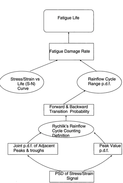
A new frequency domain theoretical approach[94] has been developed to calculate the pdf of rainflow cycle ranges and hence the fatigue life. It is based on Rychlik’s alternative definition[79] of rainflow cycle ranges. The m ethod itself doesn’t require the signal to be Gaussian. For a Gaussian signal, Kowalewski’s joint PD F of ad jacent peaks and troughs can be applied. The forward and backward peak-peak transition (with any number of interm ediate troughs in between) probability m atri ces are calculated. Two cases have been considered. Firstly peak-peak transitions with the lowest trough to the right and secondly with the lowest trough to the left. Rainflow transition probability and therefore the p.d.f. of rainflow cycle ranges has been calculated. Calculations confirm it is efficient and easy to apply. Work has
chapter 1
Joint PDF o f Adjacent Peaks and Troughs
Peak Value PDF
Monte-Carlo Simulations
Non-linear Transform of Gaussian Process
Fatigue Analysis: Frequency Domain Approach
Effect o f non-Gaussianality A New Theoretical
Approach
Artificial Neural Networks (ANN )
Case Studies
Howden HWP 330 Wind Turbine Blades Wind Energy Group
MS-1 Wind Turbine Other Data
chapter 1 10
Flow Chart of the New Method
/
Fatigue Life
V
J
Fatigue D a m a g e R ate
S tress/Strain v s Life (S-N ) Curve
Rainflow C ycle R a n g e p.d.f.
Forward & Backward Transition Probability
Rychlik’s Rainflow C ycle Counting
efinition
Joint p.d.f. of Adjacent P ea k V alue
P ea k s & troughs p.d.f.
P SD of Stress/Strain
chapter 1 11
Effect of Non-Gaussianality
Fatigue Life
S-N Curve
Artificial Neural Networks
Rainflow C ycle R an ge p.d.f.
M onte-Carlo Sim ulation
KurtosisMth Cumulant
Non-linear Transform of G au ssian P r o c e s s
Tim e Domain: S tatistics
Frequency Domain: 1,2,3-D im en sion al P S D
chapter 1 12
been carried out to validate the method for various engineering applications, includ ing WEG (Wind Energy Group) MSI and Howden HWP330 wind turbine blade data.
1.3.2
E ffect o f n on-G au ssian ality
Efforts have been made to get the joint probability density function of adjacent peaks and troughs for general stationary (not necessary Gaussian) signals. Due to m athem atical difficulties, no closed form theoretical results have been achieved. Ex tensive computer modelling[93] (using various methods, including use of the Monte- Garlo method) and Artificial Neural Network (ANN) have been applied to study the effect of non-Gaussianality. For non-Gaussian stress signals, the rainflow cycle range p.d.f. appears to be related to several parameters, these being the root mean square of the signal, the irregularity factor, and kurtosis, a param eter representing the non-Gaussianality of the signal. Analysis of WEG, HWP data and simulation suggests kurtosis as the best description of the degree of the departure from Gaussian distribution. Among various developed Artificial Neural Network systems, back-p roback-p agation , a method of training a neural network to approximate any function, including arbitrarily complex nonlinear functions, is the only neural network tech nique to produce any number of fielded applications. Even though backpropagation has played a key role in the development of artificial neural networks, it is really a statistical modeling technique. More specifically, it is a non-param etric modeling m ethod: one in which the shape of the relationship between inputs and outputs is decided by the data rather than predetermined by the tool. The simulation proce dure is as follows:
• Generate Gaussian signals with various 7 (irregularity factor) and mean fre quency; seventy PSDs were used.
there-châpter 1 13
fore totally 1750 non-Gaussian signals were simulated.
• Using the generated non-Gaussian signals, calculate the sample p.d.f. for rainflow cycle ranges;
• Study the sample p.d.f. of rainflow cycle ranges for the non-Gaussian signal and apply an Artificial Neural Network (ANN) to establish a neural network to model the effect of non-Gaussianality.
Software has been developed. The trained neural network provides a fast, effecient toolbox for practical engineering applications.
1 .4
A p p lic a tio n s
Sophisticated studies have been carried out for all the existing and newly developed frequency domain fatigue analysis methods. Various factors affecting the prediction have been considered. The methods have been applied to both simulated data and measured data. As a result of the invaluable collaboration with industry, W EG Ltd and G arrad Hassan Ltd provided MSI and Howden HWP330 wind turbine data. Extensive studies have been carried out on the data. Some results and details are published in[17, 18]. Work on the data includes
• D ata logging, sorting and classification;
• Statistical Tests; Calculation of various statistics (mean, rms, zero crossing frequency, peak frequency, irregularity factor, skewness and kurtosis); Sta- tionarity and Trend tests; Gaussianality tests.
• Calculation of Power Spectral Density and first 4 (0th, 1st, 2nd, 4th) moments.
chapter 1 14
density function of rainflow ranges (thereby fatigue damage rate). Comparison of the results with the tim e domain method.
Analysis of the data has been used mainly to establish the sensitivity of frequency domain techniques to the assumption th at the data be Gaussian and stationary. The W EG and Howden data differs in two im portant ways. Firstly the WEG data is for flapwise blade data and so only the stochastic wind induced loading is presented. The Howden data, however, contains edgewise data which includes a signiflcant (non- random) gravity component. In addition, the Howden data comes from machines in complicated terrain and with a complicated control system which causes the d ata to be less ideal. Some statistical analysis results and fatigue results are given in [18].
It is clear th at the deterministic gravity component causes all the edgewise results to become very conservative. A study into the effects of combining stationary signals and a determ inistic component is given in chapter 5.
Furthermore, the presence of non-Gaussian and non-stationary trends in the flapwise signal also cause problems. The new methods described in section 1.3.2 for non-Gaussian signals are applied here and also presented in [93].
1.5
A r r a n g e m e n t o f t h e T h e s is
Chapter 2 presents a brief summary of some of the statistical techniques and aspects of fatigue analysis which are encountered throughout the thesis.
Chapter 3 reviews existing frequency domain fatigue analysis methods. Com parison were made for different methods.
chapter 1 15
to the data. Effects of various factors on the fatigue prediction were studied.
Chapters 5-8 form the m ajor part of the original work presented in this thesis, chapters 6-8 being the most im portant. Chapter 5 studies the effect of determ inistic components in the spectral fatigue analysis. Two cases were considered: stationary signals mixed with sine waves; stationary signals mixed with equal-spaced spikes.
Chapter 6 presents a new theoretical frequency domain fatigue analysis m ethod. In theory, the m ethod can be applied to any stationary signal. The m ethod itself doesn’t require the signal to be Gaussian, though a closed form theoretical expression for the joint distribution of adjacent peaks and troughs for non-Gaussian signals is required. Efforts have been made to get the joint probability density function of adjacent peaks and troughs for general stationary (not necessarily Gaussian) signals. However, due to m athem atical difficulties, no closed form theoretical results have been achieved. A trained neural network can be used to provide numerical solution for the joint PD F of adjacent peaks and troughs for non-Gaussian signals. Examples show the new method is easy to use and agrees well with tim e domain results.
Chapters 7 and 8 study the effect of non-Gaussianality. Extensive computer m od elling and Artificial Neural Networks (ANN) have been applied to study the effect of non-Gaussianality. Analysis of WEG, HWP and other data suggests kurtosis as the best description of the degree of the departure from a Gaussian distribution. Sev eral param eters appear to relate to the rainflow cycle range p.d.f. of non-Gaussian stress signals, these being the root mean square of the signal, the irregularity factor, and kurtosis. Among various developed Artificial Neural Network systems, back p rop agation , a m ethod of training a neural network to approximate any function, including arbitrarily complex nonlinear functions, is chosen to study the effect of non-Gaussianality. Neural networks are trained to provide a fast, effecient toolbox for practical engineering applications.
Chapter 2
THEORETICAL BACKGROUND
This chapter presents some background theory which is used in later chapters. It is given mainly for two reasons: firstly some work in later chapters is based on the background theory given here, and secondly to avoid the need to consult texts. If a more detailed treatm ent of any topic is required readers can refer to references indicated in appropriate places.
2 .1
F a tig u e F a ilu re a n d P a lm g r e n -M in e r C u m u
la tiv e D a m a g e H y p o th e s is (L in ea r D a m a g e
R u le )
A fatigue failure has been described as the result of cumulative damage th at arises when the response of a structure, to external excitations, fluctuates at small or moderate excursions. Though the exact nature of fatigue failures has not been fully understood, many experiments confirm the logarithm-logarithm relationship between the response stress am plitude and the number of cycles to fatigue failure
{S-N curve).
N S ' ’ = c (2.1)
where N { S ) is the number of cycles with constant stress range S to cause fatigue failure or simply the fa tig u e life at stress range S, b and c are positive constants depend only on m aterial strength. Values of b and c for typical m aterials can be found in, e.g., [31]. A generalised form of & A curve has three staged log-log straight
chapter 2 17
lines with different slopes (Fig. 2.1)
cc
Q.
CO
V 5 > 5o
C2S~>‘^ V 5 o > 5 > 5 e V 5 < 5 , oo
b1
NS =c1 for S>=S
NS =c2 for S >=S>=S
N= c?o for S<=S
(2.2)
log N (cycles)
Figure 2.1: Generalised S-N curve
W hen the stress amplitude is not constant, the above equation cannot be used without additional assumptions. Many hypotheses have been proposed as means of assessing the fatigue damage due to different levels of stress range. The simplest theory is the Palmgren-Miner hypothesis. It states th at the percentage of damage (or damage ratio) ADi due to loading with Ui cycles of range Si is accumulated linearly. T hat is
ADi — Ui
(2.3) where N { S i ) is the fatigue life (number of cycles) with cycle load of constant stress
range
The Palmgren-Miner hypothesis has the advantage th at it can easily be adapted to the case of continuous variable and random stresses, i.e.,
chapter 2 18
or
Note th at the Palmgren-Miner theory implies th at the order of application of the different stress levels has no effect on the resulting total damage accumulated, a very desirable property when the theory is used in the case of stationary random stresses.
Consider now th at the cyclic loading is a random load, S — N curve has a single slope 6, the accumulated damage due to random loading is
fD{M) 1 /-M , 1 ^ . 1 , T ,
D = / dD = - S'‘dn fs - y ;S 'f « - M E l g l = E [ P \ - S'’p( S )d S
Jo c Jo c c c Js=o
(2.5) where M is the number of cycles up to the accumulated damage D( M ) , E[P] is the expected number of peaks per unit tim e (peak frequency), p{S) is the probability density function of the stress cycle range. This is the damage accumulated by M cycles. For one cycle, it should be
Di = - E [5 ‘] = - r S ‘‘p(S)dS
c c J s=o
Equation 2.5 can be w ritten as
D = E [ P ] ^ S l (2.6)
with
SH = i r S'’piS)dSŸ^ (2.7)
^5=0
Sh is called “Equivalent Stress Param eter” .
When D approaches 1, fatigue failure occurs. From equation 2.5, the fatigue life is
chapter 2 19
From this equation, once E[F] is available, the only unsolved is or p{S)y
the probability density function of the stress cycle range. In fact, for stationary random process x{t)^
/
oo rOdx \ X2\ p(x,xi,X2)dx2 (2.9)
-oo J—oo
where p [ x , x i , X2) is the joint PDF of x , X i ,X2{xi = Furthermore, if
x{t) is Gaussian,
E[P] = rri4
Lm2J (2 .10)
where
m. r r G ( / ) ( y (2.11)
Jo
is the n-th moment of the one-sided Power Spectral Density function G{f) = 47tS (cj = 27t/), with / in units of Hertz.
As an alternative to the calculation of fatigue damage, fracture mechanics may also be used to calculate the fatigue crack growth. The Paris equation[76] may then be applied:
— = C ( A K r (2.12)
d N ^
where a is the crack size, N is the number of stress cycles, C and m are crack growth constants, and the stress intensity factor range is given by
AÆ = E(a)Sy/7Ta (2.13)
in which E{a) is the geometry function.
chapter 2 20
if a so-called '‘mean crack driving stress^ is defined[49] as the expected value of the stress range to the power of crack growth exponent, i.e.
1 N{T)
E [ S”'] = E ? (2.15)
Then, from equations 2.8 and 2.14, it is clear that a m ajor task for the prediction of fatigue in terms of either damage or crack growth is the calculation of ’’mean
crack driving stress’ or cycle range probability density function p{S). As Rain-Flow- Cycle counting gives the best prediction of fatigue damage, obtaining the Rain-Flow- Cycle Range p.d.f. Pr r{S) is therefore our major task.
2 .2
R a n d o m P r o c e s s
2.2.1 B asic con cep t
A random or stochastic process is defined as a param etered family of random vari ables X with the param eter t. For any fixed tim e f*, the corresponding value X{ti)
chapter 2 21
dom processes. For Gaussian random processes, however, weak stationarity implies strong stationarity since all possible probability distributions may be derived from the mean values and covariance functions. Thus, for Gaussian random processes, these two stationary concepts coincide.
In general, a particular sample function would not be suitable for representing the entire random process to which it belongs. However, under certain conditions, it turns out th at for the special class of ergo die random processes, it is possible to derive desired statistical information about the entire random process from appro priate analysis of a single arbitrary sample function. It is much more convenient for statistical computation if the process has such a property because the statistics can then be obtained from one sample.
In this thesis, all stationary processes are weakly stationary and ergodic unless otherwise indicated.
2.2.2
M om en ts and ch aracteristics fu n ction
The best description for a stationary process is its probability density function (PDF) p(x) or probability distribution function P(x), which are independent of tim e
t. The moments of the process are defined by its probability density function p(x)
as:
/•oo
^ t X
/
OO x"p{x)di-O O
The central moments are similarly defined as:
/
oo{x - x )"p (x )*
-O O
where x denotes the global mean value of the process. The variance of the process is then given by the second order central moment, and its square root gives the
chapter 2 22
The characteristic function of the process is defined as
/
oo(2.16) -oo
Thus, the PD F is obtained by applying a Fourier transform ation to the charac teristic function.
1
p(z) = — e (j){u)du (2.17)
ZtT J—oo
The characteristic function can be expanded as a MacLaurin series as follows 2
ç(y) = </'(0) + ÿ (0)^ + 4^ ( 0 ) ir + ••• = ^ T 0 ( u ^ ) (2,18) ^ j = o J •
From Equation 2.16,
<;6(")(0) = z" F 2:"p(a:)dT =
J — GO
For the situation of more than one random variable, the param eters are defined similarly.
It is obvious th at for a general stochastic process, the probability distribution of the process should be described by all the moments of the process. In other words, finite order moments of the process are not enough to fully describe the process. Any truncation causes errors unless the higher order moments can be expressed as functions of lower order moments. The widely used Gaussian distribution with the PD F expressed as
p[x) = ,--- 62,2
is a good example of where all higher order central moments can be calculated from the lower order moments as:
= {n - Pn- 2 n = 2, 4, 6, ' • •
chapter 2 23
2,2.3
C orrelation (covariance) fu n ction
The autocorrelation function gives a measurement of the amount by which a signal is correlated with itself. It is defined as the average value of the product x{t)x{t-\-r).
For a stationary process, the value of E[x(t)x{t + r)] is independent of tim e t and depends only on the tim e separation r:
Rxxir) = E[x{t)x{t + r)]
or, alternatively
Rxx{r) = lim
j
x{t)x{t + r)dt = R[t) (2.19)1 —«-00 J —J'
The autocorrelation function Rxxi^) for a stationary process is always an even func tion of T and has the maximum value at r = 0. Provided the mean value of a process is adjusted to zero and the process has no periodic components, the autocorrelation function does satisfy:
R[t —> oo) = 0
and then the condition
is satisfied.
/
oo\R{r)\d -C O
r < oo
The cross-correlation (covariance) function gives a measurement of the amount by which two functions are related to each other. For two random variables x(t) and
y(t)^ their cross-correlation function is given by:
Rxy = lim ^ I x{t)y{t + T)dt (2.20)
i —*^oo Z1 J —T
2.2.4
Pow er sp ectra l d en sity (P S D )
chapter 2 24
(PSD), denoted 5'a;(w), is particularly useful. Sx{uj) may be defined as the Fourier transform of the autocorrelation function, R{r):
%(w) = — / i ? ( r ) e - “"dr (2.21)
Zttj—oo
The inverse transform is:
/ oo
S'(w)e*"'^dw (2.22)
-O O
The spectral density function defined in this way is known as the two-sided (radians frequency w) spectral density function It gives a “negative frequency” which only makes sense mathematically. In practical applications, the one-sided (Hertz) spectral density function G{f) is defined to give only positive frequency components and can still give the same mean square value of the process. If the frequency (j) is defined in Hz, it is related to the two-sided spectral density function (in radians w) as:
G{f) = 2 S '(/) = i7rS{u = 2 7 t/)
Physically the PSD S{uj) can be interpreted as a spectral decomposition of the mean square, Elx"^] = Rx{0). Thus, if a frequency band (w, w duj) is considered, then the contribution to Elx"^] from these harmonic components in the process which lie in this frequency band is 5'(w)Aw, if Aw is small.
The spectra of the stochastic process X and its derivative X are connected by
Sx{u)) = w^5'%(w) (2.23)
Similarly,
Sx{u;) = u"^Sx{io) (2.24)
2.2.5
Fast Fourier transform (F F T )
In practical calculations, the transform is generally performed on the discrete tim e series as:
Xk = — fc = 0, l , 2, . . i V - l (2.25)
châpter 2 25
The one sided Power Spectral Density (PSD) is given by
G , ( f ) = 2 L .\ \X ,\ f (2.26)
where, Ls = {N - At) and A t is the tim e interval between each tim e point in {xr}. The PSD defined in this way takes the energy information from the tim e series but discards the phase information.
The computation of the discrete Fourier transform of Equation 2.25 is time consuming, especially when A^is big. The Fast Fourier Transform (FFT ) is therefore generally adopted for this computation. The methodology is th at the work can be performed by partitioning the whole sequence {æ,.} into a num ber of shorter sequences. Then, combination of these subsequences together will yield the full D FT of the original sequence.
Suppose th at r = 0 , l , 2 , ' - - ( A^ —l ) i s the sequence where TVis an even num ber and th a t this is partitioned into two shorter sequences {yr} and {zr} where[73][77]
2/r — ^2r
r = 0 , l , 2 , . - - , ( J V / 2 - l ) , — ^ 2r+l
The D F T ’s of these two short sequences are Yk and Zk given as:
I N/2-1
Zk =
N / 2
E
1 ^ /2- l
m S
— 0, 1, 2, ' • •, ( # — 1) (2.27)
Recombination of Equation 2.25 would give:
I N / 2 - 1 1 N —1
AT/2-1 (2.28)
r = 0 r = 0
It is found from Equation 2.27 and 2.28 th at
chapter 2 26
The DFT of the original sequence can therefore be obtained directly from the D F T ’s of the two half-sequences Yk and Zk according to Equation 2.29. If the original length N of sequence is a power of 2, then the half-sequences {yr} and {zr}
may themselves be partitioned into quarter-sequences, and so on, until eventually the last sub-sequences have only one term each. As Yk and Zk are periodic in k with period N/2, the full computation is[73]:
' = |{ U + W>‘Z ,}
fc = 0 , l , 2 , - - - , ( 7 V / 2 - l ) (2.30)
. X,+n/ 2 = \{Yk - W ’Zk]
in which W =
2.2.6
S ta tistic s in th e frequency d om ain
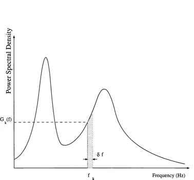
For the purpose of this thesis the spectrum is characterised by its moments as shown in Figure 2.2. Define the n-th moment of the PSD of process y[t)
/
oo Sy{uj)du) (2.31)-O O
f O O
mn = / r G ( / ) # = E (2.32)
k=i
where w (radian frequency) and / (in Hz) are frequencies, S{lo) and G{f) are double and single-sided PSDs, Mn and rrin (n = 0 ,l,...) are nth moments of the PSD, M is the total number of components in the discretised PSD, A / is the frequency interval.
Mn and m„ (n = 0,l,...) are related by
Mn = (27r)^mn (2.33)
chapter 2 27
G ,(f)
f Frequency (Hz)
chapter 2 28
From equations 2.23 and 2.32, the zeroth order moment from the spectrum gives the standard deviation of the original process. The 2nd order moment gives the standard deviation of the first order differential process.
Rice [78] and Bendat [10] worked out statistics of the spectrum. Some details related to the calculation of these statistics are shown later in this chapter. If the signal is stationary, ergodic and Gaussian, results were produced for the number of zero crossings and number of peaks per unit time.
The number of zero crossings and number of peaks per unit tim e (peak rate) are given as:
^[0] = \Jm2lmo (2.34)
E[P] = \Jm^lm2 (2.35)
Using the number of zero crossings and number of peaks, the irregularity factor
is defined as:
7 = E[0]/E[P] = m 2/\/m o m 4 (2.36)
The irregularity factor is generally taken as an indication of the frequency band width of the signal and its spectrum. It can take any value between 0.0 and 1.0. W hen 7 approaches 1.0, the signal becomes more like a regular sine wave. In this limiting case the signal is said to be narrow band and its probability density function of peaks becomes Rayleigh; cycle counting in this case is relatively easy. As the irregularity factor approaches 0.0 the signal becomes more like white noise. In this limiting case the signal is said to be completely w ide band, and its probability density function of peaks becomes Gaussian. In practice the response is rarely narrow nor completely wide band but somewhere between.
In some circumstances, the centroid of the spectrum is taken as a measurement of the frequency level of the spectrum and is defined as “mean frequency” and is made dimensionless by normalisation using the peak rate [28].