DEVELOPING A MODE CHOICE MODEL FOR MANSOURA CITY
IN EGYPT
Marwa Elharoun1, Usama Elrawy Shahdah2, Sherif M. El-Badawy3
1,2,3 Public Works Engineering Department, Faculty of Engineering, Mansoura University, Mansoura, Egypt
Received 16 October 2018; accepted 12 November 2018
Abstract: This study presents a mode choice (MC) behavioural model for individuals’ trips in Mansoura City in Egypt. Mansoura city lies in the delta region and considered as one of the most crowded cities in Egypt. The absence of effective application of urban transportation planning process in the city results in deficiencies in choosing the suitable transport policies to reduce the transportation related problems resulting from urban development and fast population increase. Mansoura does not have a transportation model; hence, developing a mode choice model for the city is considered very crucial for predicting the use of each mode, and the factors that affect selecting a specific mode. Around 10,000 online questionnaires were collected in 2015 using Google Forms. These questionnaires represent around 30,000 individual trips. In this study, only persons older than 13-years old were considered (i.e., 15,265 records). Two-thirds of the data were randomly selected and used in developing the MC model and the remaining one-third was used in validating the developed model. The developed model covers the five main modes of transportation currently employed in the city, which are Private car, Taxi, Microbus, Walking, and others. The results indicate that the developed model exhibits a good fit for the data with prediction accuracy of about 85%. Moreover, the model shows that total travel time, total cost, ownership of transport means, driving license ownership, occupational status, residence status, gender, and personal income are the main factors that significantly affect the choice of transport modes.
Keywords: mode choice, urban transportation planning, multinomial logit models, easy logit modeler (ELM), Mansoura.
2 Corresponding author: [email protected]
1. Introduction
Traditional transportation planning process has four basic steps: (1) trip generation, (2) trip distribution, (3) mode choice, and (4) traffic assignment. Trip generation determines the total number of trips produced from given origins and the total number of trips attracted by given destinations, while trip distribution estimates the trips between
Mansoura City, the capital of Al-Dakahlia governorate, is one of the largest cities in Egypt. It is the industrial, commercial, and recreational, and educational hub in the Governorate as well as the delta region. With a current population of more than one million capita as per the 2017 census (Egyptian central agency for public mobilization and statistics, 2017), Mansoura city is considered one of the most crowded cities in Egypt. The absence of effective application of urban transportation planning process in the city results in deficiencies in choosing the suitable transport policies to reduce the transportation related problems resulting from urban development and fast population increase. Mansoura does not have a transportation model; hence, one aspect that was adopted in this research is developing a mode choice model for the city, which is considered very crucial for predicting the use of each mode, and the factors that affect selecting a specific mode.
There are three main groups of factors that affect individuals’ choice of transportation modes. These groups are summarized in Ortuzar and Willumsen (2011) as follows: 1. Factors associated with the attributes of
trip maker such as age, gender, family size, car ownership and driving license ownership;
2. Factors associated with the attributes of trip such as, time of trip, and trip purpose; and
3. Factors associated with attributes of transport facilities such as travel cost, travel time and waiting time.
The MC modeling approaches can be divided into aggregate and disaggregate behavioral modeling approaches. Aggregate modeling primary focuses on the mode choices made
by average individuals for trips, while disaggregate approach concentrates on the individual choice responses as a function of the characteristics of available alternatives. It is worth noting that mode choice is usually modeled using disaggregate (i.e., discrete) choice models as it better ref lects how individuals choose a specific alternative among a set of alternatives (Ortuzar and Willumsen, 2011).
Disaggregate MC models can be classified into three main models, namely: logit models, probit models, and general extreme value models. (Ortuzar and Willumsen, 2011). The mathematical framework of these models can be found in details in (Ben-Akiva, 1974; Amemiya, 1981; Koppelman and Bhat, 2006).
In this research study, the logit model was adapted for its simple mathematical framework and its popularity among the discrete models. Logit models can be classified into two main categories: (1) binary and (2) multinomial logit models. Binary choice models can be used if the individual have only two alternatives to select from, while the multinomial logit models can be used in case of more than two alternatives (Ortuzar and Willumsen, 2011).
The discrete choice logit model is usually derived from the random utility theory. It assumes that individuals choose transport modes that maximize their utility. The utility recognized by each individual for every transportation mode is considered a random variable and can be presented as follows (Ben-Akiva and Lerman, 1985), Eq.
(1) and Eq. (2):
j A i
ij ij ij
ij k ijk k
V =
∑
θ
X (2)Where:
Uij ‒ the utility of mode i for individual j;
Vij ‒ a function of measured mode-specific
and socioeconomic variables Xijk;
εij ‒ unknown random component that
represents unobserved attributes and/or observational errors;
θk ‒ unknown calibration parameters;
Xijk ‒ the kth variable for mode j belonging to
the choice set Ai of individual i.
Multinomial Logit (MNL) model structure is probably the most widely used form of behavioral discrete choice analysis (Ben-Akiva and Lerman, 1985). It was proposed for the current analysis due to its ease of calibration and application. As well, it showed satisfactory results in many situations (Gensch, 1980).The error term (εij) for the MNL model is assumed to be
independently and identically distributed for all individuals and for each one of them as well. The mathematical structure of the MNL model is (Ben-Akiva and Lerman, 1985), Eq. (3):
exp( )
exp( )
ij ij
ik k Ai
V
p
V
∈=
∑
(3)Where:
Vij ‒ the systematic part of the utility function
of mode j for individual i;
Vik ‒ the systematic part of the utility
function of any mode k from available transportation modes for an individual i; Pij ‒ the probability of selecting mode j by an
individual i from available transportation modes;
A ‒ the set of all available transportation modes for individual i.
In logit models, the maximum likelihood (ML) method (i.e., maximization of the likelihood function) is the most popular method used for determining the unknown coefficients (Ben-Akiva and Lerman, 1985). The basic formulation of the ML method can be shown as follows, Eq. (4):
1
( , ) M
m m
L P t m
=
=
∏
(4)Where:
L ‒ the likelihood the assigned to each available alternatives;
M ‒ the total number of transportation modes alternatives;
m ‒ any alternative in the choice set; tm ‒ the observed chosen mode; and
P(tm, m) ‒ the probability for choosing
alternative m.
Instead of maximizing the likelihood function (L), the “logarithm of L” is maximized, as follows, Eq. (5):
1
og( ) M og ( , )
m
L L L P tm m
=
=
∑
(5)To better understand the relation between MC and the factors that affecting the MC behavior, many case studies have been applied around the world in the area of MC modeling. In this paper, some studies in Egypt and other similar countries are discussed.
Gharieb (2009) calibrated mode choice models to analyze the current mode choice behavior in Cairo. The study covered six modes: private car, taxi, shared taxi, minibus, metro, and public bus. They found that the factors that are affecting mode choice are gender, age, income, out of vehicle time, travel cost, and travel time. Another study in Port Said city in Egypt by El-Bany et al. (2014) showed that the factors affecting the mode choice are income, in vehicle travel time, travel cost, waiting time, and walking time.
In Palestine, two studies by A lmasri and Alraee (2013) and Abdulhaq (2016) showed that variables that affect mode choice behavior are travel time, gender, car ownership, household income, and the attitudinal variables of comfort and safety. Furthermore, another study from Saudi Arabia by Al-Ahmadi (2006) calibrated intercity disaggregate mode choice models in Saudi Arabia for three trip purposes, work and educational trips, Umrah (i.e., a type of pilgrimage made by Muslims to Mecca in Saudi Arabia), and other trips . The study cover three intercity mode choices: car, bus, and air. The results showed that in-vehicle travel time, out of pocket cost, number of family members travelling, income, trip distance, nationality of traveler, and car ownership played the important role in decisions related to intercity mode choices.
The main objective of this study is to calibrate a MC model for individuals’ trips in Mansoura City in Egypt, specifically: (1) Analyze the current situation of main mode choice by individuals in Mansoura city; (2) Determine different variables that affect the mode choice behavior of individuals in the city; and (3) Develop a reliable and accurate
model of travel mode choice for individual’s trips in Mansoura City.
To achieve the objectives of this study the work was divided into four phases. The first phase describes the study area. The second phase focused on data collection. The third phase shows a general analysis of data which focuses on the determination of travel behavior and socioeconomic characteristics. The fourth phase focused on the mode choice development. This final phase deals with calibrating and estimating of the utility functions for the model and then selecting the best MC model.
For a specified mode choice data, current estimation computer programs can be used to calibrate a MC model, such as, Biogeme (Bierlaire, 2003), SPSS (IBM Corp., 2017) and Easy Logit Modeling software (ELMWorks, Inc., 2008), etc.. In this study, the Easy Logit Modeling (ELM) software was used for its simplicity, and for its availability free of charges. With the ELM, the specification and estimation of MNL models has become practical for a much broader audience (Conrady and Jouffe, 2013).
2. Study Area
3. Data Collection
The data used in this research paper was collected using online questionnaire in Google Forms between March and July 2015. Every questionnaire represents a household. The questionnaire was divided into four sections. The first section inquires information about the residence of the respondents in the city such as (a permanent or temporary residence) and the purpose of travel to Mansoura city (studying, working or medical). The second section focuses on information about building in which the respondent lives, such as, number of households in the building, number of shops in the building, and number of workshops in the building. The third section inquires information about the family of respondent such as, family size, average family monthly income, whether the family own any transportation mean, and if yes, then how many private cars does the family own. The last section includes the set of choice alternatives consisted of ten transportation mode alternatives that are Taxi , Pickup car , Private car , Microbus , Toktok (i.e., three wheeler mode),Motorcycle , Bicycle , Work car, Walking , and any other mode of transportations. The section also inquiries about the factors that might affect the mode
choice, such as, age, gender, average monthly income, and travel cost. The responses were automatically collected using the online google spreadsheet.
A total of 10,173 online questionnaires were collected. Those questionnaires represent 35,846 individual trips. In this study only persons older than 13-years old were considered, thus only 15,256 cases were used. About two thirds of these cases were used to calibrate the MC model and the remaining data was used to validate it.
4. General Analysis of Data
The important socio-economic characteristics of trip makers such as age, gender, income, transport mean ownership and driving license were analyzed. These characteristics may identify current travel behavior of individuals in Mansoura and also define factors that may affect the choice of particular modes. The preliminary analyses of the data set are given in Table 1 and Table 2.
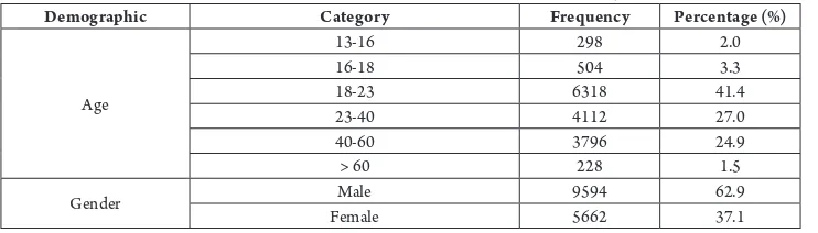
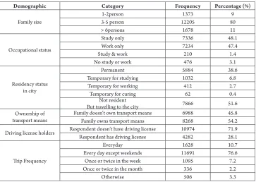
Table 1 shows the descriptive statistics of the demographic profile of individuals participated in this study, while Table 2 shows the details of the MC preference of individuals’ trips.
Table 1
Descriptive Statistics of the Demographic Profile of Individuals in Mansoura City
Demographic Category Frequency Percentage (%)
Age
13-16 298 2.0
16-18 504 3.3
18-23 6318 41.4
23-40 4112 27.0
40-60 3796 24.9
> 60 228 1.5
Demographic Category Frequency Percentage (%)
Family size
1-2person 1373 9
3-5 person 12205 80
> 6persons 1678 11
Occupational status
Study only 7336 48.1
Work only 7234 47.4
Study & work 210 1.4
No study or work 476 3.1
Residency status in city
Permanent 5884 38.6
Temporary for studying 1032 6.8
Temporary for working 412 2.7
Temporary for curing 62 0.4
Not resident
But travelling to the city 7866 51.6
Ownership of transport means
Family doesn’t own transport means 6988 45.8
Family owns transport means 8268 54.2
Driving license holders Respondent doesn’t have driving licenseRespondent has driving license 109744282 71.928.1
Trip Frequency
Everyday 1628 10.7
Every day except weekends 11691 76.6
Once or twice in the week 1095 7.2
Once or twice in the month 336 2.2
Otherwise 506 3.3
Table 2
Preference of Mode Choice of Mansoura City
Mode Frequency Percentage (%)
Taxi 2191 14.36
Pickup 103 0.68
Private car 2993 19.61
microbus 9310 61.0
Toktok 203 1.33
Otherwise 325 2.13
Bicycle 8 0.05
Work car 2 0.02
Walking 119 0.8
Motorcycle 2 0.02
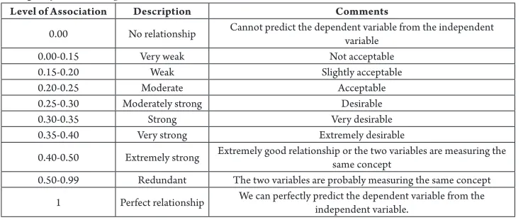
To measure the strength between the mode choice behavior and travelers socioeconomic attributes, the “CRAMER’S V” test was used. “CRAMER’S V” value varies between zero and one. If the value is close to zero it means a weak relationship between variables, while a value close to one indicates a strong relationship. Table 3 shows the strength of
“CRAMER’S V” values and hence, they have the strongest relationship with the choice of transport mode, while family size and age
have very “low Cramer’s V” value and hence they have a very weak relationship with the choice of transport mode.
Table 3
Strength of Relationship between two Variables based on “CRAMER’S V” Value
Level of Association Description Comments
0.00 No relationship Cannot predict the dependent variable from the independent variable
0.00-0.15 Very weak Not acceptable
0.15-0.20 Weak Slightly acceptable
0.20-0.25 Moderate Acceptable
0.25-0.30 Moderately strong Desirable
0.30-0.35 Strong Very desirable
0.35-0.40 Very strong Extremely desirable
0.40-0.50 Extremely strong Extremely good relationship or the two variables are measuring the same concept
0.50-0.99 Redundant The two variables are probably measuring the same concept
1 Perfect relationship We can perfectly predict the dependent variable from the independent variable.
Source: (Fletcher et al., 2018)
Table 4
Test of Relationship between the Mode Choice and Travel Socioeconomics
Factor Cramer’s V value Strength of Relationship
Gender 0.227 Moderate
Age 0.184 Weak
Family size 0.063 Very weak
Family monthly income 0.202 Moderate
Monthly personal income 0.218 Moderate
Occupational status 0.237 Moderate
Transport means ownership 0.458 Extremely strong
Driving license 0.665 Plus strong
Residence in the city 0.257 Moderately strong
Trip frequency 0.105 Weak
5. Mode Choice Model Development
The development of the mode choice model was carried out in three main steps as follows: (1) Model calibration, (2) Model validation, and (3) Sensitivity analysis. The model calibration process focuses on determining the structure of the MC model and estimating a set of parameters (i.e., coefficients) using a suitable logit model
estimation software. The calibration of the models was an iterative process. Each utility function had to be specified and then a model was calibrated. When the results were not satisfactory, the utility functions were re-specified by changing the arrangement of variables until reaching satisfactory results.
percentages of usage of transportation modes “pickup, Toktok (i.e., three wheeler mode), bicycle, work car, motorcycle, otherwise” were very low in the dataset, thus they were gathered in one mode (i.e., others). Consequently, the final modes of transportation considered in this analysis were only “taxi, private car, microbus, walking and others”. A multinomial logit model was then developed using the Easy Logit Modeling (ELM) software for calibrating the linear utility functions of the five modes using the maximum likelihood method. The list of variables that were used in model calibration with their abbreviations is presented in Table 5.
The calibrated models were evaluated using four tests. The first test was the logicality of the model variables. Each variable should appear with the expected sign indicating negative or positive impact. The second test is the statistical significance of each variable in the model. The T-statistic was used to check the significance of each variable at a 95% significance level. The
third test was the “Goodness of fit” test. The goodness of fit is represented in the ELM software by adjusted rho-square “ρ²”. Adjusted “ρ²” has a similar concept to that of the coefficient of determination (R²) in linear regression models. Adjusted ρ² value is between zero and one , where zero refers to a bad fit while one refers to a perfect fit (Koppelman and Bhat, 2006). The fourth test was the likelihood test, which was applied for comparing different models. The general test statistic for the likelihood test is as follows, Eq. (6):
-2(L(R)-L(U)) (6)
Where:
L(R) ‒ log likelihood of restricted model; L (U) ‒ log likelihood of unrestricted model.
The likelihood test statistic is asymptotically χ² distributed with (kU− kR) degrees of
freedom, where kU and kR are the number
of estimated coefficients in both models.
Table 5
Description of Explanatory Variables
Variable Description
TT Total travel time (minutes)
TC Total travel cost (L.E.)
GENDER (0 for male and 1 for female)Gender of respondent
OWTM Ownership of transport means
PINC Monthly personal income (L.E.)
WOS Occupational status
RES Residency status in Mansoura city
LICENSE Driving license holder
ASC Mode specific constant
5.1. Model Form
The first model (M1) used in this research includes only the total travel time (TT) and
between different alternatives. The private car was used as the base mode when adding constants. The utility functions for the first model (M1), initially suggested for the five modes, have the following form, Eqs. (7):
Pr .
1 2
1 2
1
1 2
( ) ( ) ( )
( ) ( ) ( )
( ) ( )
( ) ( ) ( )
Walking
ivate car
Taxi t t t t t Microbus mb mb mb mb mb
w w W
Others o o O O O
U reference mode U Asc TT TC U Asc TT TC U Asc TT
U Asc TT TC
β β
β β
β
β β
=
=
= + +
= + +
= +
+ +
(7)
The travel cost was represented by either (1) travel cost only (TC), (2) travel cost over monthly personal income (TC/PINC), or (3) travel cost over monthly household income (TC/HHINC). To choose the parameter that will be used in the model, Eqs. (7) was calibrated using the three different travel cost parameters. The Log likelihood (LL)
values at convergence for the multinomial logit models (i.e., M1) with TC, TC/PINC, and TC/HHINC were “-8376”, “-9331”, “-9881”, respectively. The model with the travel cost (TC) alone yielded the highest LL value and hence using the travel cost alone will represent a better model.
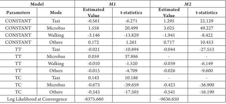
Table 6 shows the utility functions estimation for model M1. From Table 6, the estimated coefficient of travel time of “microbus mode variable has a positive sign which means that the utility of this mode decreases as the mode becomes slower which is inconvenient. The travel cost of taxi has a positive sign, which means the utility of the taxi mode increases as it becomes more expensive which is not realistic. As a result, the model M1 is therefore rejected due to the counter intuitive signs of the coefficients of some modes, and hence this leads to model M2 as shown in Table 6.
Table 6
Estimation Results of Models M1 and M2
Model M1 M2
Parameters Mode Estimated Value t-statistics Estimated Value t-statistics
CONSTANT Taxi -0.561 -6.271 1.295 22.129
CONSTANT Microbus 1.558 20.499 3.025 49.227
CONSTANT Walking -3.146 -13.829 -1.941 -8.422
CONSTANT Others 0.172 1.261 0.717 10.453
TT Taxi -0.021 -10.894 -0.044 -27.553
TT Microbus 0.059 37.886 -
-TT Walking -0.010 -1.520 -0.039 -6.149
TT Others -0.015 -4.709 -0.026 -9.600
TC Taxi 0.143 10.186 -
-TC Microbus -0.673 -39.659 -0.423 -36.900
TC Others -0.543 -17.505 -0.541 -16.190
Log Likelihood at Convergence -8375.660 -9636.650
The M2 model constants show that both travel time (TT) of “taxi, walking, and others” modes, and travel cost (TC) of “microbus, and others” modes have a large t-values which are greater than critical t-value
modes. After many iterations, a final model was obtained, as shown in Table 7. All The parameters in final model are statistically significant at the 95% confidence level. In addition, the adjusted goodness-of-fit
measures (i.e., rho-square) is 0.487 which represents a good fit.
The utility functions of modes in the final model are as follows, Eqs. (8):
private_car
microbus
U =
8.21 0.0387( ) 3.6685( ) 0.4028( ) 0.3565( ) 2.533( ) 0.8699( ) 0.0004( )
U = 9.4647 0.6567( ) 3.7778( ) 0.3154( ) + 0.4851( ) 3
t
mb
taxi
reference mode
U TT OWTM GENDER RES
LICENCE WOS PINC
TC OWTM GENDER RES
= − − + −
− − −
− − −
−
walking
others
.1763( ) + -0.7052( ) + -0.0006( ) U = 4.8674 0.0458( ) 3.4477( ) 2.9547( )
0.9238( ) 0.0003( )
U = 6.811 + 0.5721( ) 3.2569( ) + 0.4563( ) 2.8152( ) 0.2731( )
w
o
LICENCE WOS PINC TT OWTM LICENSE WOS PINC
TC OWTM RES LICENCE WOS
− − −
− −
− −
− −0.0006(PINC) 0.00356(− TTO)
(8)
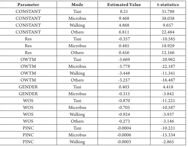
Table 7
Estimation of Final Model
Parameter Mode Estimated Value t-statistics
CONSTANT Taxi 8.21 31.788
CONSTANT Microbus 9.468 38.038
CONSTANT Walking 4.868 9.657
CONSTANT Others 6.811 22.484
Res Taxi -0.357 -10.585
Res Microbus 0.485 18.929
Res Others 0.456 12.166
OWTM Taxi -3.669 -20.962
OWTM Microbus -3.778 -22.187
OWTM Walking -3.448 -11.341
OWTM Others -3.257 -16.487
GENDER Taxi 0.403 4.418
GENDER Microbus -0.315 -3.842
WOS Taxi -0.870 -11.221
WOS Microbus -0.705 -10.587
WOS Walking -0.924 -3.937
WOS Others -0.273 -3.146
PINC Taxi -0.0004 -10.221
PINC Microbus -0.0006 -15.334
Parameter Mode Estimated Value t-statistics
PINC Others -0.0006 -9.157
LICENSE Taxi -2.533 -22.811
LICENSE Microbus -3.177 -30.054
LICENSE Walking -2.955 -8.920
LICENSE Others -2.815 -17.362
TT Taxi -0.039 -19.600
TT Walking -0.046 -7.067
TT Others -0.036 -11.468
TC Microbus -0.657 -37.401
TC Others -0.572 -18.544
Log Likelihood at Convergence -5562
5.2. The Expected Sign of Estimators
The travel time variables in the utility functions of taxi and walking modes appeared with negative signs indicating a declined utility with travel time increase. Similarly, the travel cost variables in the utility functions of microbus and others modes appeared with negative signs indicating a declined utility with cost increases. It is worth noting that the Gender appeared with a positive sign in the utility function of taxi mode, which indicates that females are expected to prefer taxi mode to private car. In contrary, the Gender appeared with negative sign in the utility function of microbus mode, which indicates that females are expected not to prefer microbus mode to private car. This agrees with the Egyptian culture. In addition, the coefficient of the “Ownership of transport mode” appeared with negative sign in the utility functions of all the transportation modes. This indicates that the use of “taxi, microbus, walking, and others” modes will decrease for individuals who own transport means. Furthermore, the monthly personal income appeared with negative sign in the utility functions of all modes. This indicates that individuals with low income are more likely to prefer other modes than private car.
For the “Residency Status” in the city, the
coefficient appeared with positive sign in the utility function of both “microbus and others” modes. This indicates that individuals who stay in the city temporarily prefer microbus and others modes more than private car. While the coefficient of “Residency Status” appeared with negative sign in the utility function of taxi mode, which indicates that individuals who stay in the city permanently prefer taxi mode to Private car. Moreover, the occupational status coefficient appeared with negative sign in the utility function of all modes, indicating that individuals who travel to the city for work or study prefer other modes to private car.
5.3. Predictive Power of the Model
by dividing the correct choices by the total number of individuals’ choices. The estimated prediction value was 0.851. In other words, the model is capable of correctly predicting about 85.1% of the choices of the trip makers. Thus, the model when used with different dataset other than the data set used for the development is still accurate.
5.4. Effect of Sample Size on Mode Choice
Modelling
It is k nown that collecting data for transportation planning in general is a tedious, time consuming, and costly process. To assess the effect of sample size on the mode choice model prediction accuracy, mode choice models were
calibrated with different sample sizes randomly selected from the data and the prediction ratio was then estimated for the 5083 events. Fig. 1 shows the prediction ratio for different sample sizes. For a sample size of 200 events, the corresponding prediction ratio is 73.20% as given in Fig. 1. As expected, the prediction accuracy increases as the sample size increases. To increase the prediction ratio by 10%, the sample size needs to be increased to 2000 observations (prediction ratio = 83.40%). It is worth noting that, from Fig. 1, by using the 10,000 observations, the prediction accuracy increased by less than 2.0% compared to the model with sample size of 2000 observations.
Fig. 1.
Effect of Sample Size on Mode Choice Accuracy
In a recent study by Habib and El-Assi (2016), the authors conducted a literature review on sample sizes of recent household travel surveys around the world. They found that the sample size used in recent studies in the USA ranged between 0.11% and 1.0% of households (7 studies with an average sample
size of 0.41%). While in Canada, the sample size was larger and ranged between 2.20% and 5.0% of households (8 studies with an average sample size of 3.88%).
observations), the prediction accuracy is about 84.50%. It is worth noting that using larger size samples will have slight improvement on the prediction accuracy as shown from Fig. 1. Furthermore, to achieve 80 % prediction accuracy only 870 observations are required to calibrate the mode choice model. In fact, the 80% prediction accuracy can be considered as a preferable accuracy when calibrating a mode choice model for similar cities to Mansoura.
5.5. Mode Choice Model Stability
The data used to calibrate the MC model was collected in 2015. Nevertheless, by the end of 2016, the Egyptian central bank floated the currency, and later on by the end of June of 2017, the Egyptian government increased the fuel prices by about 35% to 47% for different fuel types. Hence, the travel cost of all the transportation modes increased significantly. This of course is expected to affect the individuals’ behavior when choosing between different transportation modes. For this purpose, another 100 questionnaires, which represent 380 observations for persons older than 13 years, were collected during the period between December 2017 and January of 2018 by personal interview survey.
The final MC model (Eqs. (8)) was used to check the prediction accuracy of the new 380 individuals to check the stability of the MC model with variables changes. The estimated prediction value was 0.846, which means that the model that was calibrated based on the 2015 data is capable of predicting about 84.60% of the choices of the trip makers for the new data. This shows the stability of the model and that it is still appropriate in predicating the mode choice behavior for individuals despite the change in the travel cost. It is worth noting that the Egyptian
government increased the fuel prices again in June 2018, but the effect of the new fuel prices and their subsequent effect on travel costs were not checked in this research.
5.6. Sensitivity Analysis of Increasing
Microbus Fare
As the Egyptian government is expected to re-reduce subsidy on fuel and other public transit fare, it is worth checking the sensitivity of increasing the microbus fare. The effect of increasing travel cost of microbus on modal shares of other modes was checked using 25%, 50%, 75%, 100%, and 125% increase of microbus fare given that all other variables were held constant to observe the varying percentage modal split for all travelling modes with a change in the value of the microbus fare increase.
Fig. 2 show the effect of increasing travel cost of microbus on mode shares. From Fig. 2, by increasing the microbus fare the probability of using the microbus decreases. For example, the probability of using the microbus decreased by 30% (i.e., 50% of its current share) when the fare increased by 100%. In addition, the probability of using the private car and taxi slightly increased when the microbus fare increased (e.g., less than 3% increase for 100% microbus fare increase).
Fig. 2.
Effect of Increasing Travel Cost of Microbus
6. Summary and Conclusions
This study presents a multinomial mode choice (MC) logit behavioural model for individuals’ trips in Mansoura City in Egypt. Around 10,000 online questionnaires representing 30,000 individual trips were collected in 2015. The total data points of 15265 records were used for the model development and validation. Two-thirds of the data were randomly selected and used in developing the MC model and the remaining one-third was used model validation. The developed model covers the main five modes of transportation in the city, which are Private car, Taxi, Microbus, Walking, and others. The following conclusions were drawn:
• The factors significantly affect the choice of transport modes were found to be the total travel time, total cost, ownership of transport means, driving license ownership, occupational status, residence status, gender, and personal income;
• The developed model ex hibits a good fit for the data with prediction accuracy of about 85%. Furthermore,
the prediction accuracy of the model that was calibrated using the 2015 data was rechecked using data from 2017 and 2018 and the model prediction ability was still good;
• Using sample sizes larger than 2000 observations would slight improve the prediction accuracy. In addition, to achieve at least 80% prediction accuracy, only 870 observations will be required;
• The probability of using microbus will decrease by increasing the microbus fare, while the probability of using private car and taxi will slightly increase by only about 2% for 100% increase in microbus fare. In addition, it was found that the increase in microbus fare would increase the probability of people walking and using other modes rather than taxi and private car.
Acknowledgment
References
Abdulhaq, D.M.N. 2016. Transportation Mode Choice Model for Palestinian Universities Students: A Case Study on An-Najah New Campus, Master of Science thesis, An-Najah National University-Faculty of Graduate Studies.
Al-Ahmadi, H.M. 2006. Development of intercity mode choice models for Saudi Arabia, Engineering Sciences 17(1): 3-12.
Almasri, E.; Alraee, S. 2013. Factors Affecting Mode Choice of Work Trips in Developing Cities—Gaza as a Case Study, Journal of Transportation Technologies 3(04): 247-259.
Amemiya, T. 1981. Qualitative response models: A survey, Journal of Economic Literature 19(4): 1483-1536.
Ben-Akiva, M. 1974. Structure of Passenger Travel Demand Models, Transportation Research Record 526: 26-42.
Ben-Akiva, M.E.; Lerman, S.R. 1985. Discrete choice analysis: theory and application to travel demand (Vol. 9). MIT press.
Bierlaire, M. 2003. BIOGEME: a Free Package for The Estimation of Discrete Choice Models. In Proceedings of the Swiss Transport Research Conference, No. TRANSP-OR-CONF-2006-048.
Conrady, S.; Jouffe, L. 2013. Modeling Vehicle Choice and Simulating Market Share with Bayesian Networks: A case study about predicting the U.S. market share of the Porsche Panamera using the Bayesia Market Simulator. Available from internet: <https://library. bayesia.com/download/attachments/4882677/choice_ modeling_v32.pdf>.
Egyptian central agency for public mobilization and statistics. 2017. Egyptian Population in 2017 [in Arabic]. Available from internet: <http://www.capmas.gov.eg/ Admin/Pages%20Files/201871611358gov.pdf>.
El-Bany, M.E.S.; Shahin, M.M.; Hashim, I.H.; Serag, M.S. 2014. Policy Sensitive Mode Choice Analysis of Port-Said City, Egypt, Alexandria Engineering Journal 53(4): 891-901.
El Esawey, M.; Ghareib, A. 2009. Analysis of Mode Choice Behavior in Greater Cairo Region. In Proceeding of the 88th Annual Meeting of Transportation Research Board,
No. 09-0168.
ELMWorks, Inc. 2008. Easy Logit Modeling (ELM) Software, Version 1.1.10 [Computer Software]. Available from internet: <http://elm.newman.me>.
Fletcher, J.; Ramanathan, T.; Dallaire, S.; Szala, M.; Saini, A.; Levine, R. 2018. POL242 Online Lab Manual, University of Toronto. Available from internet: <http:// www.chass.utoronto.ca/~josephf/pol242/onlinetutorials. htm>.
Gensch, D.H. 1980. Choice model calibrated on current behavior predicts public response to new policies,
Transportation Research Part A: General 14(2): 137-142.
Habib, K.; El-Assi, W. 2016. How Large is too Large? The Issue of Sample Size Requirements of Regional Household Travel Surveys, the Case of the Transportation Tomorrow Survey in the Greater Toronto and Hamilton Area. In Proceeding of the 95th Annual Meeting of Transportation Research Board.
IBM Corp. 2017. Released 2017. IBM SPSS Statistics for Windows, Version 25.0. [Computer Software].
Koppelman, F.S.; Bhat, C. 2006. A self-instructing course in mode choice modeling: multinomial and nested logit models. U.S. Department of Transport, Federal Transit Administration. Available from internet: <http://www. caee.utexas.edu>.
Ortuzar, J.; Willumsen, L.G. 2011. Modelling transport. John Wiley & Sons. 607 p.
Richardson, A.J. 2003. Creative Thinking About Transportation Planning. In Proceeding of the 82nd Annual