www.nat-hazards-earth-syst-sci.net/14/1491/2014/ doi:10.5194/nhess-14-1491-2014
© Author(s) 2014. CC Attribution 3.0 License.
Forecasting wind-driven wildfires using an inverse modelling
approach
O. Rios1, W. Jahn2, and G. Rein3
1Centre for Studies on Technological Risk (CERTEC), Universitat Politècnica de Catalunya, Av. Diagonal, 647, 08028 Barcelona, Spain
2Departamento de Ingeniería Mecánica y Metalúrgica, Pontificia Universidad Católica de Chile, Santiago, Chile 3Department of Mechanical Engineering, Imperial College London, SW72AZ, London, UK
Correspondence to: G. Rein ([email protected])
Received: 30 September 2013 – Published in Nat. Hazards Earth Syst. Sci. Discuss.: 4 December 2013 Revised: 10 April 2014 – Accepted: 15 April 2014 – Published: 13 June 2014
Abstract. A technology able to rapidly forecast wildfire dy-namics would lead to a paradigm shift in the response to emergencies, providing the Fire Service with essential in-formation about the ongoing fire. This paper presents and explores a novel methodology to forecast wildfire dynamics in wind-driven conditions, using real-time data assimilation and inverse modelling. The forecasting algorithm combines Rothermel’s rate of spread theory with a perimeter expansion model based on Huygens principle and solves the optimisa-tion problem with a tangent linear approach and forward au-tomatic differentiation. Its potential is investigated using syn-thetic data and evaluated in different wildfire scenarios. The results show the capacity of the method to quickly predict the location of the fire front with a positive lead time (ahead of the event) in the order of 10 min for a spatial scale of 100 m. The greatest strengths of our method are lightness, speed and flexibility. We specifically tailor the forecast to be efficient and computationally cheap so it can be used in mobile sys-tems for field deployment and operativeness. Thus, we put emphasis on producing a positive lead time and the means to maximise it.
1 Towards an operative forecasting tool
Current computational wildfire dynamics simulators are not fast enough to provide valid predictions on time (Sullivan, 2009) and require input parameters that are difficult to ac-quire and sense during an emergency situation. A potential solution to develop an operational forecasting tool is to
as-similate real-time sensor data (Cowlard et al., 2010), which has been shown to greatly accelerate fire simulations without loss of accuracy (Mandel et al., 2008; Jahn et al., 2011; Ro-choux et al., 2013). The cornerstone to reach such a tool is to find a computational algorithm that combines a fire model with sensor data that reliably delivers an accurate forecast with a positive lead time (i.e. time before the event, in the order of 10 min for a spacial scale of 100 m), and enables emergency responders to make better tactical decisions. At the same time, it has to be versatile enough to be adapted in different fire situations (range of fuels, complex topogra-phy, weather conditions). Ideally, it should also be able to in-corporate the effect of fire fighting actions (e.g. water lines, fire breaks, back fires) and weather forecasts. More impor-tantly, it should not require high computational resources (i.e. high-performance computing or supercomputers) so that it can also be deployed flexibly in portable devices by fire re-sponders.
1.1 Data assimilation and inverse modelling
The inverse method is particularly appropriate for wildfire modelling due to the large amount of unknowns. The fuel properties, location, area covered by foliage, moisture con-tent, meteorological conditions and topography are necessary parameters to initialise a fire model but all of them can hardly ever be measured. By contrast, the inverse approach can find these parameter by using a range of sensor measurements of the ongoing fire.
Despite its promising capacity for coping with complex problems with a large number of unknown parameters, only few authors have tried to apply data assimilation or forecast-ing techniques to fire science. Among these, Jahn et al. (2011, 2012) successfully pioneered the approach to forecast fires in enclosures using both simple and complex models (two-zone model and computational fluid dynamics). In the field of wildfire, Mandel et al. (2009) explored this technique to predict the time–temperature curve of a sensor placed in the way of an advancing wildfire. They examined a reaction– diffusion equation and a semi-empirical fire line propaga-tion model coupled with an Eulerian level-set-based equa-tion. Despite this progress, their implementation was found to be unstable due to the generation of spurious fires which cause non-physical results.
Rochoux et al. (2013) pioneered the successful application of data assimilation to predict the location and spread of the wildfire front using infra-red sensors. Data were assimilated with a Kalman filter to balance computational and sensor er-rors. Rochoux et al. (2013) assimilates perimeter locations at different times and uses the fuel depth as the only input. The propagating model uses two components: the rate of spread (RoS) is represented by a product between the fuel depth (δ) and a constant (0) to be quantified as part of the forecasting problem (RoS=0·δ). Their model uses a level-set-based equation to cast the fire perimeter. They tested the model in a controlled small-scale experiment assimilating one fire front and delivering a 30 s forecast. Most recently, Rochoux et al. (2014) have presented a work that solves for more than one parameter and uses parallel computing. Also using a level-set model and sensor data, Lautenberger (2013) ex-plored stochastic optimisation of the wildfire problem. Coen et al. (2013) used satellite data to initialise a weather–wildfire growth model at the kilometre scale.
The greatest strengths of our method presented here are lightness, speed and flexibility. We specifically tailor the forecast to be efficient and computationally cheap so it can be used in mobile systems for field deployment. Thus, we put emphasis on producing a positive lead time and the means to maximise it, while at the same time solving for multiple pa-rameters. These are not the objectives of other papers in the literature. For example, Rochoux et al. (2013), the truly first paper in the literature that effectively forecast wildfire be-haviour, integrates measurement errors with model errors to increase accuracy (standard procedure in weather forecast-ing), but it comes at the price of higher computational ex-pense. Rochoux et al. (2013) and Mandel et al. (2008) use
one single parameter at a time and do not emphasize lead times. Moreover, they seem tailored more towards supercom-puting platforms than to mobile systems for field deploy-ment.
Another highlight of our method is the incorporation of automatic differentiation into the inverse model, which is ac-curate and fast, further decreasing the computational expense of a forecast.
1.2 Forecasting algorithm
We formulate the inverse problem based on the premise that some invariant exists by following the contributions of Jahn et al. (2012) on forecasting fire dynamics in enclosures. We define the invariants as the set of governing parameters that are mutually independent and constant for a significant amount of time. Invariant is a concept already in the liter-ature (Jahn et al., 2012). Therefore, our implementation re-lies on the assumption that some physical attributes of the system remain constant at least during some time. Those at-tributes can be uniform, a scalar or a vector field with spatial dependency. From the point of view of our methodology, in-variants are a central concept to forecasting systems that do not focus on the initial conditions only. For example, weather forecasting (i.e. Coen et al., 2013) solves an inverse problem to find the initial conditions, and then runs the forward model for predictions. In our work, we solve the inverse model of selected key parameters inside the governing equations, the invariants, not the initial conditions. It is an essential prop-erty of the invariants that they remain constant during the lead time of the forecast. When any invariant changes signif-icantly (e.g. due to divergence of the assumptions or external conditions) its effect is to limit the lead time. Examples of such quantity are initial fuel’s moisture content or fuel depth. However, the invariants are not restricted to physical vari-ables but can represent mathematical attributes of the system as well. For instance, if the wind speed changes but its ef-fect on the RoS remains constant (boundary layer regime is maintained) the most important invariant will be its effect on the rate of spread rather than the wind speed itself.
After assimilating data during a period of time (assimila-tion window) the invariants are estimated and used to fore-cast the perimeter evolution. This forefore-cast is then accurate until any of the invariants change significantly, which would be detected with the help of the continuous data feed from sensors. The sensor errors in the assimilated data are con-sidered to be smaller than the model accuracy and therefore their influence is not directly considered here. This is a com-plementary approach to that of Rochoux et al. (2013) who balance data errors with model errors.
However, additional data such as flame height or spread-ing rate (recently measured by infra-red images and stereo vision; Rossi et al., 2013) could be considered in future de-velopments.
2 Building up the forward model
The initial step when posing an inverse modelling problem is to determine the forward model and its invariants. The for-ward model is the set of equations that relates the invariants to the observables (variables that can be measured with sen-sors). Its importance in the is twofold: the forward model is first used iteratively to quantify the invariants and then run again to deliver a forecast valid until the invariants change or the next assimilation process is started.
To create our forward model, we combined Rothermel (1972) and Richards (1990) models. The Rothermel model estimates the RoS of any point in the fire front whereas the Richard model uses these RoS to generate the elliptical firelets that expand the fire front and compute its location at any time.
2.1 Rothermel’s model
Rothermel’s model is based on an energy balance equation where the heat sources and sinks are identified to estimate the RoS of a surface fire. The original model uses several empirical correlations from wind-tunnel experiments for fires spreading at quasi-steady state. This means that any acceler-ation of the fire is not considered. The shape of the fire front is assumed to have no influence on the RoS.
Rothermel’s equation can be recast with three invariants (Ix), defined as follows:
RoS=Imf(1+Iu·Iw). (1)
Imf captures the effect of all the fuel properties; ovendry fuel loading (wo), surface-area-to-volume ratio (σ), moisture content (Mf), moisture of extinction (Mx) and fuel depth (δ):
Imf=F(σ, wo, δ, Mf, Mx). (2)
The wind speed is directly equal toIu:
Iu=U. (3)
The effect of the wind speed on the fire spread also de-pends on fuel properties such as layout, bulk density, surface-area to volume ratio and fuel depth. Its effect is embedded in
Iwas
Iw=K(σ, wo, δ)·UB−1, (4)
whereBis an empirical coefficient.
2.2 Huygens principle
Although Rothermel’s model can estimate the RoS of any point, it is a mean value for the head fire (Rothermel, 1972) and does not inform about different directions of spread. Therefore, it is not sufficient in predicting the fire front shape and location. In parallel to RoS estimation, some other model must be used to represent the fire perimeter expansion. We used Huygens’ principle – originally postulated to explain light wavefront propagation – with elliptical expansion, as proposed by Richards (1993). Applying it to wildfire, this principle considers every point in the fire perimeter at time
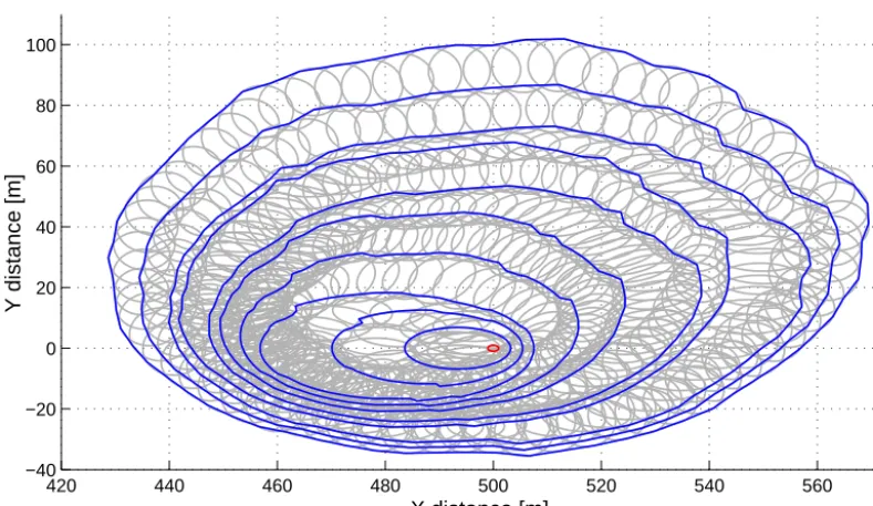
t as a new ignition source that spreads during a time dt fol-lowing an elliptical template shape – known as a firelet. The corresponding fire front line at timet+dtis the outer curve that envelopes the firelets centred on the rear focus as shown in Fig. 1.
The details of the Huygens firelet model can be found in Richards (1990, 1993), but an overview of the main concepts and equations is provided here.
Considering the initial ignition point situated at{X0, Y0} and using a parametrisation variable s∈ [0−2π], the
{(xi(t ), yi(t )}coordinates of fire front vertices can be ana-lytically calculated by integrating a set of partial differential equations:
x(s,t )ˆ =X0+
ˆ
t
Z
0
a2(t )cosθ (t )cos(K)+b2(t )sinθ (t )sin(K)
q
a2(t )cos2(K)+b2(t )sin2(K)
·c(t )sinθ (t )
dt (5)
y(s,t )ˆ =Y0+ ˆ t Z
0
a2(t )sinθ (t )cos(K)+b2(t )cosθ (t )sin(K) p
a2(t )cos2(K)+b2(t )sin2(K) ·c(t )cosθ (t ) !
dt, (6)
where
K=θ (t )+s, (7)
whereθis the wind direction andbandcare related to the backwards and to the forward propagation velocities that can vary spatially and are calculated by imposing Rothermel’s rate of spread for the head fire from the new ignition point:
b(s, t )+c(s, t )≡RoS(s, t ). (8)
The lateral front velocitya, however, is directly related to the eccentricity of the firelet. It was originally estimated using an experimental correlation found by Anderson (1983) that relates the ratio between the major and the minor firelet’s axis, and thus, the ratio betweenbanda(independent of the time step1tused). Its value depends on the wind speed (U) in accordance with the equation
a(s, t )
b(s, t )=0.936e
0.2566U+0.461e−0.1548U−0.397≡LB. (9)
420 440 460 480 500 520 540 560 −40
−20 0 20 40 60 80 100
Y distance [m]
X distance [m]
Figure 1. Example of Huygens expansion with elliptical firelets (grey lines) from an ignition point (red dot in the centre). Ten fire fronts
(blue lines) are plotted during the spread of the fire over an heterogeneous fuel depth (0.6±0.3 m) and under changing wind (5±2 m s−1) speed and direction at every time step (1 min each). This Rothermel–Huygens model is also used in FARSITE (Finney, 1998).
constant 0.397 is a modification of Anderson’s original for-mula to ensure that the fire expands circularly (LB=1) un-der no-wind conditions (U=0).
Once the LB, a,b, c velocities can be calculated using Eqs. (8) and (9) and the elliptical geometry properties:
a=RoS1+1/HB
2LB (10)
b=RoS1+1/HB
2 (11)
c=b−RoS
HB, (12)
where HB= LB+
p
LB2−1 LB−
√
LB2−1.
If the invariantIu=U, introduced in Rothermel’s model, is reused in Huygens’ firelets expansion, only one additional invariant is required to account for the principal direction of spreading determined by the wind direction:
Iθ=θ. (13)
The forward model is then a function of four invariants:
M(Iu, Iw, Imf, Iθ, T )=
(
RoS=R(Iu, Iw, Imf)
{x, y} =H(RoS, Iu, Iθ, T ), (14) where T is the time when the latest sensor data arrive, R
represents Rothermel’s model with cast invariants (Eq. 1) and
Hthe firelet expansion (from Eqs. 5 and 6).
Depending on the available sensor data, the invariants can be turned into input data for the problem. For example, if reliable wind speed data arrive, there is no need to solve for it but instead it is directly used as input in the forward model. 2.3 Cost function
The invariants are calculated by minimising a cost function
J that measures the difference between the model output and the sensor observations. The cost function proposed is the Euclidean norm summed over the different assimilation times:
J(p)=
tf X
t=ti q
xi− ˆxi(p)TWixi− ˆxi(p), (15)
where{xi} ∈R2are theN-coordinate set of the observed fire
front position in a given time stepiandxˆi(p)=Mx(p)are the corresponding model output positions for a set of invari-ants (p). Wi is a weigh function that could be used to give more importance to particular sets of sensor data. However, in the present work no weighting function is used (Wi=
I) but the framework is set to allow introductions of
Equation (15) can be simplified if thex–ycoordinates are concatenated as one-row vectoryi andy˜i=Mi(p):
J(p)=
tf X
t=ti q
yi− ˜yi(p) T
yi− ˜yi(p). (16)
Although the square root gives the correct Euclidean norm, it does not affect the minimisation and therefore was re-moved for the computational implementation. Each observed front (yi) is angularly discretised between rays emanating from the origin of coordinates. The model output (y˜i) is also angularly discretised at each optimisation step, so a La-grangian framework is used and updated for the evaluation of the cost function. No refinement is added regarding the front convexity, although this could be explored in further versions of the work to handle more complex front shapes.
2.4 Optimisation
There are two main approaches to minimise Eq. (16): gradient-free or gradient-based (Nocedal and Wright, 1999). The first group are stochastic algorithms that evaluate the cost function J(p) at many points to find the absolute minimum, whereas the second group use an initial guess (pb) and follow the gradient direction towards the clos-est minimum. Although gradient-free algorithms can sweep a broader search space to find the absolute minimum, they have to evaluate the cost function multiple times which is computationally expensive if the forward model is slow. On the other hand, when the cost function is continuous and the possible range of values of the invariants(p)is known as it is in our problem), the gradient-based algorithms are more suit-able and efficient. Gradient-based algorithms can converge to a local minima instead of a global one. However, the ex-tended sensitivity analysis performed on our problem showed that the system is benign in the sense that all the functions in-volved behave smoothly.
If the forward modelJ(p)is linear then the cost function is quadratic and can be minimised by solving a system of linear equations (as will be shown in the following sections). For forward models that are not linear – as is the case – the tangent linear model (TLM) is used for local linearisation (Griewank, 2000).
2.5 Tangent linear model
The TLM consists in linearising the forward modelM(p)in the vicinity of an initial guesspb. This linearisation can be done if the model is weakly nonlinear, as in this case. The vi-ability of the TLM relies on the initial guess and the fact that the procedure is iterated until convergence. To calculate the TLM we use first-order Taylor series expansion aroundpb.
The gradient of the linearised function is then
∇pJ(p)=2
tf X
t=ti h
∇pMi(pb)(p−pb)
iT
(17)
h
yi−Mi(pb)+ ∇pMi(pb)(p−pb)
i
.
Applying the first-order condition for minimisation and in-troducing the following notation:
Mi=Mi(pb) Hi = ∇pMi(pb)
pi=(p−pb)
gives tf X
t=ti
HTiHip= tf X
t=ti
HTi(yi−Mi), (18)
which is a linear system that can be easily solved by us-ing a QR factorisation with column pivotus-ing (Nocedal and Wright, 1999).
2.6 Automatic differentiation
Calculating the Jacobian multiplication term HTiHi in Eq. (18) requires partially differentiating the model with re-spect to the different invariants. This has to be donep×2n× mtimes, wherepis the number of invariants used, 2nthe co-ordinates of the fire front andmis the number of times that data arrives during the assimilation window..
The simplest way to numerically evaluate the Jacobian is by finite centred differences:
Hjk,i=∂M
j i(pb)
∂pk
'M
j i p
b+
k−Mi(pb)
||k||
,
wherek∈Rp= {0,0, . . . , . . .0}is a small perturbation of
magnitudein the positionk.
But this approach has two downsides: the forward model has to be evaluated twice each time, andshould be reduced as much as possible which introduces numerical truncation errors (Griewank, 2000). For these reasons, we discarded fi-nite differences and chose an automatic differentiation ap-proach.
Automatic differentiation allows to directly calculate the Jacobian matrix Hi (normally called Tangent Linear or For-ward) or HTi (called Adjoint). It consists of iteratively apply-ing the chain rule of differential calculus to the programmapply-ing code of the forward model and so obtain directly the code for all the partial derivatives.
!"#
$%#
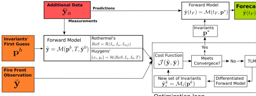
Figure 2. Program structure flow diagram. Orange boxes are the required inputs, green box is the output and red box shows additional inputs.
The tangent linear differentiation is preferable when the number of observables 2n(i.e. model outputs) is much larger than the number of invariantsp. By contrast, calculating the adjoint differentiation is more convenient and efficient when there is a large number of invariants. Therefore, in the present work, we use tangent linear differentiation.
In future work, if the number of invariants is increased, the Adjoint Automatic Differentiation should be explored to keep the computational efficiency high and maximise the lead time.
2.7 Structure of forecasting algorithm
Figure 2 summarises the principal parts of the assimilating and inverse modelling program.
First, fire front positionsyare assimilated during a specific period of time (called assimilation windows). Meanwhile, an educated guess estimates the first set of invariantspb. This first guess is based on roughly estimated data. Its influence on the model is explored in Sect. 3.1. This invariant guess is input into the forward model together with the timeT of the last sensor data arrival and one known fire front position (or the initial ignition point)M(pb, T ,y0). The consequent first prediction set of frontsy˜i is compared with the assimilated data by means of the cost function J(y˜−y)(see Eq. 16). If the the cost function is not zero, the algorithm starts the optimisation loop.
The first statement in the loop is to calculate the Jacobian terms in Eq. (16). The output is a new set of values for in-variantspk that is input to the forward model to get a new estimated set of fire fronts. If the convergence criteria are met, then the best estimated invariants vector has been found (p∗) and thus the forecast is delivered by running the for-ward model at until the forecast timetF. Otherwise, the loop is iterated again.
The fact that a loop is needed to estimate the invariants reduces the inaccuracy added by applying a tangent linear approach to a nonlinear model since in every new iteration the model is linearised (i.e. the differentiated forward model is run) in a new state point (pk+1). In addition, if any of the new invariant values in the vectorpk+1exceeds the physical range, its value is set back to the initial guess to prevent non-physical results.
Note that every time that the differentiated forward model is run, the forward model is also evaluated. Thus the forward model is always evaluated at the same time as the differenti-ated model, speeding up the algorithm and enabling the use of complex forwards models that would be prohibitive with a finite differences approach.
Regarding convergence, two criteria can be requested. The first is to state a maximum allowable error for the predictions via the cost function. The second is to state a maximum al-lowable change between consecutive invariant vectors. While the first criterion ensures the predictions match the observa-tions, the second criteria might not always do so. In the fol-lowing sections, both criteria are explored and compared. 2.8 Synthetic data
460 480 500 520 540 560 580 600 −40
−20 0 20 40 60 80 100 120 140
xdistance [m]
ydistance [m]
1st guess iteration 1 iteration 2 iteration 3
Figure 3. Guess, observation and iterations of fire fronts in anx–yplane (plan view of a wildfire). The black triangles are the 15 observed perimeters. The red dashed lines are the fire fronts generated with the first guess and the dashed lines are the following iterations. The last iteration is the green solid lines.
3 Results
The performance of the forecasting algorithm is investigated in different situations where synthetic data simulate the ob-servations to assimilate. The tests are performed for different values of parameters like the assimilation window, assimi-lated data (fire fronts locations and feeding frequency) and initial guess. We look at several features like convergence of the invariants, minimisation of the cost function, effect of the initial guess, effect of the assimilating window width, the computing time and the leading times obtained.
The same methodology is also applied with alternative in-variants to handle situations where some of the quantities as-sumed as constant are allowed to vary.
In all of the following tests, punctual ignition source is considered as the initial integration point for the fire front expansion. This ignition point source is depicted as a red spot in all the plots and is a required piece of information to run the forecasting algorithm. In a real wildfire situation, it could be identified as the first reported location of the fire. If the fire has spread out before the first bit of information arrives and it is no longer a point source, the first assimilated fire front can be also used as a virtual ignition perimeter by considering the whole fire front as a set of initial ignition sources.
3.1 Initial guess
The forecasting algorithm needs an initial guess of the invari-ant value where the first tangent linear approximation (TLM) is performed. This first educated guess can be directly gener-ated within the range of validity of each invariant – without considering any hint from the actual wildfire – or by using Rothermel equivalent equations (Eqs. 2–4 and 13) and esti-mating the six physical underlying quantitiesδ,Mf,Mx,σ,
W0andθwhich can be roughly done by observing the fuel and wind.
The six initialising quantities were studied over the range of values found according to operational-based considera-tions. For instance, the fuel depth δ can be easily distin-guished to be between 5 cm pine needle litter or 1 m for tall grass. Its offset of the initial guess is lower than 1.50 m. In contrast, some other variables such as moisture content (Mmf) or ovendry fuel loading (wo), cannot be estimated with such easy and therefore the possible offset is much larger. 3.2 Quantifying the invariants
1st guest−50 1 2 3 −30
−10 10 30 50
off−set true vlaue [%]
# Iterations
1st guest 1 2
0 5000
Cost Function Value [m
2]
I
u Iθ Iw Imf Cost
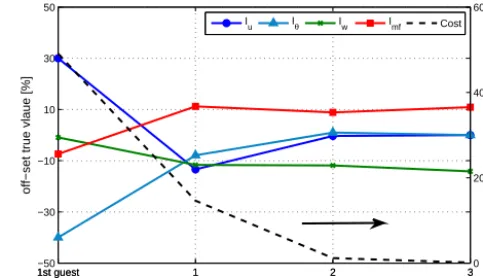
Figure 4. Convergence of cost function (dashed line, right axis) and
individual convergence of each invariant to the true value (solid lines, left axis) as a percentage difference. Assimilation windows
=15 min (1 assimilation min−1).
a rapid decrease towards zero. Its slope quantifies the con-vergence rate. At the first iteration the slope is steep which indicates that the algorithm quickly corrects the large dis-crepancies. As the cost decreases so does the slope, indicat-ing that convergence is achieved. Fig. 4 also shows that all invariants converge to the true values with 2 % of difference. 3.3 Invariant Multiplicity
The window width (WW) is the length of time during which the forecasting algorithm is being fed data (i.e. fire front lo-cation in the case at hand). The time between consecutive fire front observations is called assimilation period (1T) and can be directly related to the assimilating frequency (F =1/1T).
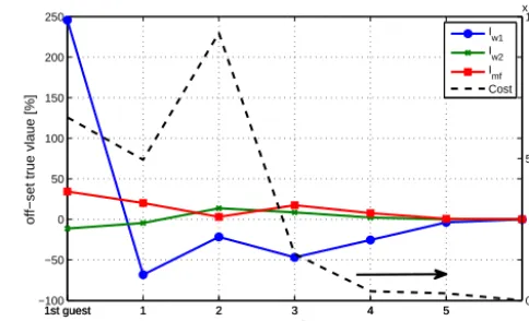
The main effect of the number of assimilated fronts (WW/1T) is resolving the problem of invariant multiplic-ity (or interdependence). Multiplicmultiplic-ity is when different val-ues of two or more invariants lead to the same prediction of the fire perimeter. The value of the cost function tends to in-crease as the assimilation window inin-creases and more fronts are assimilated. The error of the initial guess amplifies with the propagation (the previous fire front position is required to calculate the new one) and therefore the forecasting algo-rithm is more sensitive to the wrong identification of invari-ants. This is shown in Fig. 5 where instead of assimilating 15 min (and 15 fire fronts) – as in the converging example Fig. 4 – we assimilate front positions during 3 min (i.e. three front positions). The cost function rapidly drops to zero but in this case the value estimated for both ImfandIw differs from the true value by 10 %. The reason is that now the ini-tial cost function has a lower absolute value since the prop-agation of an inaccurate estimation is truncated in time and therefore the effects of an incorrect assimilation are hidden. It is worth mentioning that despite the possibility ofImfand
Iwmisconverging, RoS is always correctly estimated as it has
1st guest 1 2 3
−50 −30 −10 10 30 50
off−set true vlaue [%]
# Iterations
1st guest 1 2 30
200 400 600
Cost Function Value [m
2]
I
u Iθ Iw Imf Cost
Figure 5. Convergence of cost function (dashed line, right axis) and
individual convergence of each invariant to true value (solid line, left axis). Assimilation windows=3 min (1 assimilation min−1).
no multiplicity in the forward model and only one value can fit the observations.
One way to deal with multiplicity is by defining only one invariant for the RoS. This approach, however, does not al-low for the forecasting algorithm to be ameliorated if extra data become available (as will be done in Sect. 3.5) since no information about particular contributions is achieved. Thus, a more interesting way to diminish multiplicity is to recast the invariants and input extra data in a way that they become functionally independent. For instance, if the fuel–moisture invariant is multiplied by a measurable quantity (such as fuel depth or moisture content) that varies spatially or over time, then its value is no longer exchangeable with the wind fac-tor. The same strategy could be used for the wind invariant if wind speed is known. This approach is successfully explored in the following sections.
The third way to deal with multiplicity is by assimilating additional quantities that are predicted by the forward model. It is worth pointing out the difference between inputting addi-tional values and assimilating more data. The first consists of extra inputs to run the forward model and allows it to handle more complex situations. Examples of this could be informa-tion of moisture content, fuel properties or wind speed. More data assimilation, in contrast, requires more outputs from the forward model. Thus, in our case, only the positions of the fronts are assimilated but the forward model can be comple-mented so it delivers additional characteristics such as flame height or fire intensity. By assimilating this additional data the invariant multiplicity is reduced since each invariant is then part of different equations and they are no longer de-pendent.
3.4 Positive lead times
4 8 12 16 20 24 0
5 10 15 20 25
Number of assimiated fronts
Computing Time [s]
10 min forecast 20 min forecast 30 min forecast 40 min forecast
Figure 6. Computing time required for four different forecasting
time lengths (10, 20, 30 and 40 min) versus the number of assimi-lated fire fronts.
lead time is defined as the amount of time between the deliv-ery of the forecast and the successful predicted event. If the forecasting algorithm needs 25 s of computing time to deliver a 10 min forecast, then the lead time is 9.6 min. As shown in Fig. 6, the model is so fast (in the range from 2 to 25 s) that it delivers always a positive lead time in the order of dozens of minutes for the case of synthetic data.
The lead time principally depends on the number of as-similated fronts and the initial guess (i.e. iterations required for convergence). The forecasting time lengthtF(either we ask for a 10 min or 40 min forecast) also plays a role when the forward model is computationally demanding. However, due to the synthetic data scenario used in the case at hand, its contribution is limited as shown in Fig. 6.
3.5 Different data contexts
The invariants can be adapted to different data situations. To show the versatility of our model two different cases with different available data are presented as example.
In the first case, wind speed and direction are provided and assumed to be uniform – same wind speed and direction for all the fire perimeter – although they can vary in time. By contrast, in the second case, the fuel depthδis provided as as sensor data and is allowed to vary spatially. Wind speed and direction can be gathered from deployed units as well as from weather stations. Regarding the information about fuel, for-est managers usually map forfor-est areas in advance to list their spatially distributed characteristics. New techniques recently brought into the field such as the use of lidar – light detec-tion and ranging (Mutlu et al., 2008), potentially increases the accuracy and availability of this information and opens the door for preparing operative measuring systems for the situations when these data are not known.
1st guest 1 2 3 4 5
−100 −50 0 50 100 150 200 250
off−set true vlaue [%]
# Iterations
1st guest 1 2 3 4 5 0
5 10 x 104
Cost Function Value [m
2]
I w1 I
w2 I
mf Cost
Figure 7. Convergence of the cost function and the invariants when
wind speed and direction are used as an input. The peak in the third iteration of the cost function is due to the correcting algorithm that resets negative values.
3.5.1 Wind speed as sensor data
The first step is to recast the invariants related to wind speed and wind direction by reversing Iu andIθ into known pa-rameters. ThenIw is redefined using the wind factor from Rothermel:
8w=CUB
β β0
−E
=P(σ, β, wo, δ)·UB=Iw1·U
Iw2 . (19) Thus,
Iw1=P(σ, wo, δ)=C
β
β0
−E
(20)
Iw2=F(σ )=B, (21)
whereCandBare calculated with experimental correlations derived by Rothermel andβ, β0are the nominal and the op-timal packing ratio respectively.
The other invariantImf remains the same and, thus, the model is described by three invariants plus the simulation timeT:
M(Iw1, Iw2, Imf, T )= (
RoS=R(Iw1, Iw2, Imf) {x, y} =H(RoS, Iu, Iθ, T ).
(22)
The reason why three invariants are needed despite the new sensor data is because the effect of the wind in the RoS and the firelets shape depends on fuel parameters such as the packing ratio or ovendry bulk density. However, the impor-tant difference is that now the wind changes in time but is known (it is not an invariant any more) and, therefore, the forecasting algorithm can deal with more complicated – less idealised – situations.
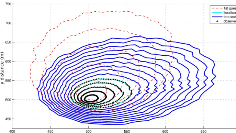
Figure 8. Five assimilated fire fronts with 1 min intervals (black solid lines). The first guess (red dashed line) is taken to be far from the
true invariants vector to check the algorithm capability to converge. A 10 min forecast (blue solid lines) is also calculated using fuel depth as sensor data.
required convergence which slightly increases the computing time.
Besides considering observed values for wind speed and direction, the forecast algorithm can also consider meteoro-logical predictions to deliver a more accurate forecast when these quantities vary. To illustrate this, five fire fronts are as-similated during 25 min (at a frequency of 1 fire front every 5 min). The invariants are perfectly identified with six itera-tions as shown in Fig. 7. Then, a forecast is launched for the next 25 min with a synthetic prediction of wind speed and direction.
3.5.2 Fuel depth as sensor data
We consider now the case where fuel depth is available and varies spatially but is constant. To cast the new invariants we use the information obtained with a sensitivity analysis per-formed on Rothermel’s model. The analysis reveals that RoS is linearly related to fuel depth δ as a first approximation. Thus, the RoS can now be written as
RoS=Imfw·δ(x, y), (23)
where fuel depthδ(x, y)varies spatially.
The wind contribution is now included in RoS=Imfwand therefore we have to create a new parameter that accounts for the shape of the elliptical firelets (i.e. the eccentricity):ILB, where LB stands for length-to-breadth ratio. This invariant also depends on wind speed and, thus, is not independent ofImfw. This does not affect the capacity of our forecasting model sinceILBcould be interpreted as a shaping factor and the way it is used in the forward model (only in the Huygens
expansion part) prevents it from being mixed withImfw. As in the previous cases the wind direction invariantIθ is required to close the invariant cast.
The effect of assimilating a space-dependent variable is that RoS now also depends on the location. This adds an ex-tra non-linear behaviour to the model, since now when the fire front location changes, the RoS changes as well. Despite this higher complexity, our algorithm handles it in the opti-misation loop and correctly matches the observations (Fig. 8) and identifies the invariants (Fig. 9).
3.6 Lead time
The lead time for the different implementations discussed above is investigated by assimilating different number of fire fronts and recording the computing time to deliver a 30 min forecast. The total assimilating time since it depends on the assimilation frequency (i.e. the number of assimilations per unit of time). Changing this frequency has a minor influence on the computing time since its contribution is linear in our forward model but might be important if more complex for-ward models (such as Computational Fluid Mechanics based, for example). The Rothermel variables that generate the syn-thetic data and the educated guess were kept constant for all the scenarios when they were not sensor data (such as wind speed, wind direction or fuel depth).
1st guest 1 2 3 −100
−50 0 50 100 150 200 250 300
off−set true vlaue [%]
# Iterations
1st guest 1 2 3 0
1 2 x 10⁴
Cost Function Value [m
2]
I
u Iθ Imfw Cost
Figure 9. Cost function and invariant convergence when fuel depth
is sensor data.
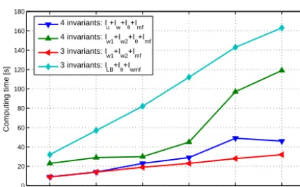
4 8 12 16 20 24
0 20 40 60 80 100 120 140 160 180
Number of assimilated fire fronts
Computing time [s]
4 invariants: Iu+Iw+Iθ+Imf 4 invariants: I
w1+Iw2+Iθ+Imf
3 invariants: I
w1+Iw2+Imf
3 invariants: ILB+Iθ+Iwmf
Figure 10. Computing time for all the implementations of the
fore-casting algorithm studied.
dimension of the matrices involved in the optimisation pro-cess decreases. The exception is when fuel information is data. The spatial dependency of the fuel depth and the fact that RoS has to be recalculated in every node raises the com-puting time, and thus this case is the slower one. The effect of feeding the algorithm with wind speed data becomes notice-able above 16 assimilated fronts when the complexity of the fire front shapes increases the number of iterations required to reach convergence.
Despite these significant differences, when eight fronts are assimilated the forecast is delivered in less than 1 min and even when 24 fronts are assimilated the lead time is well above 25 min for a 30 min forecast.
A laptop with dual processor core of 2.2 GHz is used as a computational tool since (as stated in the initial require-ments) the forecasting algorithm must be suitable for desktop computers.
1st guest 1 2 3
−100 −50 0 50 100 150 200
off−set true vlaue [%]
# Iterations
1st guest 1 2 3 0
5 x 10⁴
Cost Function Value [m
2]
I
LB Iθ Imfw Cost
Figure 11. Convergence of cost function (black dashed line) and
invariants (solid lines) when perturbed data are assimilated.
3.7 Effect of errors in the data
The fact that the synthetic data are generated with a Rothermel–Huygens model implies that there exists at least one true invariant vector that exactly generates the observed fronts. However, this is not the case in reality since the for-ward model used is only an approximation of the real fire dynamics. Thus, to test the forecasting algorithm in a situa-tion where such a true vector no longer exists (thus, perfect convergence is then impossible), the synthetic data used in the fuel depth sensor data case (Sect. 3.5.2) have been ran-domly perturbed with an error uniformly distributed in the range of[0±10]m. Apart from exploring the response of the forecasting algorithm in a case where the forward model can-not properly describe the fire locations, this test can be seen as a sensitivity check of the errors and accuracy involved in data acquisition.
As expected, the best optimisation does not match the ob-servations perfectly and, thus, the cost function converges to a value of 2500 m2instead of zero (see Fig. 11). Despite this fact, the convergence of the invariants – towards true values – is still reached with an error lower than 5 %.
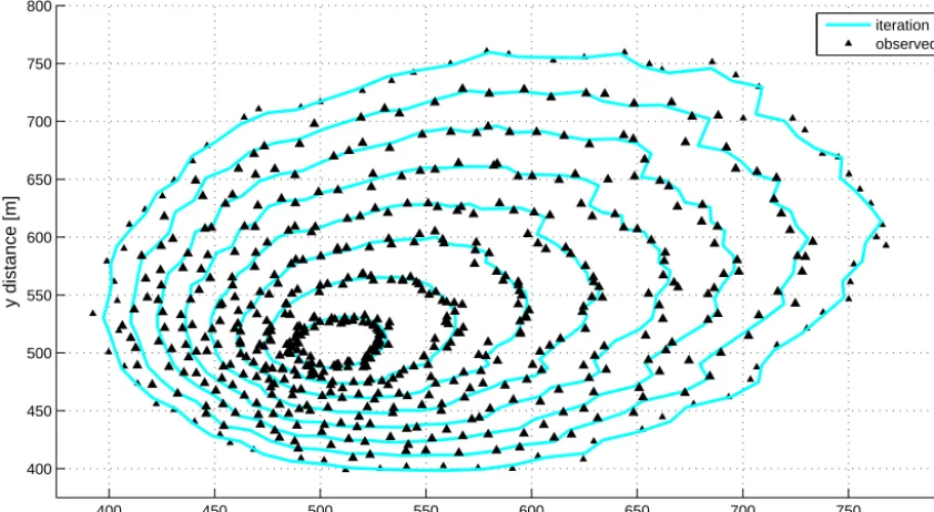
Figure 12 shows the observed fronts and the correspond-ing optimisation after four iterations. The sharp corners in the observed perimeters are due to the random distribution of the fuel depth and the added error. More tests performed while extending the error added to observation demonstrate that the algorithm manages to assimilate the observations with perturbations of up to±20 m in magnitude. The invariants also converged in this case which demonstrates the potential of this forecasting algorithm even when inaccurate data are available.
4 Conclusions
400 450 500 550 600 650 700 750 800 400
450 500 550 600 650 700 750 800
x distance [m]
y distance [m]
iteration 4 observed
Figure 12. Perturbed fire fronts (black lines) correctly assimilated after four integrations. The invariant cast used is this of Sect. 3.5.2 where
fuel depth is used as an input and three invariants are identified.
explored focusing on wind-driven wildfires. The algorithm framework is general enough to be valid to different sensor data or forward models. In this work the forward model is composed by use of Rothermel’s spread theory and Huy-gens expansion and is challenged with synthetically gener-ated front locations. The forecasting algorithm uses direct automatic differentiation and a tangent linearisation of the forward model to solve the optimisation problem. This strat-egy showed great efficiency finding the invariants within less than 10 iterations (runs of TLM), although special attention must be taken regarding multiplicity in the determination of the invariants. Multiplicity can be avoided by extending the forward model so that it predicts extra parameters (such as flame height or heat release rate) and assimilates them, or including extra information about the system to break the multiplicity. The latter was implemented and illustrated in two different scenarios. All the invariants were then correctly identified, even when the first guess greatly differed from the true value. All the implementations had a positive lead time (time ahead of the event). The most computationally expen-sive implementation is the one that uses fuel depth since the RoS varies in each node of the front.
Future work should study real sensor data (e.g. Coen et al., 2013) and look into improved (more accurate yet faster) models. To keep developing the methodology some identi-fied limitations should be tackled as spotting fires – which do not follow the classical (i.e. Rothermel) fire spread – and the capacity of the forecasting algorithm to deal with uncer-tainties caused by the lack of reliable data, and deliver prob-abilistic values as outputs. To pursue this, we propose to
in-crease the number of invariants to several dozen. Then the automatic direct differentiation should be switched to adjoint differentiation (adjoint modelling approach) to keep the low computational cost requirement.
A discussion on whether data assimilation should involve more complex models or not might be spurious at this point. This will be decided by the International wildfire commu-nity at large, specially the Fire Service. If the development of weather forecasting systems over the last few decades can serve as guidance somehow for wildfire forecasting systems, we note that they currently simulate weather patterns in a series of models of diverse complexity of which the grids range from fine and regional to global and coarse. So far, we can show that our wildfire forecast method is light, fast and flexible. It can be adapted to run on models of any complex-ity, and we show its strengths here using synthetic data and a model that, albeit rather simple, is the most widely used model by the international wildfire community.
Acknowledgements. Support for O. Rios from the Erasmus Mundus European Project and the International Master of Science in Fire Safety Engineering (IMFSE) is gratefully acknowledged. The authors also want to thank Elsa Pastor for comments that improved draft versions.
Edited by: D. Veynante
References
Anderson, H. E.: Predicting wind-driven wild land fire size and shape, US Department of Agriculture, Forest Service, Inter-mountain Forest and Range Experiment Station, 1983.
Coen, J. and Schroeder, W.: Use of spatially refined satellite re-mote sensing fire detection data to initialize and evaluate coupled weather-wildfire growth model simulations, Geophys. Res. Lett., 40, 5536–5541, 2013.
Cowlard, A., Jahn, W., Abecassis-Empis, C., Rein, G., and Torero, J. L.: Sensor assisted fire fighting, Fire Technol., 46, 719– 741, 2010.
Finney, M.: FARSITE, fire area simulator – model development and evaluation, vol. 3, US Department of Agriculture, Forest Service, Rocky Mountain Research Station, 1998.
Griewank, A.: Evaluating Derivatives: Principles and Techniques of Algorithmic Differentiation, no. 19 in Frontiers in Appl. Math., SIAM, Philadelphia, PA, 2000.
Jahn, W., Rein, G., and Torero, J. L.: Forecasting fire growth using an inverse zone modelling approach, Fire Safety J., 46, 81–88, 2011.
Jahn, W., Rein, G., and Torero, J. L.: Forecasting fire dynamics us-ing inverse computational fluid dynamics and tangent linearisa-tion, Adv. Eng. Softw., 47, 114–126, 2012.
Lautenberger, C.: Wildland fire modeling with an Eulerian level set method and automated calibration,. Fire Safety J., 62, 289– 298,2013.
Mandel, J., Bennethum, L. S., Beezley, J. D., Coen, J. L., Dou-glas, C. C., Kim, M., and Vodacek, A.: A wildland fire model with data assimilation, Math. Comput. Simulat., 79, 584–606, 2008.
Mandel, J., Beezley, J. D., Coen, J. L., and Kim, M.: Data assimila-tion for wildland fires, IEEE Contr. Syst. Mag., 29, 47–65, 2009.
Mutlu, M., Popescu, S. C., Stripling, C., and Spencer, T.: Mapping surface fuel models using lidar and multispectral data fusion for fire behavior, Remote Sens. Environ., 112, 274–285, 2008. Nocedal, J. and Wright, S. J.: Numerical Optimization, Springer
Se-ries in Operations Research and Financial Engineering, Springer, New York, 1999.
Richards, G. D.: An elliptical growth model of forest fire fronts and its numerical solution, Int. J. Numer. Meth. Eng., 30, 1163–1179, 1990.
Richards, G. D.: The properties of elliptical wildfire growth for time dependent fuel and meteorological conditions, Combust. Sci. Technol., 95, 357–383, 1993.
Rochoux, M. C., Delmotte, B., Cuenot, B., Ricci, S., and Trouvé, A.: Regional-scale simulations of wildland fire spread informed by real-time flame front observations, P. Combust. Inst., 34, 2641–2647, 2013.
Rochoux, M. C., Emery, C., Ricci, S., Cuenot, B., and Trouvé, A.: Towards predictive simulation of wildfire spread at regional scale, IAFSS 11th Symposium, 2014.
Rossi, L., Molinier, T., Akhloufi, M., Pieri, A., and Tison, Y.: Ad-vanced stereovision system for fire spreading study, Fire Safety J., 60, 64–72, 2013.
Rothermel, R.: A mathematical model for predicting fire spread in wildland fuels, Intermountain Forest & Range Experiment Sta-tion, Forest Service, US Department of Agriculture, 1972. Scott, J. and Burgan, R.: Standard fire behavior fuel models :
a comprehensive set for use with Rothermel’s surface fire spread model, USDA Forest Service, Rocky Mountain Research Station, General Technical Report RMRS-GTR-153, 72 pp., 2005. Sullivan, A. L.: Wildland surface fire spread modelling, 1990–2007.