Vol 10, No 7 (2019)

(1)

Available online through

ISSN 2229 – 5046

International Journal of Mathematical Archive- 10(7), July-2019 53

NEW RIDGE ESTIMATORS

OF SUR MODEL WHEN THE ERRORS ARE SERIALLY CORRELATED

MOHAMED REDA ABONAZEL*

Department of Applied Statistics and Econometrics,

Faculty of Graduate Studies for Statistical Research, Cairo University, Giza, Egypt.

(Received On: 11-07-19; Revised & Accepted On: 25-07-19)

ABSTRACT

T

his paper considers the seemingly unrelated regressions (SUR) model when the errors are first-order serially correlated as well as the explanatory variables are highly correlated. We proposed new ridge estimators for this model under these conditions. Moreover, the performance of the classical (Zellner’s and Parks’) estimators and the proposed (ridge) estimators has been examined by a Monte Carlo simulation study. The results indicated that the proposed estimators are efficient and reliable than the classical estimators.

Keywords: Biased estimators; GLS estimation method; Multicollinearity; Parks’ SUR model; Seemingly unrelated regressions model; Zellner’s SUR model.

1. INTRODUCTION

The SUR model has been proposed by Zellner (1962) under the assumption that the errors of the model are related by contemporaneous correlation. Then, Parks (1967) developed this model by assume that the errors are related by both serial and contemporaneous correlation. But the two models assume that the explanatory variables in the model are independent. But this assumption is very hard in empirical work, because most empirical datasets contain the correlated explanatory variables. This problem defined in econometrics literature with the multicollinearity problem. This problem arises in situations when the explanatory variables are highly inter-correlated. Then it becomes difficult to disentangle the separate effects of each of the explanatory variables on the dependent variable. As a result, the estimated coefficients may be statistically insignificant and/or have, unexpectedly, different signs. Thus, conducting a meaningful statistical inference would be difficult for the researcher.

To solve the multicollinearity problem in Zellner’s SUR model, Srivastava and Giles (1987) proposed the general ridge estimator for this model.0F

1_{Also several ridge estimators are proposed and compared by Alkhamisi and Shukur (2008)}

and Rana and Al Amin (2015). However, these papers not provided any solution of the multicollinearity problem for the SUR model under Parks’ assumption. Therefore, in this paper, we develop the ridge estimators for Parks’ SUR model.

This paper is organized as follows. Section 2 presents a background about Parks’ SUR model. The proposed ridge estimators of this model are provided in Section 3. While in Section 4, a simulation study is conducted to investigate the performance of the proposed estimators. Finally, Section 5 offers the concluding remarks.

Corresponding Author: Mohamed Reda Abonazel*

Department of Applied Statistics and Econometrics,

Faculty of Graduate Studies for Statistical Research, Cairo University, Giza, Egypt.

1_{In general, the ridge estimator was first proposed by Hoerl and Kennard (1970a,b), and later followed by many}

(2)

2. PARKS’ SUR MODEL

Consider the following SUR model, with 𝑚 regression equations:

𝑌

𝑚𝑛× 1 =𝑚𝑛𝑋×𝐾 𝐾𝐵× 1 +𝑚𝑛𝑈× 1 (1)

where 𝑌= (𝑦₁′, … ,𝑦_𝑚′)′is the vector of endogenous variable, and 𝑋=𝑑𝑖𝑎𝑔[𝑋_𝑖]; with 𝑋_𝑖 (for𝑖= 1, … ,𝑚) is the matrix of the exogenous variables of equation number 𝑖 with dimension𝑛×𝑘_𝑖, and 𝐵is the vector of the parameters with

𝐾 =∑𝑚𝑖=1𝑘𝑖, while 𝑈= (𝑢1′, … ,𝑢𝑚′ )′ is the errors vector.

Assumptions:

A1:𝑢_𝑖=𝜌_𝑖𝑢_𝑖,−1+𝜀_𝑖 for all 𝑖= 1, … ,𝑚, whrere 𝑢_𝑖,−1 is the first lag vector of 𝑢_𝑖, and 𝜌_𝑖 is the first-order serial correlation coefficient; where −1 <𝜌_𝑖< 1.

A2:𝐸(𝑢₁′, … ,𝑢_𝑚′ )′=𝐸(𝑈) = 0, 𝐸(𝜀₁′, … ,𝜀_𝑚′)′=𝐸(𝜀) = 0, and 𝐶𝑜𝑣(𝑈,𝜀) = 0

A3: 𝐶𝑜𝑣(𝑈) =𝐸(𝑈𝑈′) =�

𝜎11𝑉1 𝜎12𝐼𝑛 ⋯ 𝜎1𝑚𝐼𝑛

𝜎21𝐼𝑛 𝜎22𝑉2 ⋯ 𝜎2𝑚𝐼𝑛

⋮ ⋮ ⋱ ⋮

𝜎𝑚1𝐼𝑛 𝜎𝑚2𝐼𝑛 ⋯ 𝜎𝑚𝑚𝑉𝑚

�=Ω;

where 𝑉_𝑖= 1

1−𝜌_𝑖2

⎝ ⎛

1 𝜌𝑖 𝜌𝑖2 ⋯ 𝜌𝑖𝑛−1

𝜌𝑖 1 𝜌𝑖 ⋯ 𝜌𝑖𝑛−2

⋮ ⋮ ⋮ ⋱ ⋮

𝜌𝑖𝑛−1 𝜌𝑖𝑛−2 𝜌𝑖𝑛−3 ⋯ 1 ⎠

⎞_.

A4:𝑋 is non-stochastic matrix, 𝑐𝑜𝑣(𝑋,𝜀) = 0, and 𝑐𝑜𝑣(𝑋,𝑈) = 0.

A5:𝑋 is full column rank matrix, i.e., 𝑟𝑎𝑛𝑘(𝑋) =𝐾.

Under these assumptions, we can apply the generalized least squares (GLS) method on equation (1) to estimate 𝐵:

𝐵�𝑃= (𝑋′Ω−1𝑋)−1𝑋′Ω−1𝑌, and 𝑀𝑆𝐸�𝐵�𝑃�= (𝑋′Ω−1𝑋)−1.

The model above with these assumptions is discussed by Parks (1967). But if 𝑉_𝑖=𝐼_𝑛, we will back to Zellner’s SUR model, and then Zellner’s estimator is

𝐵�𝑍 = [𝑋′(Σ−1⨂𝐼𝑛)𝑋]−1𝑋′(Σ−1⨂𝐼𝑛)𝑌,and 𝑀𝑆𝐸�𝐵�𝑍�= [𝑋′(Σ−1⨂𝐼𝑛)𝑋]−1, (2)

where Σ=�

𝜎11 𝜎12 ⋯ 𝜎1𝑚

𝜎21 𝜎22 ⋯ 𝜎2𝑚

⋮ ⋮ ⋱ ⋮

𝜎𝑚1 𝜎𝑚2 ⋯ 𝜎𝑚𝑚

�.

3. PROPOSED RIDGE ESTIMATORS

In this paper, we develop the ridge estimation of the Parks’ model, to solve the multicollinearity problem. The ridge estimator of this model and MSE of it are given by:

𝐵�𝑅𝑃= (𝑋′Ω−1𝑋+𝑅)−1𝑋′Ω−1𝑌;

𝑀𝑆𝐸�𝐵�𝑅𝑃�= (𝑋′Ω−1𝑋+𝑅)−1(𝑋′Ω−1𝑋+𝑅𝐵𝐵′𝑅′)(𝑋′Ω−1𝑋+𝑅)−1, (3)

where 𝑅 is a 𝐾×𝐾 matrix with nonnegative elements:

𝑅=�

𝑅1 0 ⋯ 0

0 𝑅2 ⋯ 0

⋮ ⋮ ⋱ ⋮

0 0 ⋯ 𝑅𝑚

�; with 𝑅_𝑖= 𝑑𝑖𝑎𝑔�𝑟_𝑖1, … ,𝑟_𝑖𝑘_𝑖�∀𝑖= 1, … ,𝑚.

The canonical version of model (1) is given by:

𝑌∗₌_𝑍𝛼₊_𝑈∗_,

(4)

where 𝑌∗=Ω−1/2𝑌 , 𝑈∗=Ω−1/2𝑈 , 𝑍=𝑋∗Φ with 𝑋∗=Ω−1/2𝑋 and Φ eigenvectors of (𝑋∗′𝑋∗) , then

𝑍′_𝑍₌_Φ′_𝑋∗′_𝑋∗_Φ₌_Λ_{, where}_Λ_{the eigenvalues of}₍_𝑋∗′_𝑋∗₎_{. The corresponding GLS estimator of (4) is}

𝛼� = (𝑍′_𝑍₎−1_𝑍′_𝑌∗_{. Srivastava and Giles (1987) and Firinguetti (1997) proved that the optimum elements of}_𝑅_are

𝑟̂𝑖𝑗 =_𝛼�1 𝑖𝑗

2 ; 𝑖= 1, … ,𝑚;𝑗= 1, … ,𝑘𝑖, if and only if the following conditions are holds: 𝛼′Λ𝛼< 1 and 𝛼′𝑅𝛼< 2. Note

(3)

In this paper, we propose new ridge estimators of this model basing on the following ridge parameters:

1- The median of 𝑟_𝑖𝑗 that proposed by Kibria (2003) for single equation version and Alkhamisi and Shukur (2008) developed it for SUR model:

𝑟̂𝑖𝑗(𝑆𝐾) =𝑚𝑒𝑑𝑖𝑎𝑛 �_𝛼�1

𝑖𝑗2�.

2- The max of 𝑟_𝑖𝑗 that proposed by Alkhamisi and Shukur (2008):

𝑟̂𝑖𝑗(𝐴𝑆) =𝑚𝑎𝑥 �_𝛼�1 𝑖𝑗 2�.

3- Let 𝐾�=𝐾/𝑚, we suggest using the following ridge parameters:

𝑟̂𝑖𝑗(𝑛𝑒𝑤1) =�𝑟̂𝑖𝑗(𝑆𝐾)�1/𝐾��𝑟̂𝑖𝑗(𝐴𝑆)�1/𝐾�;

𝑟̂𝑖𝑗(𝑛𝑒𝑤2) =�𝑠𝑢𝑚 �_𝛼�1

𝑖𝑗2�� 1/𝐾�

�𝑟̂𝑖𝑗(𝐴𝑆)�1/𝐾�.

Since 𝐵�_𝑅 estimator still involves the unknown parameters, therefore it needs to estimate these parameters to make this estimator feasible. We suggest using the following consistent estimators:2

𝜌�𝑖=∑ 𝑢�𝑖𝑡𝑢�𝑖,𝑡−1 𝑛

𝑡=2

∑𝑛𝑡=2𝑢�_𝑖2_,_𝑡−1 , and 𝜎�𝑖𝑠=

𝜀�_𝑖′𝜀�𝑠

(𝑛−𝑘_𝑖)1/2_{(𝑛−𝑘𝑠}₎1/2 ∀𝑖=𝑠= 1, … ,𝑚,

where 𝑢�_𝑖= (𝑢�_𝑖1, … ,𝑢�_𝑖𝑛)′ is the residuals vector obtained from applying OLS on equation number 𝑖 ,

𝜀̂𝑖= (𝜀̂𝑖1, … ,𝜀̂𝑖𝑛)′; 𝜀̂𝑖1=𝑢�𝑖1�1− 𝜌�𝑖2 , and 𝜀̂𝑖𝑡=𝑢�𝑖𝑡− 𝜌�𝑖𝑢�𝑖,𝑡−1 for 𝑡= 2, … ,𝑛.

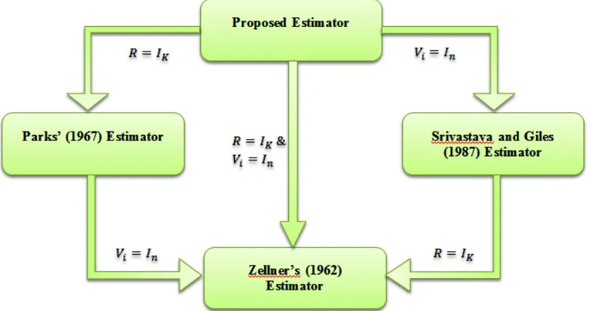
Figure-1: The transformations from the proposed estimator to other estimator

Figure 1 shows that the proposed estimator is a general estimator of three estimators (Srivastava and Giles (1987), Parks’, and Zellner’s estimators). In other words, we can say that these estimators are special cases of the proposed estimator.

4. MONTE CARLO SIMULATION STUDY

In this section, we conduct a comparative study between the classical (Parks’ and Zellner’s) estimators and the four ridge estimators (SK, AS, new1, and new2) through the Monte Carlo simulation study. In our simulation study, Monte Carlo experiments were performed based on the model in (1). To investigate the performance of these estimators in different situations, we will use different simulation factors as show in Table 1. R software is used to perform this study.3

2_{The properties of these estimators are studied by Parks (1967).}

(4)

To judge the performance of six estimators, the total mean squared error (TMSE) criterion is used:

TMSE�𝛽̂�= 1_𝐿∑𝐿𝑙=1(𝛽̂𝑙− 𝛽)′(𝛽̂𝑙− 𝛽),

where 𝛽̂_𝑙 is the vector of estimated values at 𝑙𝑡ℎ experiment of 𝐿= 1000 Monte Carlo experiments, while 𝛽is the vector of true coefficients.

Table-1: The simulation factors of our study

Simulation factor Levels The number of parameters (𝑩) in each equation (without

intercept) 𝑘_𝑖= 4 or 6

The number of equations (𝒎) 𝑚 = 2, 4, or 6 The true values of 𝑩 (as Månsson and Shukur, 2011 and

KaÇiranlar and Dawoud, 2018)

𝐵′𝐵= 1 and

𝛽1=⋯=𝛽𝑚

The sample size in each equation (𝒏)

𝑛 = 25, 50, 75, or 100 The explanatory variables: 𝑿~𝑴𝑽𝑵(𝟏,𝜮_𝑿), where diag

(𝚺_𝒙) = 1 and off-diag (𝚺_𝒙) = 𝝆_𝒙 (as Alkhamisi and

Shukur, 2008 and Abonazel and Farghali, 2018) 𝜌_𝑥= .90, .95, or .99 The error term: 𝑼~𝑴𝑽𝑵(𝟎,𝛀), where 𝝈_𝒊𝒊=𝟏, 𝝈_𝒊𝒔=

.𝟖𝟎∀𝒊 ≠ 𝒔; 𝒊=𝒔=𝟏, … ,𝒎, and 𝝆_𝒊 is 𝜌_𝑖=𝜌=.75 or .90

The results are given in Tables 2-7. Specifically, Tables 2, 4, and 6 present the TMSE values of the estimators when

𝑘𝑖= 4, while case of 𝑘𝑖= 6 is presented in Tables 3, 5, and 7. From Tables 2-7, we can summarize some effects for all

estimators in the following points:

• If the value of 𝑛is increased, the values of TMSE are decreasing for all simulation situations.

• If the values of 𝑚and𝜌 are increased, the values of TMSE are increasing in all situations.

However, if the values of 𝑘_𝑖, 𝜌_𝑥, and 𝜌 are increased, the TMSE values of Parks’ and Zellner’s estimators are increased more than ridge estimators. In other words, the ridge estimators are efficient than Parks’ and Zellner’s estimators. Specifically, the new2 estimator is the best estimator because it has minimum TMSE in all simulation situations.

5. CONCLUSION

In this paper, we developed new ridge estimators for SUR model when there are high inter-correlations between the explanatory variables as well as the errors are serially correlated. A Monte Carlo simulation study was conducted to evaluate the performance of the classical estimators and different ridge estimators. The simulation results indicated that the ridge estimators are efficient than classical estimators in all situations. Moreover, the ridge estimators which based on the proposed parameters 𝑟̂_𝑖𝑗(𝑛𝑒𝑤1) and𝑟̂_𝑖𝑗(𝑛𝑒𝑤2) are more efficient than other ridge estimators. And the new2 estimator is the best ridge estimator for this model.

Table-2: TMSE values for the different estimators when 𝑚= 2 and 𝑘_𝑖= 4

𝒏 GLS estimators Ridge estimators

Zellner Parks SK AS new1 new2

𝝆=.𝟕𝟓,𝝆𝒙=.𝟗𝟎

25 3.3093 2.8132 0.5662 0.4290 0.4107 0.2434 50 1.9638 0.8717 0.1898 0.4322 0.1995 0.1365 75 1.4756 0.8921 0.2873 0.4425 0.2978 0.2187 100 0.7433 0.5846 0.1850 0.4023 0.2111 0.1444

𝝆=.𝟕𝟓,𝝆𝒙=.𝟗𝟓

25 10.5349 6.8406 0.6441 0.3898 0.3819 0.2005 50 3.2643 2.4891 0.4964 0.3292 0.3774 0.1977 75 1.9457 1.5986 0.3309 0.3485 0.2808 0.1617 100 1.7389 1.0083 0.2293 0.3833 0.2359 0.1537

𝝆=.𝟕𝟓,𝝆𝒙=.𝟗𝟗

25 64.5727 29.0269 1.1529 0.2699 0.3252 0.1682 50 14.9609 15.3605 1.5979 0.2907 0.4549 0.1938 75 10.6514 6.8152 0.7066 0.2744 0.3761 0.2069 100 5.4922 4.0121 0.5068 0.2736 0.2491 0.1095

𝝆=.𝟗𝟎,𝝆𝒙=.𝟗𝟎

(5)

100 1.6578 1.0216 0.2294 0.4804 0.2302 0.1695

𝝆=.𝟗𝟎,𝝆𝒙=.𝟗𝟓

25 17.3703 13.4405 1.3889 0.4474 0.5614 0.3325 50 7.2449 3.5487 0.4274 0.4183 0.2965 0.1898 75 4.7687 2.1814 0.3775 0.4086 0.2872 0.1822 100 6.4977 1.7847 0.3213 0.3787 0.2833 0.1820

𝝆=.𝟗𝟎,𝝆𝒙=.𝟗𝟗

25 76.2155 40.0421 2.2786 0.3703 0.5024 0.2536 50 35.1001 15.7828 0.8277 0.2770 0.3008 0.1646 75 24.9208 20.3456 2.1830 0.3659 0.6939 0.3422 100 37.7388 7.9543 0.6389 0.2339 0.2798 0.1299

𝝆=.𝟕𝟓,𝝆𝒙=.𝟗𝟎

25 6.0869 4.9353 0.4805 0.4744 0.5549 0.2602 50 2.1677 1.6487 0.2374 0.4843 0.4070 0.2136 75 2.1376 1.6900 0.3605 0.4338 0.5612 0.3078 100 1.1635 0.8936 0.1945 0.4622 0.3883 0.2320

𝝆=.𝟕𝟓,𝝆𝒙=.𝟗𝟓

25 18.8283 10.7105 1.4818 0.3611 1.0309 0.4630 50 8.0270 5.0371 0.6325 0.3790 0.6987 0.3335 75 3.9324 2.9416 0.5416 0.3878 0.6590 0.3314 100 2.8857 1.5957 0.2380 0.4277 0.4339 0.2247

𝝆=.𝟕𝟓,𝝆𝒙=.𝟗𝟗

25 80.0961 50.8054 4.8144 0.3225 1.0006 0.4121 50 23.0518 21.7883 1.9871 0.2899 0.7741 0.3087 75 33.2683 12.1523 1.0189 0.2484 0.6152 0.2440 100 16.0482 7.0348 0.6724 0.2693 0.5094 0.1950

𝝆=.𝟗𝟎,𝝆𝒙=.𝟗𝟎

25 22.7738 17.0336 2.4325 0.5397 1.3022 0.6262 50 10.0682 6.0696 0.7376 0.5305 0.7956 0.3895 75 6.2711 3.0931 0.5817 0.5007 0.7453 0.4126 100 3.2779 1.3125 0.1958 0.5475 0.3745 0.2122

𝝆=.𝟗𝟎,𝝆𝒙=.𝟗𝟓

25 26.8653 22.1972 1.2221 0.4851 0.6291 0.2887 50 12.8952 6.6694 0.6216 0.4551 0.5674 0.2573 75 9.9596 9.5709 1.6845 0.3875 1.2132 0.5635 100 6.1629 3.0764 0.3267 0.4544 0.4918 0.2307

𝝆=.𝟗𝟎,𝝆𝒙=.𝟗𝟗

(6)

𝝆=.𝟕𝟓,𝝆𝒙=.𝟗𝟎

25 7.0932 5.4229 0.6376 0.6180 0.4221 0.2427 50 2.7313 1.8013 0.2767 0.6812 0.2699 0.1900 75 2.4684 1.6725 0.3218 0.6406 0.3099 0.1996 100 1.3302 0.6680 0.0903 0.7315 0.1246 0.1242

𝝆=.𝟕𝟓,𝝆𝒙=.𝟗𝟓

25 20.7810 15.8471 1.3541 0.5581 0.5878 0.2783 50 5.5935 3.6247 0.4217 0.5929 0.3089 0.1707 75 6.6071 4.7564 0.6663 0.5255 0.4559 0.2136 100 2.1297 1.2059 0.1279 0.6167 0.1536 0.1091

𝝆=.𝟕𝟓,𝝆𝒙=.𝟗𝟗

25 113.6974 95.0786 7.8941 0.4621 0.8608 0.3342 50 25.9463 16.9079 0.7986 0.4420 0.2752 0.1318 75 27.6831 16.4686 0.9874 0.3851 0.3463 0.1339 100 9.3053 5.5652 0.3359 0.5057 0.1669 0.0846

𝝆=.𝟗𝟎,𝝆𝒙=.𝟗𝟎

25 15.8385 11.3784 1.3109 0.6949 0.7106 0.4109 50 6.2572 2.9468 0.3763 0.7426 0.3202 0.2751 75 7.1595 2.7141 0.4380 0.6666 0.3467 0.2228 100 3.4778 1.2267 0.1622 0.7427 0.1786 0.1834

𝝆=.𝟗𝟎,𝝆𝒙=.𝟗𝟓

25 42.7804 23.5079 1.8264 0.6190 0.6827 0.3665 50 11.3087 5.6150 0.5294 0.6180 0.3570 0.2307 75 11.3110 5.6140 0.7155 0.6171 0.4577 0.2646 100 5.2760 2.1381 0.2182 0.6520 0.1989 0.1549

𝝆=.𝟗𝟎,𝝆𝒙=.𝟗𝟗

(7)

𝝆=.𝟕𝟓,𝝆𝒙=.𝟗𝟎

25 16.8465 13.1986 1.0562 0.6676 0.9840 0.3417 50 4.6038 3.4177 0.3246 0.7259 0.6209 0.2279 75 3.7594 3.2273 0.4822 0.7142 0.7731 0.3087 100 1.7489 1.1432 0.1022 0.7779 0.3624 0.1579

𝝆=.𝟕𝟓,𝝆𝒙=.𝟗𝟓

25 36.5553 25.6178 2.2447 0.5874 1.2485 0.3990 50 10.8707 8.8997 0.8008 0.6222 0.8868 0.3196 75 7.4498 5.8000 0.6238 0.6173 0.8033 0.2815 100 3.5236 1.8671 0.1404 0.7208 0.4102 0.1541

𝝆=.𝟕𝟓,𝝆𝒙=.𝟗𝟗

25 169.7513 150.4132 9.8967 0.4188 1.1344 0.2985 50 55.0262 38.1009 1.5649 0.4687 0.6665 0.1833 75 38.6596 31.7640 2.5263 0.4106 1.0364 0.2811 100 17.5981 10.3540 0.5447 0.5344 0.5054 0.1225

𝝆=.𝟗𝟎,𝝆𝒙=.𝟗𝟎

25 41.9803 22.4930 1.9984 0.7424 1.2546 0.4909 50 11.2528 4.8031 0.4819 0.8075 0.6931 0.3232 75 6.7004 4.5999 0.5688 0.7442 0.7907 0.3618 100 4.1897 1.6760 0.1359 0.8086 0.3526 0.1524

𝝆=.𝟗𝟎,𝝆𝒙=.𝟗𝟓

25 67.5143 72.4064 5.5347 0.6184 1.6124 0.5655 50 19.8076 10.2837 0.6387 0.7189 0.6434 0.2393 75 15.8237 10.0435 1.0654 0.6136 0.9662 0.3661 100 8.2728 2.7418 0.1579 0.7359 0.3676 0.1346

𝝆=.𝟗𝟎,𝝆𝒙=.𝟗𝟗

(8)

𝝆=.𝟕𝟓,𝝆𝒙=.𝟗𝟎

25 13.1908 9.3313 0.9860 0.7433 0.5123 0.2598 50 4.1172 2.3364 0.2908 0.8153 0.2747 0.2332 75 2.4507 1.1278 0.1460 0.8166 0.1754 0.1759 100 1.9554 1.0619 0.1622 0.7737 0.1971 0.1535

𝝆=.𝟕𝟓,𝝆𝒙=.𝟗𝟓

25 41.2118 30.5880 3.2372 0.6794 0.8124 0.3095 50 8.1734 4.3377 0.3959 0.7029 0.2801 0.1620 75 4.8312 2.4020 0.2178 0.7478 0.2061 0.1556 100 4.1129 2.2568 0.2517 0.7152 0.2349 0.1464

𝝆=.𝟕𝟓,𝝆𝒙=.𝟗𝟗

25 127.5892 98.9370 5.3107 0.5734 0.6111 0.2635 50 41.3215 25.0368 0.9554 0.5450 0.2801 0.1258 75 22.1921 12.1928 0.5790 0.5915 0.2004 0.0887 100 16.7432 9.3874 0.5003 0.5712 0.2275 0.1115

𝝆=.𝟗𝟎,𝝆𝒙=.𝟗𝟎

25 37.9816 19.5995 1.5264 0.7903 0.7251 0.4153 50 10.5094 4.3923 0.4768 0.8169 0.3684 0.3001 75 6.0622 1.7671 0.1880 0.8502 0.1949 0.2428 100 5.3421 1.7021 0.2544 0.8174 0.2505 0.2270

𝝆=.𝟗𝟎,𝝆𝒙=.𝟗𝟓

25 54.0946 31.5410 2.3574 0.7735 0.8462 0.4899 50 17.1570 6.6839 0.4138 0.7620 0.2668 0.2371 75 15.9178 4.6703 0.3030 0.7567 0.2340 0.1910 100 11.4185 3.2598 0.3106 0.7554 0.2568 0.2030

𝝆=.𝟗𝟎,𝝆𝒙=.𝟗𝟗

(9)

𝝆=.𝟕𝟓,𝝆𝒙=.𝟗𝟎

25 23.5063 17.8416 1.2763 0.7880 1.2509 0.3610 50 8.2999 4.7767 0.4063 0.8438 0.7827 0.2695 75 4.4318 2.2069 0.1833 0.8652 0.5262 0.1872 100 3.9531 2.0619 0.2135 0.8251 0.5929 0.2216

𝝆=.𝟕𝟓,𝝆𝒙=.𝟗𝟓

25 64.7327 52.2059 4.1619 0.7294 1.8123 0.4940 50 17.4715 9.9942 0.7164 0.7382 0.9191 0.2613 75 7.4082 4.1413 0.2701 0.8049 0.6118 0.1781 100 7.8235 4.0963 0.3471 0.7642 0.7084 0.2102

𝝆=.𝟕𝟓,𝝆𝒙=.𝟗𝟗

25 330.3648 245.4258 11.0351 0.6163 1.1191 0.2919 50 80.5724 48.9693 2.2113 0.6169 0.8576 0.1929 75 40.1462 20.8563 0.8985 0.6257 0.6670 0.1408 100 38.7441 19.6973 1.1073 0.5804 0.8298 0.1753

𝝆=.𝟗𝟎,𝝆𝒙=.𝟗𝟎

25 56.9650 36.1794 3.3353 0.8242 1.9120 0.6542 50 21.8188 10.5090 0.7616 0.8405 0.9688 0.3395 75 10.9613 3.9171 0.2821 0.8793 0.5785 0.2293 100 9.2270 2.9419 0.2515 0.8748 0.5663 0.2257

𝝆=.𝟗𝟎,𝝆𝒙=.𝟗𝟓

25 117.9301 70.2598 3.6470 0.7898 1.3298 0.4357 50 39.7162 17.3205 0.7861 0.7818 0.7812 0.2409 75 17.7821 5.6742 0.2749 0.8510 0.5013 0.1763 100 15.9975 5.0113 0.2991 0.7953 0.5590 0.1758

𝝆=.𝟗𝟎,𝝆𝒙=.𝟗𝟗

25 535.6719 277.0767 14.1436 0.5895 1.1646 0.3146 50 271.4577 92.6541 2.5172 0.6084 0.6868 0.1785 75 93.6418 31.1750 0.8587 0.6557 0.5084 0.1284 100 68.2881 25.6952 0.9064 0.6249 0.6197 0.1820

REFERENCES

1. Abonazel, M. R. (2018). A practical guide for creating Monte Carlo simulation studies using R. International Journal of Mathematics and Computational Science, 4(1), 18–33.

2. Abonazel, M. R. and Farghali, R. A. (2018). Liu-type multinomial logistic estimator. Sankhya B: The Indian Journal of Statistics. https://doi.org/10.1007/s13571-018-0171-4.

3. Alkhamisi, M., Khalaf, G., Shukur, G. (2006). Some modifications for choosing ridge parameters. Communications in Statistics-Theory and Methods, 35(11): 2005-2020.

4. Alkhamisi, M., Shukur, G. (2008). Developing ridge parameters for SUR model. Communications in Statistics-Theory and Methods, 37(4): 544-564.

5. Firinguetti, L. (1997). Ridge regression in the context of a system of seemingly unrelated regression equations. Journal of Statistical Computation and Simulation, 56(2):145-162.

6. Hoerl, A. E., Kennard, R. W. (1970a). Ridge regression: Biased estimation for nonorthogonal problems. Technometrics, 12(1):55-67.

7. Hoerl, A. E., Kennard, R. W. (1970b). Ridge regression: applications to nonorthogonal problems. Technometrics, 12(1):69-82.

8. Kaçıranlar, S. and Dawoud, I. (2018). On the performance of the Poisson and the negative binomial ridge predictors. Communications in Statistics-Simulation and Computation, 47(6), 1751-1770.

9. Kibria, B. G. (2003). Performance of some new ridge regression estimators. Communications in Statistics-Simulation and Computation, 32(2):419-435.

10. Locking, H., Månsson, K., and Shukur, G. (2013). Performance of some ridge parameters for probit regression: with application to Swedish job search data. Communications in Statistics-Simulation and Computation, 42(3), 698-710.

(10)

12. Parks, R. W. (1967). Efficient estimation of a system of regression equations when disturbances are both

serially and contemporaneously correlated. Journal of the American Statistical Association, 62(318), 500-509.

13. Saleh, A. M. E., Kibria, B. M. G. (1993). Performance of some new preliminary test ridge regression estimators and their properties. Communications in Statistics-Theory and Methods, 22(10):2747-2764.

14. Rady, E. A., Abonazel, M. R., and Taha I. M. (2018). Ridge estimators for the negative binomial regression model with application. The 53rd Annual Conference on Statistics, Computer Science, and Operation Research 3-5 Dec, 2018. ISSR, Cairo University.

15. Rana, S., Al Amin, M. (2015). An alternative method of estimation of SUR model. American Journal of Theoretical and Applied Statistics, 4(3): 150-155.

16. Srivastava, V. K., Giles, D. E. (1987). Seemingly unrelated regression equations models: estimation and inference (Vol. 80). CRC Press.

17. Zellner, A. (1962). An efficient method of estimating seemingly unrelated regressions and tests for aggregation bias. Journal of the American statistical Association, 57(298):348-368.

Source of support: Nil, Conflict of interest: None Declared.