Exploring a Design Space of Schemes for
Detecting Programming Difficulty from
Interaction Logs
By Kun Wang
Senior Honors Thesis Computer Science
University of North Carolina at Chapel Hill
April 12, 2015
Approved:
______________________ Prasun Dewan, Thesis Advisor
1. Abstract
Detection of programming difficulty can be used effectively in various settings to promote
learning and instruction. This project extends existing work on programmer difficulty detection from
Eclipse and web logs by developing and evaluating a design space of difficulty detection schemes. Each
scheme in the design space consists of mapping from input vectors to a set of classifier attributes,
difficulty classifiers that make inferences based on these attributes, and sampling techniques to address
class imbalance. The schemes draw attributes from the following attribute set: edit, insertion, deletion,
focus, navigate, debug, and web access. They differ based on (a) mapping of input vectors to attribute set,
(b) difficulty classifiers, and (c) sampling techniques. The schemes are evaluated with 10 fold
cross-validation and leave-one-out participant model cross-validation techniques. Our analysis shows that different
schemes are appropriate for different applications of difficulty detection. Schemes with J48 decision tree
are the most capable of accurately prediction true negatives, not stuck, and should be employed in
real-time code collaboration to minimize false alarms and wasting the helper’s real-time. In comparison, schemes
with AdaBoost.M1 using Decision Stump as weak classifier have a high true positive accuracy, and
should instead be prioritized in API testing and difficulty stuck points studies as positive, stuck, points
often indicate major issues with design.
2. Introduction
Difficulty is defined as the perceived lack of progress while programming. It can originate from
many sources; some examples are syntax errors, semantics mistakes, and errors in tools and the libraries
we use. Difficulty prediction has immense utilitarian value. Detection and communication of difficulty
can allow for difficulty-based real-time collaboration; programmers with free time can elect to assist other
programmers encountering difficulty. Another general application of difficulty prediction is difficulty
stuck point analysis. The current research is part of a greater difficulty detection framework,
EclipseHelper. This system provides an implementation of stuck point analysis where the user can
detection can be applied to API design where different versions of an API can be field tested in difficulty
studies. It would be prudent to use the API implementation that results in the least amount of difficulty. In
education, difficulty detection can be used to gauge the difficulty of assignments and locate sections
where students consistently have difficulty; such indicators are effective in pinpointing materials needing
more elaboration and explanations.
Previous research by Carter in Automatic Difficulty Detection had achieved great results with difficulty prediction schemes A1J which he composed from A0J [1]. The current research explores a
larger design space of difficulty prediction schemes to construct improved schemes that has better stuck
class prediction and overall prediction accuracies.
Before we engage in further analysis, it is important to define a general model for difficulty
prediction schemes from which our design space arises. Section 3 outlines the general model and its
design dimensions. Section 4, 5, and 6 are the analysis sections. Section 4 analyzes the performance of
difficulty prediction schemes with tenfold cross-validation. Section 5 assesses the difficulty prediction
schemes under real-world circumstances with leave-one-out participant analysis. Section 6 evaluates the
effect of oversampling on the various schemes’ prediction accuracies. Section 7 concludes the paper and
introduces possible future works. Appendix A details the difference in attribute mappings. Appendix B
details the prediction tracker, a platform used to conduct much of the exploration done in this research.
3. Design Space of Difficulty Prediction Scheme
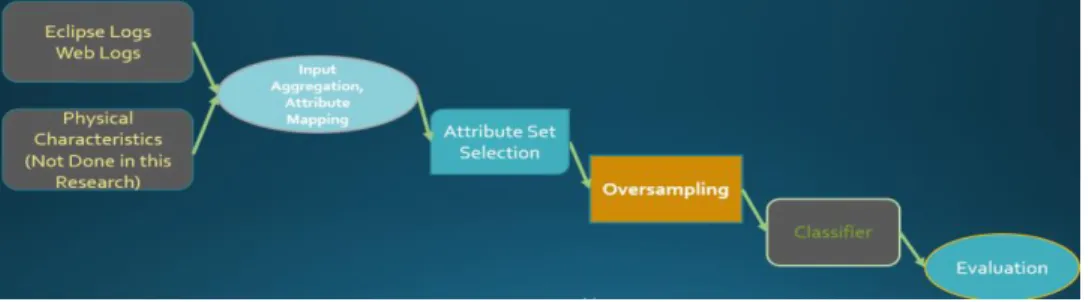
The general model for difficulty prediction is shown in figure 1.
The current research is the direct descendant of Carter’s research done in Automatic Difficulty Detection [1]. Carter conducted a user study to collect Eclipse events from 16 different participants but only used data from 10 participants; the current research uses all 16 participants’ data and adds in one
more participant. The Eclipse events and web activities from the participants form the Eclipse logs and
web logs, respectively. The two logs are the basis of the input dimension which is shared between all
schemes. Physical characteristics of the programmer is also another possible input method, but it is not
explored in the scope of this research due to being difficult to process and limited in use.
Additionally, Carter defined a base difficulty detection scheme in his research, A0J. Scheme A0J
is as follows:
Eclipse events are mapped with M0 mapping (discussed later) to classifier dataset attributes.
The attribute set for the classifier are edit, debug, navigation, and focus.
SMOTE is used to oversample the classifier dataset.
J48 decision tree is the classifier.
Cross-validation is the model validation technique.
The result of ten-fold cross validation analysis with A0J is shown in table 1. Due to low true positive
accuracy, Carter devised scheme A1J which split the edit attribute into insertion and deletion attributes.
Scheme A1J uses the M1 mapping (discussed later). A1J achieved much higher true positive accuracy,
72.7%, than A0J while maintaining high overall prediction accuracy.
Scheme A0J A1J
Overall Accuracy 770/814 (94.59%) 779/814 (95.70%)
True Negative 759/759 (100%) 739/759 (97.36%)
Table 1: Scheme A0J and A1J 10 Fold Cross-Validation Results
Since A1J is superior to A0J in true positive accuracy and slightly better in overall prediction
accuracy as seen in table 1, A1J served as the baseline for comparison with the newer schemes explored
in the current work. A0J is used in section 4, analysis, to only ascertain that the current research’s analysis
environment is consistent with Carter’s analysis environment.
The current research examines 4 different scheme families. Scheme families are examined instead
of individual schemes as presenting data from the vast number of possible schemes would pose a
challenge. A scheme family has fixed mapping and attribute set dimensions while classifier and
oversampling dimensions are dynamic so that we can fit better classifiers and oversampling techniques to
each mapping and attribute set combination. Scheme families A0 and A1 are devised with Carter’s
original A0J and A1J’s respective mapping and attribute set. A0 and A1 can give us a better measure of
A0J and A1J’s performances with all 17 participants’ data, and with different classifiers in the case of
A1J. Scheme family A2 is used to test the effectiveness of the additional classifier dataset attribute,
weblinks. Otherwise, A2 is identical to scheme family A1 [1]. Scheme family A3 uses its own mapping
for insertion and deletion attributes to analyze the difference between mappings while keeping other
dimensions constant. Please consult appendix A1-3 for more details on the actual java implementation of
the mappings.
A fundamental difference between Carter’s schemes and the schemes explored in this research is
input mapping. As mentioned earlier, Input mapping is the process of mapping input events from Eclipse
logs and web logs to classifier dataset attributes, the second dimension in the general model. Four
mappings are explored in this paper: M0, M1, M2, and M3. There are 7 different classifier attributes in
the attribute set dimension that each mapping selectively maps to: edit, insertion, deletion, navigation,
focus, weblinks, and debug. All four mapping maps to focus, debug, and navigation attributes in the same
maps anything edit related in Eclipse such as insert, redo, undo, and delete commands to the edit attribute.
M1 is from scheme A1J and scheme family A1 where the edit attribute was split into the insertion and
deletion attributes; therefore, M1 maps to the insertion and deletion attributes instead of the edit attribute.
M1’s insertion and deletion mappings are described in appendix A2. M2 is scheme family A2’s mapping;
it is an extension of M1 mapping to include mapping to the weblinks attribute. M3 maps to the same
attribute set as M2, but both map Eclipse events to the insertion and deletion attributes differently as
shown in Table 2. M3 maps cut and redo to the insertion attribute, but it does not map movecaret to the
insertion attribute; M2 maps movecaret to the insertion attribute but does not map cut and redo to the
insertion attribute. Furthermore, M3 maps undo to deletion and does not map cut to deletion while M2
does the opposite. M3’s insertion and deletion mappings are in appendix A3. After mapping to classifier
attributes, multiple Eclipse events are aggregated into a single segment. The segment serves as a classifier
dataset instance.
M2 M3
Insertion MoveCaret Cut
Redo
Deletion Cut Undo
Table 2: Different between M1/M2 and M3 Insertion and Deletion Mapping
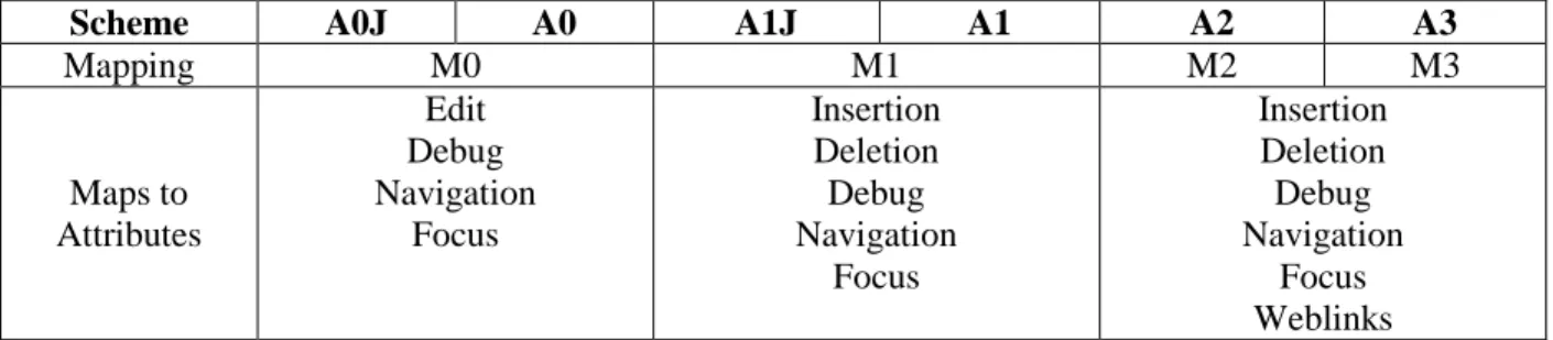
Table 3 summarizes the various schemes and scheme families, their respective mappings, and
their attribute sets.
Scheme A0J A0 A1J A1 A2 A3
Mapping M0 M1 M2 M3
Maps to Attributes Edit Debug Navigation Focus Insertion Deletion Debug Navigation Focus Insertion Deletion Debug Navigation Focus Weblinks
Table 3: Mapping Dimension of Schemes to Attributes
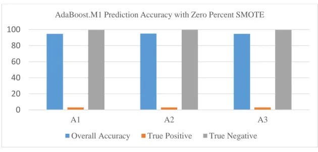
Oversampling is a dimension in the general model due to the scarcity of stuck segments, over
95% of the total data belong in the majority class (figure 2). Most classifiers will unfortunately choose to
predict all testing instances as not stuck as it would give the best overall accuracy, >95%, resulting in 0%
oversampling is used to boost the number of minority class instances in the training set and, hence, true
positive prediction accuracy.
Figure 2: Number of Not Stuck Instances versus Stuck Instances
Figure 3: Accuracy without Oversampling
The oversampling dimension consists of 2 oversampling algorithms: SMOTE and resample.
SMOTE, Synthetic Minority Oversampling Technique, is a minority class oversampling algorithm that
generalizes the minority class space by generating synthetic minority class instances [2]. Resample
algorithm resamples with replacement already present minority class instances; it does not generate any
synthetic minority class instances. Therefore, resample algorithm serves as an excellent baseline for
detecting whether synthetic instances improves classification accuracy.
0
20
40
60
80
100
A1 A2 A3
AdaBoost.M1 Prediction Accuracy with Zero Percent SMOTE
There are 3 classifiers in the classifier dimension. J48 decision tree is the classifier used in
Carter’s research and an excellent difficulty classifier, especially for true negative predictions.
AdaBoost.M1 with decision stump is a new classifier chosen for this research. It can predict difficult to
predict instances by training an ensemble of classifiers, in this case decision stumps, on weighted training
dataset. Each decision stump is trained and validated with the training set. The incorrectly predicted
instances’ weights are increased after prediction, emphasizing the instance. The newly weighted training
instances are then used to train the next decision stump in the ensemble [3]. The collective power of the
ensemble in AdaBoost.M1 should allow it to correctly predict more minority class instances during
testing. Bagging with decision stump is another addition in the current research. Bagging has an ensemble
of classifiers, also decision stumps, similar to AdaBoost.M1. But, it instead seeks to reduce variance by
dividing the training set into “bags” created by resampling with replacement. Each bag serves as the
training set for a decision stump in the ensemble. Bagging prevents over fitting to the training dataset and
allows for better classifier generalization power [4].
Two model validation techniques comprise the evaluation dimension of the general model.
Tenfold cross-validation (10x CV) is a standard analysis technique for evaluating the accuracy of
classifiers on test instances. Leave-one-out participant (LOOP) is used to give a realistic indicator of
prediction accuracy. LOOP model validation technique is as follow:
1. The classifier for each scheme is trained on all participant minus one participant.
2. The classifier is then tested on the data of participant that was left out of the training set.
3. Repeat steps 1-2 for all participants.
LOOP is a more realistic indicator of prediction accuracy as rarely are user’s Eclipse events
distributed as evenly as those in cross-validation. CV divides the entire dataset randomly into different
groups or folds. Nine of ten folds are used to train the classifier and the last one is used to test the
accuracy of the classifier. Unfortunately, if any participant is an outlier, the outlier would have been split
set because it is trained on a portion of the outlier data. However, in real world situations, the testing
users’ data distributions are not present in the training set. Therefore, LOOP best mimics the introduction
of a new user to the classifiers.
Two additional dimensions not in the general model are the startup lag and segment length. Both
are fixed for all scheme families. Segment length refers to the number of events per segment. The single
segment is converted to ratios of each classifier attribute and serves as the classifier dataset instances. The
startup lag prevents any erratic eclipse startup events from being recorded in the segments and used as
classifier dataset instances.
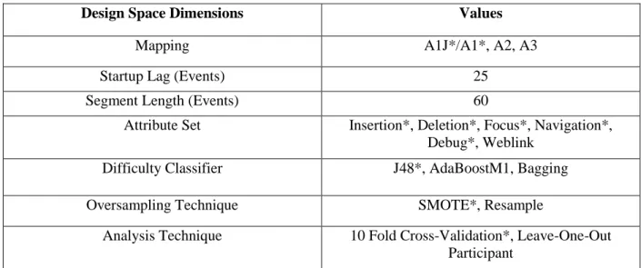
Table 3 is a summary of the design space dimensions and their respective values.
Design Space Dimensions Values
Mapping A1J*/A1*, A2, A3
Startup Lag (Events) 25
Segment Length (Events) 60
Attribute Set Insertion*, Deletion*, Focus*, Navigation*,
Debug*, Weblink
Difficulty Classifier J48*, AdaBoostM1, Bagging
Oversampling Technique SMOTE*, Resample
Analysis Technique 10 Fold Cross-Validation*, Leave-One-Out
Participant
Table 4: Summary of Design Space Dimensions and Their Respective Values
* denotes present in Carter’s original research
Much of the model validation techniques, filters, and classifier used in this research is from
WEKA. WEKA is a machine learning toolkit that provides a platform for testing difficulty prediction
schemes [5].
4. Analysis
Before analysis was conducted on the schemes, we ensured that our analysis environment was
families A1 and A0 with J48 decision tree in the current environment. As mentioned before, A1 and A0
are Carter’s A1J and A0J but applied to all 17 participants.
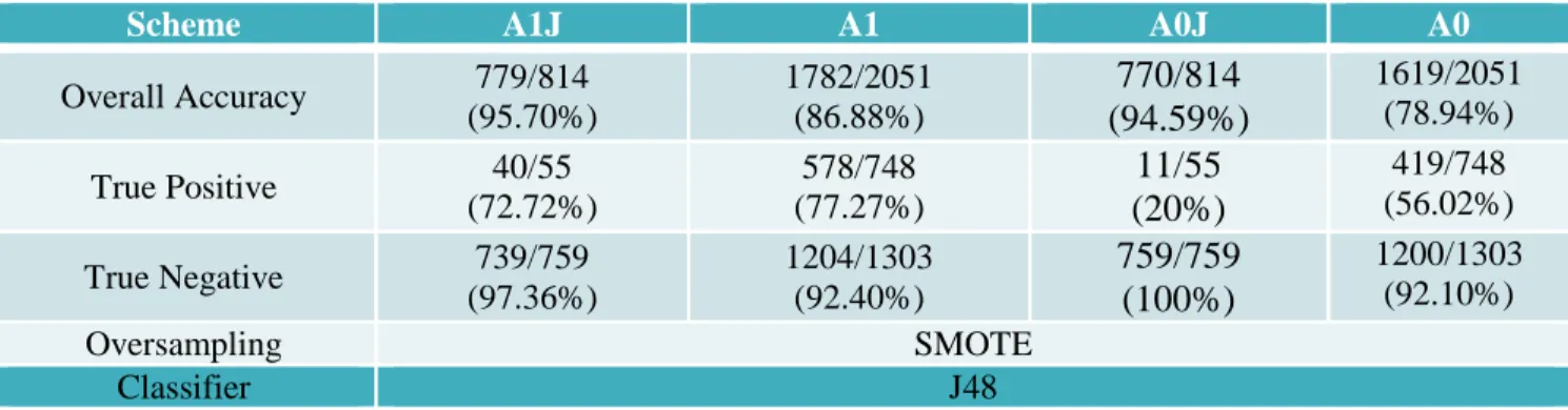
Scheme A1J A1 A0J A0
Overall Accuracy 779/814
(95.70%) 1782/2051 (86.88%)
770/814
(94.59%)
1619/2051 (78.94%)True Positive 40/55
(72.72%) 578/748 (77.27%)
11/55
(20%)
419/748 (56.02%)True Negative 739/759
(97.36%) 1204/1303 (92.40%)
759/759
(100%)
1200/1303 (92.10%)Oversampling SMOTE
Classifier J48
Table 5: Carter's Schemes under the Current Environment
Due to the greater quantity of stuck instances, both A0 and A1 have higher true positive accuracy
than A0J and A1J, respectively. However, as stuck instances are more numerous in A0 and A1, the lower
true positive prediction accuracies have pronounced negative impact on the overall prediction accuracies.
The decline of true negative accuracy as participants increased is due to the more generalized
classifier created as a result of bigger training dataset. Before, since stuck instances were the vast
minority, the difficulty classifiers of A0J and A1J overfitted to the majority class to achieve high true
negative prediction accuracy. However, in A0 and A1, minority class instances are much more numerous,
as a result, the classifiers have less incentive to overfit to majority class as that entails incorrectly
predicting a greater quantity of the now more numerous minority class. Naturally, true negative accuracy
declines.
Therefore, the results are to be expected and we can conclude that our analysis environment is
similar to Jason’s environment.
4A. Attribute Set Analysis
The sole difference between the attribute sets of A1 and A2 is the addition of the weblinks
attribute. Ten-fold cross-validation analysis of scheme family A2 and A1 was conducted with J48
Scheme A1J A1 A2
Overall Accuracy 779/814 (95.70%) 1782/2051 (86.88%) 1849/2051 (90.15%)
True Positive 40/55 (72.72%) 578/748 (77.27%) 634/748 (84.76%)
True Negative 739/759 (97.36%) 1204/1303 (92.04%) 1215/1303 (93.25%)
Oversampling SMOTE to 50% of
Majority Class
SMOTE to 1000% of Minority Class
SMOTE to 1000% of Minority Class
Classifier J48
Table 6: Varying the Attribute Set with J48 and 10x Cross Validation
A2 is better than A1 for difficulty prediction in every metric, recall that A1 is Carter’s scheme,
A1J, except applied to all 17 participants. Since A2 and A1 only differs in the attribute set dimension, it is
reasonable to conclude that weblinks does indeed positively benefit the prediction accuracy.
Information gain analysis is also conducted on the weblinks attribute. Information gain uses the
Information gain equation, equation 1, to rank each attribute in the dataset by its discriminating power
between instances of stuck and not stuck class.
The ranking is calculated with WEKA’s information gain attribute evaluator and ranker and
tabulated in table 6.
A1 A2 A3
Weblinks - 2 1
Deletion 2 1 2
Debug 1 5 3
Focus 4 3 5
Insertion 3 4 4
Navigation 5 6 6
Table 7: Information Gain Ranking Among the Attribute Sets of Each Scheme
Weblinks is consistently ranked within the top 2 by information gain evaluator. Therefore, we
have a mathematical basis on the positive effect of the weblinks attribute on prediction accuracy.
Since scheme families A2 and A3 varies only in the mapping dimension, we trained J48 trees
with A2 and A3 and used cross-validation to verify the effect of new mapping on prediction accuracy.
Scheme family A2 is superior to A3 in every metric. Therefore, there is no conclusive evidence
that the change in mapping from A2 to A3 results in improvement in classification accuracy. In fact, even
scheme family A1, 86.88% overall and 77.27% true positive accuracy, is superior to A3. We can
conclude that the mapping used in both A1 and A2 is superior to A3’s M3 mapping.
5. Leave-One-Out Participant (LOOP)
As stated before, 10 fold cross validation is not a good real world indicator of classifier accuracy.
Therefore, attribute set and mapping analysis were also conducted with leave-one-out participant model
validation. The classifier, J48, and the oversampling technique, SMOTE, remained constant as before.
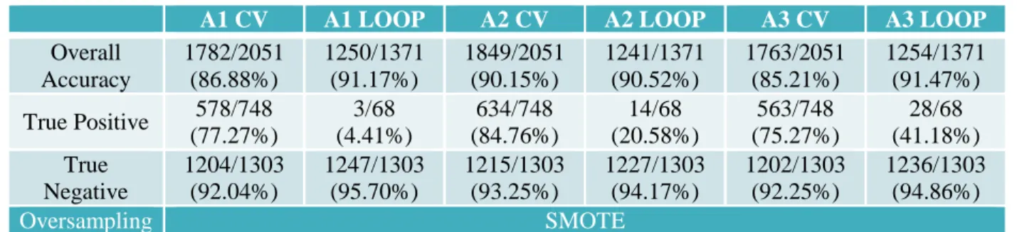
A1 CV A1 LOOP A2 CV A2 LOOP A3 CV A3 LOOP
Overall Accuracy 1782/2051 (86.88%) 1250/1371 (91.17%) 1849/2051 (90.15%) 1241/1371 (90.52%) 1763/2051 (85.21%) 1254/1371 (91.47%) True Positive 578/748
(77.27%) 3/68 (4.41%) 634/748 (84.76%) 14/68 (20.58%) 563/748 (75.27%) 28/68 (41.18%) True Negative 1204/1303 (92.04%) 1247/1303 (95.70%) 1215/1303 (93.25%) 1227/1303 (94.17%) 1202/1303 (92.25%) 1236/1303 (94.86%) Oversampling SMOTE
Table 9: Leave-One-Out Participant Result vs 10x CV Result
Compared to 10 fold cross-validation, LOOP gives a much more pessimistic outlook of true
positive prediction accuracy. Scheme A1’s true positive accuracy with LOOP decreased substantially
compared to with CV. A2 and A3 also experienced decrease in true positive prediction accuracy. This
Scheme Family A2 A3
Mapping A1 A3
Overall Accuracy 1849/2051 (90.15%) 1763/2051 (85.21%)
True Positive 634/748 (84.76%) 563/748 (75.27%)
True Negative 1215/1303 (93.25%) 1202/1303 (92.25%)
Oversampling SMOTE to 1000% of Minority
Class
SMOTE to 1000% of Minority Class
Classifier J48
demonstrates that the J48 decision tree does not generalize well to minority class space and CV does not
adequately detect this shortcoming.
However, weblinks as a valuable classifier dataset attribute still holds. Scheme families A2 and
A3 are much better in terms of true positive accuracy and have similar overall prediction accuracy
compared to A1. Mapping lead to a major difference between scheme family A2 and A3; true positive
prediction accuracy increased 2 fold from A2 to A3. A3 also enjoys better overall accuracy compared to
A2. Intuitively, CV does not accurately reflect this because A3 with J48 tree has better generalization
power; hence, lower accuracy in cross-validation since it does not attempt to over fit to outliers in the
training set like A1 and A2 does.
We have established that CV cannot be used reliably to assess the prediction accuracy of the
difficulty classifiers in each scheme. Therefore, LOOP is used as the analysis technique for the rest of the
analysis.
5A. Schemes with the Best Accuracy
True positive prediction accuracy is a concern with the J48 decision tree when used with scheme
families A1, A2, and A3. Therefore, we adjusted the classifier dimension and oversampling dimension of
each scheme family to acquire the best true positive accuracy under LOOP. Due to the large number of
possible combinations, we enumerate only the best true positive accuracy achieved with a scheme from
each scheme family here and the respective dimension settings.
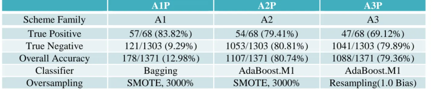
A1P A2P A3P
Scheme Family A1 A2 A3
True Positive 57/68 (83.82%) 54/68 (79.41%) 47/68 (69.12%)
True Negative 121/1303 (9.29%) 1053/1303 (80.81%) 1041/1303 (79.89%)
Overall Accuracy 178/1371 (12.98%) 1107/1371 (80.74%) 1088/1371 (79.36%)
Classifier Bagging AdaBoost.M1 AdaBoost.M1
Oversampling SMOTE, 3000% SMOTE, 3000% Resampling(1.0 Bias)
Table 10: Best True Positive Accuracy Achieved with Each Scheme and Its Dimension Settings
Scheme A2P with AdaBoost.M1 and SMOTE to 3000% achieves the best true positive accuracy
better true positive accuracy, but it overfitted to the minority class space, resulting in extremely low true
negative and overall accuracy. Therefore, scheme A1P is not a reasonable choice in detecting stuck
instances due to the high number of false positives.
A scheme with high overall accuracy is also desired. High overall accuracy corresponds to high
true negative because the majority class vastly outnumbers the minority class. Therefore, a great true
negative is the key to great overall accuracy, but the schemes should also have reasonable true positive
accuracy.
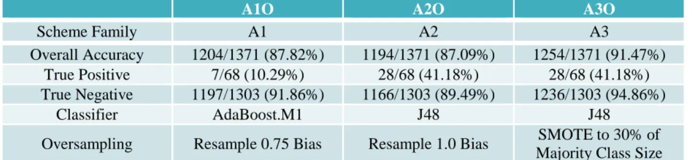
A1O A2O A3O
Scheme Family A1 A2 A3
Overall Accuracy 1204/1371 (87.82%) 1194/1371 (87.09%) 1254/1371 (91.47%)
True Positive 7/68 (10.29%) 28/68 (41.18%) 28/68 (41.18%)
True Negative 1197/1303 (91.86%) 1166/1303 (89.49%) 1236/1303 (94.86%)
Classifier AdaBoost.M1 J48 J48
Oversampling Resample 0.75 Bias Resample 1.0 Bias SMOTE to 30% of
Majority Class Size
Table 11: Scheme with High Overall Accuracy and Reasonable True Positive Accuracy
Scheme A3O with J48 and SMOTE of minority class to 30% of majority class size gives the best
overall accuracy and decent true positive prediction accuracy.
6. Oversampling Analysis
We also need conclusive evidence that the synthetic minority instances generated in SMOTE do
not adversely affect the prediction accuracy. Table 10 details the best of each accuracy metric achieved
with either resample or SMOTE amongst the three schemes families.
Oversampling
Technique Percent
Scheme Family, Classifier
Best Overall Accuracy
SMOTE, 30% of majority class size
1236/1303 (94.86%)
True Pos: 28/68 (41.18%) A3, J48
Resample, 1.0 bias 1186/1303 (91.02%) True Pos: 29/68 (42.65%) A3, J48
Best True Positive Accuracy
SMOTE, 3000% 54/68 (79.41%)
Overall: 1107/1371 (80.74%)
A2, AdaBoost.M1 with Decision Stump Resample, 1.0 bias Overall: 1113/1371 (81.18%) 49/68 (72.06%) A2, AdaBoost.M1 with
Decision Stump Best True Negative
Accuracy
SMOTE, 30% of majority class size
1236/1303 (94.86%)
Resample, 1.0 bias 1186/1303 (91.02%) True Pos: 29/68 (42.65%) A3, J48
Table 12: SMOTE vs Resample
SMOTE wins in each category by slight margins. Therefore, synthetic minority class instances do
not adversely affect the overall and true positive accuracy. In fact, they improve the classifier accuracy on
all fronts.
7. Conclusion and Future Works
We have discovered a much better alternative scheme, A2P, for applications where true positive
accuracy is critical such as API testing. Scheme family A2 with AdaBoost.M1 and SMOTE to 3000% of
minority class size has great true positive prediction accuracy, 79.41%, compared to A1’s 4%. It does so
with a reasonable compromise in true negatives, 80.81% compared to A1’s 95%. This increase in true
positive accuracy can be attributed to the added dataset attribute weblinks, AdaBoost.M1, and SMOTE.
We also have discovered a scheme, A3O, which emphasizes overall accuracy and can be utilized in
applications such as real-time difficulty-based programming collaboration. Scheme family A3 with J48
decision tree and SMOTE to 30% of majority class size has excellent overall accuracy, 91.47%, and
decent true positive accuracy, 41.18%. Its great overall accuracy can be attributed to A3’s M3 mapping
and the addition of the aforementioned weblinks attribute.
As mentioned previously, stuck points can have many sources or barrier types such as design and
syntax issues. We have conducted a preliminary analysis of barrier types and their predictability; the
results are detailed in table 12. Output barrier is the easiest to predict; on the other hand, design and API
barrier type are more often incorrectly predicted. More research on the correlation between barrier type
and prediction accuracy will greatly benefit the difficulty classifier as it can give insights into the
incorrectly predicted stuck instances.
Another area of interest is classification of programmers by experience. Most inexperienced
programmers will be less inclined to use the debugger and generally encounter more difficulty than
debugger and be less susceptible to protracted difficulty. Classifying the users and customizing the
schemes based on experience level will result in reduced variations in the training dataset, leading to
better predictability and higher true positive and overall accuracy.
Difficulty Type Predicted Correctly Percent of Total
Design 8 66.67
Output 8 80.00
API 7 70.00
Appendix A1: Event to Attribute Mapping Common to A1 and A3 Mapping
Figure 4: Debug Mapping for A1 Mapping
Figure 6: Focus Attribute for A1 Mapping
Appendix A2: M1,M2 Mapping for Insertion and Deletion
Figure 8: A1 Mapping for Deletion Attribute
Appendix A3: M3 Mapping for Insertion and Deletion
References
[1] Carter, J. (2014), Automatic Difficulty Detection, in Department of Computer Science. 2014,
University of North Carolina Chapel Hill. p. 201
[2] Nitesh V. Chawla , Kevin W. Bowyer , Lawrence O. Hall , W. Philip Kegelmeyer, SMOTE:
synthetic minority over-sampling technique, Journal of Artificial Intelligence Research, v.16 n.1, p.321-357, January 2002
[3] Freund, Y. & Schapire, R. (1996). Experiments with a new boosting algorithm, Machine Learning: Proceedings of the Thirteenth International Conference, 148–156.
[4] Breiman, L. (1996) Bagging predictors. Machine Learning 26: pp. 123-140