Universit`
a di Milano–Bicocca
Quaderni di Matematica
On the Stability Functional for Conservation Laws
Rinaldo M. Colombo, Graziano Guerra
Stampato nel mese di aprile 2007
presso il Dipartimento di Matematica e Applicazioni,
Universit`a degli Studi di Milano-Bicocca, via R. Cozzi 53, 20125 Milano, ITALIA.
Disponibile in formato elettronico sul sitowww.matapp.unimib.it. Segreteria di redazione: Ada Osmetti - Giuseppina Cogliandro
tel.: +39 02 6448 5755-5758 fax: +39 02 6448 5705
Esemplare fuori commercio per il deposito legale agli effetti della Legge 15 aprile 2004 n.106.
On the Stability Functional for Conservation Laws
Rinaldo M. Colombo
Dipartimento di Matematica Universit`a degli Studi di Brescia
Via Branze, 38 25123 Brescia, Italy
Graziano Guerra
Dip. di Matematica e Applicazioni Universit`a di Milano – Bicocca Via Bicocca degli Arcimboldi, 8
20126 Milano, Italy
April 24, 2007
Abstract
This note is devoted to the explicit construction of a functional de-fined on all pairs ofL1 functions with small total variation, which is
equivalent to theL1distance and non increasing along the trajectories
of a given system of conservation laws. The present definition of this functional does not need any construction of approximate solutions.
2000 Mathematics Subject Classification: 35L65.
Key words and phrases: Hyperbolic Systems of Conservation Laws
1
Introduction
Let the smooth map f: Ω 7→ Rn define the strictly hyperbolic system of conservation laws
∂tu+∂xf(u) = 0 (1.1)
wheret >0,x∈R andu∈Ω, with Ω⊆Rn being an open set.
Most functional theoretic methods fail to tackle these equations, es-sentially due to the appearance of shock waves. Since 1965, the Glimm functional [14] has been a major tool in any existence proof for (1.1) and related equations. More recently, an analogous role in the proofs of contin-uous dependence has been played by the stability functional Φ introduced in [8, 21, 22], see also [4]. The functional Φ has been widely used to prove the
L1–Lipschitz dependence of solutions to (1.1) (and related problems) from initial data having small total variation, see for example [1, 2, 11, 12, 16, 17]. Special cases comprising data with large total variation are considered in [9, 15, 18, 19, 20]. Nevertheless, the use of Φ is hindered by the necessity of introducing specific approximate solutions, namely the ones based either on Glimm scheme [14] or on the wave front tracking algorithm [4, 13]. The
present paper makes the use of the stability functional Φindependent from any kind of approximate solutions.
Namely, we extend the stability functional to all L1 functions with suf-ficiently small total variation. Moreover, we define it in terms of general piecewise constant functions, making it completely independent from the construction of any sort of approximate solutions. Furthermore, using the present definition, we prove its lower semicontinuity.
Taking advantage of the machinery presented below, we also extend the classical Glimm functionals [4, 14] to general L1 functions with small total variation and prove their lower semicontinuity, recovering some of the results in [3], but with a shorter proof.
As a byproduct, the present functional allows to simplify several parts of the cited papers, where the presentation of the stability functional needs to be preceded by the introduction of all the machinery related to Glimm’s scheme or wave front tracking approximations, see for instance [10].
A further expression of the stability functional in terms of the wave measures introduced in [4, § 10.1] is easily available and does not rely on piecewise constant approximations at all. However, with such expression, the proof of the lower semicontinuity is far less direct. Furthermore, any application of this functional is based on approximating the functional eval-uating it on piecewise constant functions and on the lower semicontinuity to pass to the limit. The construction below allows this approach.
The next section introduces the basic notation. Section 3 is devoted to the Glimm functional. The main result is presented in Section 4. The final Appendix contains a technical proof added for the sake of completeness, but not necessary for Theorem 4.1.
2
Notation
Our general reference for the basic definitions related to systems of conser-vation laws is [4]. We assume throughout that 0 ∈ Ω and that the flux f
satisfies
(F) f ∈ C4(Ω;Rn) is strictly hyperbolic and each characteristic field is
either genuinely nonlinear or linearly degenerate.
Letλ1(u), . . . , λn(u) be thenreal distinct eigenvalues of Df(u), indexed so
thatλj(u) < λj+1(u) for allj and u. Thej-th right eigenvector is denoted rj(u).
Let σ7→ Rj(σ)(u), respectively σ 7→Sj(σ)(u), be the rarefaction curve,
respectively the shock curve, exitingu. If thej-th field is linearly degenerate, then the parameter σ above is the arc-length. In the genuinely nonlinear case, see [4, Definition 5.2], we chooseσ so that
∂λj ∂σ ¡ Rj(σ)(u) ¢ =kj and ∂λ∂σj ¡ Sj(σ)(u) ¢ =kj,
where k1, . . . , kn can be arbitrary positive fixed numbers. In [4] the choice kj = 1 for all j= 1, . . . , n was used, while in [2] another choice was made to cope with diagonal dominant sources. Introduce thej-Lax curve
σ 7→ψj(σ)(u) = (
Rj(σ)(u) if σ ≥ 0 Sj(σ)(u) if σ < 0
and for σ≡(σ1, . . . , σn), define the map
Ψ(σ)(u−) =ψn(σn)◦. . .◦ψ1(σ1)(u−).
By [4,§ 5.3], given any two statesu−, u+ ∈ Ω sufficiently close to 0, there exists a mapE such that
(σ1, . . . , σn) =E(u−, u+) if and only if u+= Ψ(σ)(u−). (2.1)
Similarly, let the mapS and the vectorq be defined by
u+ =S(q)(u−) =Sn(qn)◦. . .◦S1(q1)(u−) (2.2)
as the gluing of the Rankine - Hugoniot curves.
Let u be piecewise constant with finitely many jumps and assume that TV(u) is sufficiently small. Call I(u) the finite set of points where u has a jump. Let σx,i be the strength of the i-th wave in the solution of the
Riemann problem for (1.1) with datau(x−) andu(x+), i.e. (σx,1, . . . , σx,n) = E¡u(x−), u(x+)¢. Obviously if x6∈ I(u) thenσx,i= 0, for all i= 1, . . . , n.
As in [4,§7.7], A(u) denotes the set of approaching waves inu:
A(u) = ¡ (x, i),(y, j)¢∈¡I(u)× {1, . . . , n}¢2:
x < y and eitheri > j ori=j, thei-th field is genuinely non linear, min©σx,i, σy,j
ª <0
while the linear and the interaction potential, following [14] see also [4, formula (7.99)], are V(u) = X x∈I(u) n X i=1 ¯ ¯σx,i¯¯ and Q(u) = X ((x,i),(y,j))∈A(u)
¯
¯σx,iσy,j¯¯.
Moreover, let
Υ(u) =V(u) +C0·Q(u) (2.3)
whereC0 >0 is the constant appearing in the functional of the wave–front
tracking algorithm, see [4, Proposition 7.1]. Recall thatC0 depends only on
Remark 2.1 The maps defined on ΩN with values in R+ by (u1, . . . , uN) 7→ V³PNα=1uαχ[xα,xα+1[ ´ (u1, . . . , uN) 7→ Q ³PN α=1uαχ[xα,xα+1[ ´
for fixedx1< . . . < xN+1, are Lipschitz continuous. Moreover, the Lipschitz constant of the maps
uα¯ 7→V XN α=1 uαχ[xα,xα+1[ uα¯ 7→Q XN α=1 uαχ[xα,xα+1[
is bounded uniformly inN, α¯ anduα for α6= ¯α.
Finally we define
D∗δ = n
v∈L1(R,Ω) :v is piecewise constant andΥ(u)< δ
o
(2.4) and
Dδ= cl©Dδ∗ª
where the closure is in the strong L1–topology. Observe that D
δ contains
allL1 functions with sufficiently small total variation.
For later use, for u∈ Dδ and η >0, introduce the set Bη(u) =
n
v∈L1(R; Ω):v∈ Dδ∗ and kv−ukL1 < η .
o
. (2.5)
Note that, by the definition of Dδ,Bη(u) is not empty and ifη1 < η2, then Bη1(u)⊆Bη2(u). Recall the following fundamental result, proved in [7]:
Theorem 2.2 Let f satisfy (F). Then, there exists a positive δo such that
the equation(1.1)generates for allδ∈]0, δo[a Standard Riemann Semigroup (SRS)S: [0,+∞[× Dδ7→ Dδ, with Lipschitz constantL.
We refer to [4, Chapters 7 and 8] for the proof of the above result as well as for the definition and further properties of the SRS.
3
The Glimm Functionals
Extend the Glimm functionals to allu∈ Dδ as follows: ¯
Q(u) = lim
η→0+v∈infBη(u)Q(v) and
¯
Υ(u) = lim
η→0+v∈infBη(u)Υ(v). (3.1)
The mapsη →infv∈Bη(v)Q(v) and η →infv∈Bη(v)Υ(v) are non increasing. Thus the limits above exist and
¯
Q(u) = sup
η>0v∈infBη(u)Q(v) and
¯
Υ(u) = sup
We prove in Proposition 3.4 below that ¯Q, respectively ¯Υ, coincides withQ, respectivelyΥ, when evaluated on piecewise constant functions. Moreover,
¯
Qalso coincides with the functional defined in [6, formula (1.15)], see also [4, formula (10.10)]. Preliminarily, we exploit the formulation (3.1) to prove the lower semicontinuity of Q and Υ more directly than in [4, Theorem 10.1, p.203–208], see also [3].
Proposition 3.1 The functionalsQ¯ and Υ¯ are lower semicontinuous with respect to the L1 norm.
Proof. We prove the lower semicontinuity of ¯Υ, the case of ¯Q is analogous. Fix u inDδ. Letuν be a sequence in Dδ converging to u inL1. Define εν =kuν−ukL1+ 1/ν. Fixvν ∈Bεν(uν) so that Υ(vν)≤ inf v∈Bεν(u) Υ(v) +εν ≤Υ¯(uν) +εν. Since kvν −ukL1 ≤ kvν−uνkL1+kuν−ukL1 <2εν,
we deduce thatvν ∈B2εν(u) and
inf v∈B2εν(u) Υ(v) ≤ Υ(vν) ≤ Υ¯(uν) +εν; ¯ Υ(u) = lim ν→+∞v∈Binf2εν(u) Υ(v) ≤ lim inf ν→+∞ ¯ Υ(uν)
completing the proof. ¤
The next proposition contains in essence the reason why the Glimm functionals Q and Υ decrease. Compute them on a piecewise constant function u and “remove” one (or more) of the values attained by u, then the values of bothQ andΥdecrease.
Let u=Pα∈Iuαχ[xα,xα+1[ be a piecewise constant function, with uα ∈
Ω,x1 < x2< . . . < xN+1 andI be a finite set of integers. Then, we say that
u1, u2, . . . , uN is the ordered sequence of the values attained by u and, with
a slight abuse of notation, we denote it by (uα:α∈I).
Proposition 3.2 Letuanduˇbe piecewise constant functions attaining val-ues in Ω. Assume that the ordered sequence of the values attained by u
is (uα:α ∈ I), while the ordered sequence of the values attained by uˇ is
(uα:α∈J), with J ⊆I. Then,
Q(ˇu)≤Q(u) and Υ(ˇu)≤Υ(u).
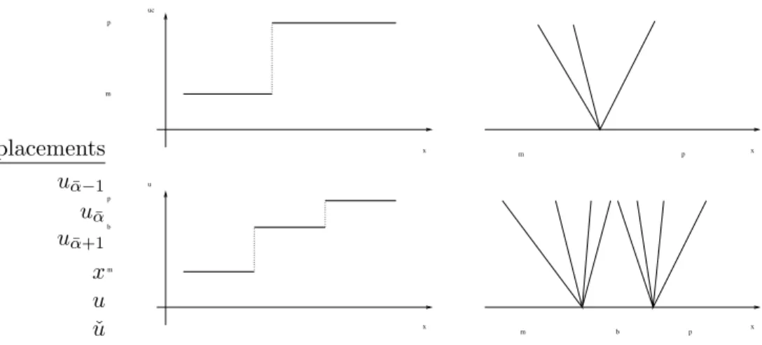
Proof. Consider the case ]I = ]J + 1, see also [4, Step 1, Lemma 10.2]. Then, the above inequalities follow from the usual Glimm interaction esti-mates [14], see Figure 1.
u x x m m b p p p m p b m x x uc PSfrag replacements uα¯−1 uα¯ uα+1¯ x u ˇ u
Figure 1: Proof of Proposition 3.2: uα¯ is attained byu and not by ˇu.
The next lemma is a particular case of [4, Theorem 10.1]. However, the present construction allows to consider only the case of piecewise constant functions, allowing a much simpler proof.
Lemma 3.3 The functionals Q and Υ, defined on D∗
δ, are lower
semicon-tinuous with respect to the L1 norm.
Proof. We consider onlyΥ, the case of Qbeing similar. Letuν be a sequence inDδ∗converging inL1tou=
P
αuαχ[xα,xα+1[∈ Dδ∗
as ν → +∞. By possibly passing to a subsequence, we may assume that
Υ(uν) converges to lim infν→+∞Υ(uν) and that uν converges a.e. to u.
Therefore, for allα= 1, . . . , N, we can select pointsyα ∈]xα, xα+1[ so that
limν→+∞uν(yα) =u(yα) =uα. Define ˇ uν = X α uν(yα)χ[xα,xα+1[.
By Proposition 3.2, Υ(ˇuν) ≤Υ(uν). The convergence uν(yα) → uα for all
α and Remark 2.1 allow to complete the proof. ¤
Proposition 3.4 Let u∈ D∗
δ. Then Q¯(u) =Q(u) and Υ¯(u) =Υ(u).
Proof. We consider onlyΥ, the case of Qbeing similar. Since u∈ D∗
δ, we have that u∈Bη(u) for allη >0 and ¯Υ(u)≤Υ(u).
To prove the other inequality, recall that by the definition (3.1) of ¯Υ, there exists a sequence vν of piecewise constant functions in Dδ∗ such that vν →u inL1 andΥ(vν)→Υ¯(u) as ν →+∞. By Lemma 3.3,
Υ(u)≤lim inf
ν→+∞Υ(vν)≤
¯
Υ(u)
Therefore, in the sequel we write Qfor ¯Q and Υfor ¯Υ.
For the sake of completeness, our next step consists in showing that the functionals Q and Υ coincide with the analogous quantities in [4, Sec-tion 7.7], see also [3, 5]. To this aim, we temporarily denote byVB and QB
the functionals defined therein, moreover we setΥB =VB+C 0·QB.
Proposition 3.5 QB=Q andΥB=Υ.
Proof. We consider onlyΥ, the case of Qbeing similar.
Note first that if u is piecewise constant, then clearly ΥB(u) = Υ(u).
By the definition (3.1) of Υ, there exists a sequence vν of functions in Dδ∗
converging to u in L1 and such that Υ(v
ν) → Υ(u) as ν → +∞. By the
lower semicontinuity ofΥB, see [4, Theorem 10.1], we obtain
ΥB(u)≤lim inf
ν→+∞Υ
B(v
ν) = lim inf
ν→+∞Υ(vν) = limν→+∞Υ(vν) =Υ(u).
Analogously, following [4, Step 3, Theorem 10.1], we may take a sequence
vν of functions in Dδ∗ such that vν → u in L1, VB(vν) → VB(u) and
QB(v
ν) → QB(u) as ν → +∞. Hence, also ΥB(vν) → ΥB(u). Therefore,
along this particular sequence, we may repeat the estimates as above:
Υ(u)≤lim inf
ν→+∞Υ(vν) = lim infν→+∞Υ
B(v
ν) = limν→+∞ΥB(vν) =ΥB(u)
where we applied also Proposition 3.1. ¤
4
The Stability Functional
If δ ∈]0, δo[, choosev,v˜ piecewise constant inD∗
δ. Now, as a first step, we
slightly modify the construction of the stability functional, see [8, 21, 22] and also [4, Section 8.1]. Namely, we construct a similar functional defined on all piecewise constant functions and without any reference to both ε– approximate front tracking solutions and non physical waves.
Define implicitly the functionq(x)≡¡q1(x), . . . qn(x)
¢ by ˜
v(x) =S¡q(x)¢ ¡v(x)¢ withS as in (2.2). We now consider the functional
Φ(v,˜v) = n X i=1 Z +∞ −∞ ¯ ¯qi(x)¯¯Wi(x)dx (4.1) where the weights Wi are defined by
Wi(x) = 1 +κ1Ai(x) +κ1κ2
¡
the constants κ1 and κ2 being defined in [4, Chapter 8]. Denote by σx,i,
respectively ˜σx,i, the size of thei–wave in the solution of the Riemann Prob-lem with datav(x−) and v(x+), respectively ˜v(x−) and ˜v(x+). If thei–th characteristic field is linearly degenerate, thenAi is defined as
Ai(x) =
X n¯
¯σy,j¯¯+¯¯σ˜y,j¯¯: (y, j) such thaty≤x and i < j ≤no +X n¯¯σy,j¯¯+¯¯σ˜y,j¯¯: (y, j) such thaty > x and 1≤j < i
o
.
In the genuinely nonlinear case, let
Ai(x) =
X n¯¯
σy,j
¯
¯+¯¯σ˜y,j¯¯: (y, j) such thaty ≤x andi < j ≤no +X n¯¯σy,j
¯
¯+¯¯σ˜y,j¯¯: (y, j) such thaty > xand 1≤j < io
+ X n¯ ¯σy,i¯¯:y≤xo+X n¯¯˜σy,i¯¯:y > xo ifqi(x) < 0, X n¯¯ σy,i ¯ ¯:y > xo+X n¯¯˜σy,i¯¯:y≤xo ifqi(x) ≥ 0. We stress thatΦis different from the functional Φ introduced in [21, 22] and defined in [4, formula (8.6)]. Indeed, hereall jumps inv or in ˜v are consid-ered. There, on the contrary, exploiting the structure ofε-approximate front tracking solutions, see [4, Definition 7.1], in the definition of Φ the jumps due to non physical waves are neglected when defining the weights Ai and
are considered as belonging to a fictitiousn+1-th family in the definition [4, formula (7.54)] ofQ. To stress this dependence, in the sequel we denote by Φε the stability functional as presented in [4, Chapter 8].
We now move towards the extension of ΦtoDδ. Define
Ξη(u,u˜) = inf©Φ(v,v˜):v ∈Bη(u) and ˜v∈Bη(˜u)ª The mapη→Ξη(u,u˜) is non increasing. Thus, we may finally define
Ξ(u,u˜) = lim
η→0+Ξη(u,u˜) = supη>0Ξη(u,u˜). (4.3)
We are now ready to state the main result of this paper.
Theorem 4.1 The functionalΞ:Dδ× Dδ 7→[0,+∞[defined in(4.3)enjoys
the following properties:
(i) Ξ is equivalent to theL1 distance, i.e. there exists a C >0 such that
for allu,u˜∈ Dδ
1
(ii) Ξ is non increasing along the semigroup trajectories of Theorem 2.2, i.e. for all u,u˜∈ Dδ and for all t≥0
Ξ(Stu, Stu˜)≤Ξ(u,u˜).
(iii) Ξis lower semicontinuous with respect to the L1 norm.
Here and in what follows, we denote byCpositive constants dependent only onf and δ0. We split the proof of the above theorem in several steps.
Lemma 4.2 For all u,u˜∈ D∗
δ, one has Ξ(u,u˜)≤Φ(u,u˜).
We remark that actually Ξ coincides with Φ on all piecewise constant functions. However, the other inequality is rather technical and not neces-sary for the proof of Theorem 4.1. Therefore, we postpone it to the Ap-pendix.
Proof of Lemma 4.2. By the definition (2.5) we have u ∈ Bη(u) and ˜u ∈ Bη(˜u) for allη >0, henceΞη(u,u˜)≤Φ(u,u˜) for all positive η. The lemma
is proved passing to the limitη→0+. ¤
Proposition 4.3 The functional Ξ:Dδ 7→ R is lower semicontinuous with
respect to the L1 norm.
Proof. Fix u and ˜u in Dδ. Let uν, respectively ˜uν, be a sequence in Dδ
converging tou, respectively ˜u. Defineεν =kuν−ukL1+ku˜ν−u˜kL1+ 1/ν.
Then, for each ν, there exist piecewise constant vν ∈Bεν(uν), respectively ˜ vν ∈Bεν(˜uν), such that Φ(vν,v˜ν)≤Ξεν(uν,u˜ν) +εν ≤Ξ(uν,u˜ν) +εν. (4.4) Moreover kvν−ukL1 ≤ kvν −uνkL1 +kuν−ukL1 < 2εν kv˜ν−u˜kL1 ≤ k˜vν −u˜νkL1 +ku˜ν−u˜kL1 < 2εν
so that vν ∈ B2εν(u) and ˜vν ∈ B2εν(˜u). Hence, Ξ2εν(u,u˜) ≤ Φ(vν,v˜ν).
Using (4.4), we obtainΞ2εν(u,u˜) ≤Ξ(uν,u˜ν) +εν. Finally, passing to the liminf for ν→+∞, we have Ξ(u,u˜)≤lim infν→+∞Ξ(uν,u˜ν). ¤
In the next proposition, we compare the functional Φ defined in (4.1) with the stability functional Φε as defined in [4, formula (8.6)]
Proposition 4.4 Let δ >0. Then, there exists a positive C such that for allε >0sufficiently small and for allε-approximate front tracking solutions
w(t, x),w˜(t, x) of (1.1) ¯ ¯ ¯Φ¡w(t,·),w˜(t,·)¢−Φε(w,w˜)(t) ¯ ¯ ¯≤C·ε·°°w(t,·)−w˜(t,·)°°L1.
Proof. Setting ˜w(t, x) =S¡q(t, x)¢ ¡w(t, x)¢and omitting the explicit time dependence in the integrand, we have:
¯ ¯ ¯Φ¡w(t,·),w˜(t,·)¢−Φε(w,w˜)(t) ¯ ¯ ¯≤ Z R n X i=1 ¯ ¯qi(x)¯¯¯¯Wi(x)−Wi(x)¯¯dx . We are thus lead to estimate
¯
¯Wi(x)−Wi(x)¯¯ ≤ κ1¯¯Ai(x)−Ai(x)¯¯+
+κ1κ2¯¯Q(w)−Q(w)¯¯+κ1κ2¯¯Q( ˜w)−Q( ˜w)¯¯.
The second and third summands are each bounded as in [4, formula (7.100)] by C ε. Concerning the former one, recall that Ai and Ai differ only in the absence of non physical waves in Ai. In other words, physical jumps
are counted in the same way in both Ai and Ai while non physical waves
appear in Ai but not in Ai. Therefore, ¯¯Ai(x)−Ai(x)¯¯ is bounded by the sum of the strengths of all non physical waves, i.e. ¯¯Ai(x)−Ai(x)
¯ ¯ ≤ C ε by [4, formula (7.11)]. Finally, using [4, formula (8.5)]:
1 C · ° °v(x)−v˜(x)°°≤Xn i=1 ¯ ¯qi(x)¯¯≤C·°°v(x)−˜v(x)°° (4.5) we obtain ¯ ¯ ¯Φ¡v(t,·),v˜(t,·)¢−Φε(v,v˜)(t) ¯ ¯ ¯≤C ε Z R n X i=1 ¯ ¯qi(x)¯¯dx≤C εkv−v˜k L1
completing the proof. ¤
Proof of Theorem 4.1. The estimates (4.5) show thatΦis equivalent to the
L1 distance between functions inD∗
δ. Indeed, if δ is sufficiently small, then
Wi(x)∈[1,2] for alli= 1, . . . , n and allx∈R, so that 1
To prove(i), fix u,u˜∈ Dδ and choose v∈Bη(u), ˜v∈Bη(˜u). By (4.6), 1 C · ¡ ku−u˜kL1 −2η ¢ ≤ Φ(v,v˜) ≤ 2C·¡ku−u˜kL1+ 2η ¢ 1 C · ¡ ku−u˜kL1 −2η ¢ ≤ Ξη(u,u˜) ≤ 2C·¡ku−u˜kL1+ 2η ¢ .
The proof of(i) is completed passing to the limit η→0+.
To prove (ii), fix u,u˜ ∈ Dδ and η > 0. Correspondingly, choose vη ∈ Bη(u) and ˜vη ∈Bη(˜u) satisfying
Ξ(u,u˜)≥Ξη(u,u˜)≥Φ(vη,v˜η)−η . (4.7)
Let nowε >0 and introduce theε-approximate solutionsvηε and ˜vεη with initial datavε
η(0,·) =vη and ˜vηε(0,·) = ˜vη. Note that forε sufficiently small
Υ ³ vηε(t) ´ ≤ Υε ³ vεη ´ (t) +Cε ≤ Υε(vε η)(0) +Cε ≤ Υ(vη) +Cε < δ+Cε < δ
and an analogous inequality holds for ˜vε
η. Thereforevηε(t),v˜ηε(t)∈ Dδ∗. Here
we denoted with Υε the sumV+C
0Qdefined onε–approximate wave front
tracking solutions (see [4, formulæ (7.53), (7.54)]). We may thus apply Lemma 4.2, Proposition 4.4 and the main result in [4, Chapter 8], that is [4, Theorem 8.2], to obtain Ξ ³ vεη(t),v˜ηε(t) ´ ≤ Φ ³ vεη(t),v˜ηε(t) ´ ≤ Φε ³ vεη,v˜ηε ´ (t) +Cε ° ° °vηε(t)−˜vεη(t) ° ° ° L1 ≤ Φε ³ vεη,v˜ηε ´ (0) +Cεt+Cε ° ° °vηε(t)−v˜ηε(t) ° ° ° L1 ≤ Φ¡vη,v˜η¢+Cεt+Cε ° ° °vηε(t)−v˜ηε(t) ° ° ° L1 +Cε ° °vη−v˜η°° L1.
Recall that as ε → 0 by [4, Theorem 8.1] vε
η(t) → Stvη and ˜vεη(t) → St˜vη.
Hence, Proposition 4.3 and (4.7) ensure that
Ξ(Stvη, St˜vη)≤lim inf ε→0+ Ξ ³ vηε(t),˜vεη(t) ´ ≤Φ¡vη,v˜η ¢ ≤Ξ(u,u˜) +η .
By the choice of vη and ˜vη, we have that vη → u and ˜vη → u˜ in L1 as η → 0+. Therefore, using the continuity of the SRS in L1 and applying
again Proposition 4.3, we may conclude that
Ξ(Stu, Stu˜)≤lim inf
η→0+ Ξ(Stvη, St˜vη)≤Ξ(u,u˜),
completing the proof of (ii). The latter item (iii) follows from
5
Appendix
Proposition 5.1 For all u, u˜ in D∗δ, one has Ξ(u,u˜) = Φ(u,u˜).
Lemma 4.2 provides the first inequality. The proof of the other one follows from the next two lemmas.
Lemma 5.2 The functionalΦ, defined on all piecewise constant functions in D∗
δ, is lower semicontinuous with respect to the L1 norm.
Proof. Fixu,u˜piecewise constant inD∗
δ. Choose two sequences of piecewise
constant mapsuν,u˜ν inD∗δ converging tou,u˜inL1. We want to show that
Φ(u,u˜)≤lim infν→+∞Φ(uν,u˜ν). Call l= lim infν→+∞Φ(uν,u˜ν) and note
that, up to subsequences, we may assume that limν→+∞Φ(uν,u˜ν) =l. By possibly selecting a further subsequence, we also have that both uν and ˜uν
converge a.e. to uand ˜u.
Introduce the functions q= (q1, . . . , qn) andqν = (qν
1, . . . , qnν) by
˜
u(x) =S¡q(x)¢ ¡u(x)¢ and u˜ν(x) =S¡qν(x)¢ ¡uν(x)¢.
withS defined in (2.2). For the computations below, we need the following more explicit notation: fix ¯v(x) ∈ D∗
δ and ¯q piecewise constant, and define
A1(¯v,q¯), . . . ,An(¯v,q¯) through ¡ Ai(¯v,q¯) ¢ (x) = X n¯¯σ¯y,j ¯
¯: (y, j) such thaty≤xand j > io +X n¯¯σ¯y,j
¯
¯: (y, j) such that y > xand j < io for the linearly degenerate case, while for the genuinely nonlinear case:
¡
Ai(¯v,q¯)
¢
(x) = X n¯¯σ¯y,j
¯
¯: (y, j) such thaty≤x and j > io +X n¯¯σ¯y,j¯¯: (y, j) such thaty > xand j < i
o + X n¯
¯σ¯y,i¯¯: (y, i) such that y≤xo if ¯qi(x) < 0 X n¯¯ ¯ σy,i ¯ ¯: (y, i) such that y > xo if ¯qi(x) ≥ 0 ³ ˜ Ai(¯v,q¯) ´ (x) = X n¯¯σ¯y,j ¯
¯: (y, j) such thaty≤x and j > io +X n¯¯σ¯y,j
¯
¯: (y, j) such thaty > xand j < io
+ X n¯¯ ¯
σy,i¯¯: (y, i) such that y≤x
o
if ¯qi(x) > 0 X n¯
¯σ¯y,i¯¯: (y, i) such that y > xo if ¯qi(x) ≤ 0 where, usingE as in (2.1),
(¯σx,1, . . . ,σ¯x,n) =E
¡ ¯
Remark that ¡Ai(¯v,q¯)¢(x) and ³
˜
Ai(¯v,q¯) ´
(x) are Lipschitz function of the values assumed by ¯v (for fixed shock positions). Finally introduce also
¡ Bi(¯v,q¯)¢(x) = ¡Ai(¯v,q¯)¢(x) +κ2Q(¯v) ³ ˜ Bi(¯v,q¯) ´ (x) = ³ ˜ Ai(¯v,q¯) ´ (x) +κ2Q(¯v)
And therefore one has:
Φ(u,u˜) = Z R n X i=1 ¯ ¯qi(x)¯¯× × " 1 +κ1 µ¡ Bi(u, q) ¢ (x) + ³ ˜ Bi(˜u, q) ´ (x) ¶# dx Φ(uν,u˜ν) = Z R n X i=1 ¯ ¯qν i(x) ¯ ¯× × " 1 +κ1 µ ¡ Bi(uν, qν) ¢ (x) + ³ ˜ Bi(˜uν, qν) ´ (x) ¶# dx
Let{x1, . . . , xN+1}be the set of the jump points in u and ˜u and write u= N X α=1 uαχ[xα,xα+1[, u˜= N X α=1 ˜ uαχ[xα,xα+1[.
For all α, select yα ∈ ]xα, xα+1[ so that as ν → +∞, the sequence uν(yα)
converges tou(yα) =uα and ˜uν(yα) to ˜u(yα) = ˜uα. Introduce the piecewise constant function ˇuν =
P
αuν(yα)χ[xα,xα+1[. Let ˇ˜uν be defined analogously.
Because of the Lipschitz dependence (for fixed jump positions) ofAi(¯v),
˜
Ai(¯v) andQ(¯v) on the states attained by ¯v we obtain the pointwise limits lim
ν→+∞Bi(ˇuν, q) =Bi(u, q) and ν→lim+∞
˜
Bi(ˇ˜uν, q) = ˜Bi(˜u, q). (5.1)
Claim: there exists a uniformly bounded sequence of positive mapsων with
lim
ν→+∞ων(x) = 0 a.e. inx
such that, with the notation above, the following inequality holds: ¡ Bi(ˇuν, q) ¢ (x)≤¡Bi(uν, q) ¢ (x) +ων(x)
and a similar inequality holds for ˜Bi.
Proof of the claim. Consider only Bi since the case with ˜Bi is similar.
Fix ¯x∈Rand prove the above inequality passing from ˇuν touν recursively
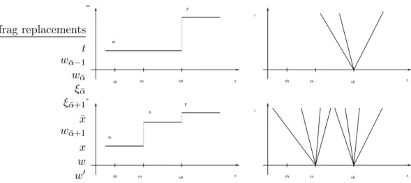
u x xh xa xb x uc m b m p p xb xa xh xh xa xb x x xh xa xb t t PSfrag replacements t wα¯−1 wα¯ ξα¯ ξα+1¯ ¯ x wα+1¯ x w w0
Figure 2: Exemplification of point 2.
1. w0 is obtained from w only shifting the position of the points of jump
but without letting any point of jump cross ¯x. More formally, if w = P αwαχ[ξα,ξα+1[ with ξα < ξα+1, w 0 = P αwαχ[ξα,ξ0 0 α+1[ with ξ 0 α < ξ0α+1 and moreover ¯x∈]ξα, ξα+1[∩ ¤ ξ0 α, ξ0α+1 £ , then ¡ Bi(w0, q)¢(¯x) =¡Bi(w, q)¢(¯x).
Indeed, if all the jumps stay unchanged and no shocks crosses ¯x, then nothing changes in the definition ofAi and Q.
2. w0 is obtained fromwremoving a value attained byw on an interval not
containing ¯x, see Figure 2. More formally, if
w=X α wαχ[ξα,ξα+1[ with ξα < ξα+1 and ¯x6∈ [ξα¯, ξα+1¯ [, then w0 = X α6= ¯α wαχ[ξα,ξα+1[+wα¯−1χ[ξα,ξ¯ α¯+1[ or w0= X α6= ¯α wαχ[ξα,ξα+1[+wα+1¯ χ[ξα,ξ¯ α¯+1[. In this case ¡ Ai(w0, q) ¢ (¯x) +κ2Q(w0)≤ ¡ Ai(w, q) ¢ (¯x) +κ2Q(w).
Indeed, consider for example the case in Figure 2. The two jumps at the pointsξα¯ and ξα+1¯ inw are substituted by a single jump inw0 at the point ξα+1¯ . The points ξα¯ and ξα+1¯ are both to the right of ¯x, therefore the
waves in w0 at the point ξ ¯ α+1 which appear in ¡ Ai(w0, q) ¢ (¯x) are of the same families of the waves inw at the points ξα¯ and ξα+1¯ which appear in ¡
Ai(w, q)
¢
(¯x). Since all the other waves inAi are left unchanged we have
¡ Ai(w0, q)¢(¯x)−¡Ai(w, q)¢(¯x)≤ n X j=1 ¯ ¯ ¯σ0ξα¯+1,j−σξα,j¯ −σξα¯+1,j ¯ ¯ ¯ where σ0 ξα¯+1,j = Ej ¡ w0(ξ ¯ α+1−), w0(ξα+1¯ +) ¢ = Ej(wα¯−1, wα+1¯ ) σξα¯+1,j = Ej ¡ w(ξα+1¯ −), w(ξα+1¯ +) ¢ = Ej(wα¯, wα+1¯ ) σξα¯+1,j = Ej ¡ w(ξα¯−), w(ξα¯+) ¢ = Ej(wα¯−1, wα¯) .
Therefore, the increase in Ai evaluated at ¯x is bounded by the interaction
potential between the waves atξα¯ and those at ξα+1¯ and is compensated by
the decrease inκ2Q, as in the standard Glimm interaction estimates.
3. w0 is obtained fromw changing the value assumed by w in the interval
containing ¯x. More formally, if
w=X α wαχ[ξα,ξα+1[ with ξα < ξα+1 and ¯x∈[ξα¯, ξα+1¯ [, then w0= X α6=¯α wαχ[ξα,ξα+1[+w 0 ¯ αχ[ξα,ξ¯ α¯+1[. In this case ¡ Bi(w0, q) ¢ (¯x)+≤¡Bi(w, q) ¢ (¯x) +C¯¯wα¯−wα0¯ ¯ ¯.
Indeed, this inequality directly follows from the Lipschitz dependence of
Ai(w, q)(¯x) and ofQ(w) on the values attained bywfor fixed jump positions.
For ¯x∈[xα¯, xα+1¯ [ we can pass from uν to to the function wν defined by
wν = X
α6=¯α
uν(yα)χ[xα,xα+1[+uν(¯x)χ[xα,x¯ α¯+1[
applying the first two steps a certain number of times. And we obtain the
estimate ¡ Bi(wν, q) ¢ (¯x)≤¡Bi(uν, q) ¢ (¯x).
Finally with the third step we go fromwν to ˇuν obtaining the estimate:
¡ Bi(ˇuν, q)¢(¯x) ≤ ¡Bi(wν, q)¢(¯x) +C¯¯uν(¯x)−uν(yα¯)¯¯ ≤ ¡Bi(uν, q) ¢ (¯x) +C¯¯uν(¯x)−uν(yα¯) ¯ ¯ ≤ ¡Bi(uν, q) ¢ (¯x) +ων(¯x).
with ων(x) =C N X α=1 ¯ ¯uν(x)−uν(yα)¯¯χ[xα,xα +1[(x).
But a.e. x∈R one has
N X α=1 ¯ ¯uν(x)−uν(yα)¯¯χ[xα,xα +1[(x)→ N X α=1 |uα−uα|χ[xα,xα+1[(x) = 0
proving the claim. Now we write: Φ(u,u˜) =χ1,ν+χ2,ν+χ3,ν+χ4,ν+Φ(uν,u˜ν) , with χ1,ν = Φ(u,u˜) − Z R n X i=1 ¯ ¯qi(x)¯¯ " 1 +κ1 µ ¡ Bi(ˇuν, q) ¢ (x) + ³ ˜ Bi(ˇ˜uν, q) ´ (x) ¶# dx χ2,ν = Z R n X i=1 ¯ ¯qi(x)¯¯κ1 · ¡ Bi(ˇuν, q)¢(x)−¡Bi(uν, q)¢(x) + ³ ˜ Bi(ˇ˜uν, q) ´ (x)− ³ ˜ Bi(˜uν, q) ´ (x) ¸ dx χ3,ν = Z R n X i=1 ¯ ¯qi(x)¯¯κ1 · ¡ Bi(uν, q) ¢ (x)−¡Bi(uν, qν) ¢ (x) + ³ ˜ Bi(˜uν, q) ´ (x)− ³ ˜ Bi(˜uν, qν) ´ (x) ¸ dx χ4,ν = Z R n X i=1 ³¯ ¯qi(x)¯¯−¯¯qν i(x) ¯ ¯´· · " 1 +κ1 µ¡ Bi(uν, qν) ¢ (x) + ³ ˜ Bi(˜uν, qν) ´ (x) ¶# dx .
By the pointwise convergence (5.1) of the integrand, lim
ν→+∞χ1,ν = 0.
Passing to the next summand, note that the claim implies that
χ2,ν≤2C Z R n X i=1 ¯ ¯qi(x)¯¯κ1ων(x)dx and the Dominated Convergence Theorem implies lim inf
ν→+∞χ2,ν ≤0.
Concerning χ3,ν, observe that qiν converges a.e. to q(x), therefore for
sufficiently large and this implies ¡Bi(uν, q)
¢
(x) = ¡Bi(uν, qν)
¢
(x). Hence the integrand inχ3,ν converges a.e. to zero and we have lim
ν→+∞χ3,ν = 0.
Finally theL1convergence ofqν
i toqiimplies limν→+∞χ4,ν = 0, concluding
the proof sinceΦ(uν,u˜ν)→l. ¤
Lemma 5.3 For all piecewise constantu,u˜∈ D∗
δ, Ξ(u,u˜)≥Φ(u,u˜).
Proof. By the definition (4.3) of Ξ, for all u,u˜∈ D∗
δ, there exist sequences vν,˜vνof piecewise constant functions such that forν →+∞we havevν →u,
˜
vν →u inL1 andΦ(vν,v˜ν)→Ξ(u,u˜). Hence, by Lemma 5.2
Φ(u,u˜)≤lim inf
ν→+∞Φ(vν,˜vν) = Ξ(u,u˜),
completing the proof. ¤
References
[1] D. Amadori, L. Gosse, and G. Guerra. Global BV entropy solutions and uniqueness for hyperbolic systems of balance laws. Arch. Ration. Mech. Anal., 162(4):327–366, 2002.
[2] D. Amadori and G. Guerra. Uniqueness and continuous dependence for systems of balance laws with dissipation. Nonlinear Anal., 49(7, Ser. A: Theory Methods):987–1014, 2002.
[3] P. Baiti and A. Bressan. Lower semicontinuity of weighted path length in BV. In Geometrical optics and related topics (Cortona, 1996), vol-ume 32 of Progr. Nonlinear Differential Equations Appl., pages 31–58. Birkh¨auser Boston, Boston, MA, 1997.
[4] A. Bressan. Hyperbolic systems of conservation laws, volume 20 of
Oxford Lecture Series in Mathematics and its Applications. Oxford University Press, Oxford, 2000. The one-dimensional Cauchy problem. [5] A. Bressan and R. M. Colombo. Unique solutions of 2×2 conservation
laws with large data. Indiana Univ. Math. J., 44(3):677–725, 1995. [6] A. Bressan and R. M. Colombo. Decay of positive waves in nonlinear
systems of conservation laws. Ann. Scuola Norm. Sup. Pisa Cl. Sci. (4), 26(1):133–160, 1998.
[7] A. Bressan, G. Crasta, and B. Piccoli. Well-posedness of the Cauchy problem for n×n systems of conservation laws. Mem. Amer. Math. Soc., 146(694):viii+134, 2000.
[8] A. Bressan, T.-P. Liu, and T. Yang. L1 stability estimates for n×n
conservation laws. Arch. Ration. Mech. Anal., 149(1):1–22, 1999. [9] R. M. Colombo and A. Corli. On 2×2 conservation laws with large
data. NoDEA Nonlinear Differential Equations Appl., 10(3):255–268, 2003.
[10] R. M. Colombo and G. Guerra. Hyperbolic balance laws with a dissi-pative non local source. In preparation, 2007.
[11] R. M. Colombo and G. Guerra. Hyperbolic balance laws with a non local source. Communications in Partial Differential Equations, to ap-pear.
[12] R. M. Colombo and G. Guerra. Non local sources in hyperbolic balance laws with applications. In Proceedings of the Eleventh International Conference on Hyperbolic Problems Theory, Numerics, Applications, to appear.
[13] C. M. Dafermos. Polygonal approximations of solutions of the initial value problem for a conservation law. J. Math. Anal. Appl., 38:33–41, 1972.
[14] J. Glimm. Solutions in the large for nonlinear hyperbolic systems of equations. Comm. Pure Appl. Math., 18:697–715, 1965.
[15] G. Guerra. Well-posedness for a scalar conservation law with singu-lar nonconservative source. J. Differential Equations, 206(2):438–469, 2004.
[16] S.-Y. Ha. L1 stability for systems of conservation laws with a
nonreso-nant moving source. SIAM J. Math. Anal., 33(2):411–439 (electronic), 2001.
[17] S.-Y. Ha and T. Yang. L1 stability for systems of hyperbolic
conser-vation laws with a resonant moving source. SIAM J. Math. Anal., 34(5):1226–1251 (electronic), 2003.
[18] M. Lewicka. Well-posedness for hyperbolic systems of conservation laws with large BV data. Arch. Ration. Mech. Anal., 173(3):415–445, 2004. [19] M. Lewicka. Lyapunov functional for solutions of systems of conser-vation laws containing a strong rarefaction. SIAM J. Math. Anal., 36(5):1371–1399 (electronic), 2005.
[20] M. Lewicka and K. Trivisa. On theL1well posedness of systems of
con-servation laws near solutions containing two large shocks.J. Differential Equations, 179(1):133–177, 2002.
[21] T.-P. Liu and T. Yang. A new entropy functional for a scalar conser-vation law. Comm. Pure Appl. Math., 52(11):1427–1442, 1999.
[22] T.-P. Liu and T. Yang. Well-posedness theory for hyperbolic conserva-tion laws. Comm. Pure Appl. Math., 52(12):1553–1586, 1999.