MODELING LONGITUDINAL DATA WITH INTERVAL
CENSORED ANCHORING EVENTS
Chenghao Chu
Submitted to the faculty of the University Graduate School in partial fulfillment of the requirements
for the degree Doctor of Philosophy
in the Department of Biostatistics, Indiana University
Accepted by the Graduate Faculty, Indiana University, in partial fulfillment of the requirements for the degree of Doctor of Philosophy.
Doctoral Committee
March 1, 2018
Ying Zhang, Ph.D., Co-chair
Wanzhu Tu, Ph.D., Co-chair
Chunyan He, Sc.D.
c 2018 Chenghao Chu
DEDICATION
To: Nan Jia,
Natalie Chu and Justin Chu, and my parents.
ACKNOWLEDGMENTS
I am sincerely thankful to Dr. Ying Zhang and Dr. Wanzhu Tu, both of whom are my mentors and friends. As mentors, their solid knowledge, keen insights, and professional skills have benefitted me as a student, and will continue benefitting me as a statistician. As friends, their generosity and intelligence helped me out of those difficult times, and encouraged me to explore new paths in my life-journey.
I am also thankful to Dr. Chunyan He and Dr. Giorgos Bakoyannis for valuable comments on my research, and kindly serving on my research committee.
It has been an enjoyable four years of studying and living in my department. I thank everyone for the friendship.
Dr. Malaz Boustani and the Center for Health Innovation and Implementation Science (CHIIS) provided me financial support and various opportunities to practice my statistical training. I greatly appreciate their generosity.
I thank my parents and my wife for all the support, and my children for all the joy.
Chenghao Chu
MODELING LONGITUDINAL DATA WITH INTERVAL CENSORED ANCHORING EVENTS
In many longitudinal studies, the time scales upon which we assess the primary out-comes are anchored by pre-specified events. However, these anchoring events are often not observable and they are randomly distributed with unknown distribution. Without direct observations of the anchoring events, the time scale used for analysis are not available, and analysts will not be able to use the traditional longitudinal models to describe the temporal changes as desired. Existing methods often make either ad hoc or strong assumptions on the anchoring events, which are unverifiable and prone to biased estimation and invalid inference.
Although not able to directly observe, researchers can often ascertain an in-terval that includes the unobserved anchoring events, i.e., the anchoring events are interval censored. In this research, we proposed a two-stage method to fit commonly used longitudinal models with interval censored anchoring events. In the first stage, we obtain an estimate of the anchoring events distribution by nonparametric method using the interval censored data; in the second stage, we obtain the parameter esti-mates as stochastic functionals of the estimated distribution. The construction of the stochastic functional depends on model settings. In this research, we considered two types of models. The first model was a distribution-free model, in which no parametric assumption was made on the distribution of the error term. The second model was
that the origin of the time scale for analysis was interval censored. For the pur-pose of large-sample statistical inference in both models, we studied the asymptotic properties of the proposed functional estimator using empirical process theory. Theo-retically, our method provided a general approach to study semiparametric maximum pseudo-likelihood estimators in similar data situations. Finite sample performance of the proposed method were examined through simulation study. Algorithmically effi-cient algorithms for computing the parameter estimates were provided. We applied the proposed method to a real data analysis and obtained new findings that were incapable using traditional mixed-effects models.
Ying Zhang, Ph.D., Co-Chair Wanzhu Tu, Ph.D., Co-Chair
TABLE OF CONTENTS
LIST OF TABLES . . . x
LIST OF FIGURES . . . xi
Chapter 1 Introduction . . . 1
Chapter 2 Introduction to vector calculus . . . 4
2.1 Vector calculus . . . 4
Chapter 3 A short introduction to empirical process theory . . . 9
3.1 Stochastic process and weak convergence . . . 9
3.2 Empirical process, Glivenko-Cantelli class, and Donsker class . . . 12
3.3 Some Donsker classes . . . 16
3.4 A general theorem . . . 21
Chapter 4 A distribution-free model with interval censored anchoring points 27 4.1 Model formulation and estimation . . . 27
4.2 Asymptotic property . . . 31
4.3 Simulation study . . . 43
4.4 Analysis of pubertal skeletal growth data . . . 48
Chapter 5 Mixed-effects model with interval censored anchoring points . . 56
5.1 Estimation with with interval-censored anchoring points . . . 57
5.1.1 Parameter estimation . . . 57
5.1.2 Asymptotic property . . . 59
5.2.1 Linear mixed-effects model with interval censored anchoring
points . . . 70
5.2.2 Computation . . . 71
5.2.3 Derivation of the formula in Section 5.2.1 . . . 75
5.3 Simulation study . . . 82
5.4 Analysis of pubertal weight growth data . . . 91
Chapter 6 An R function for fitting linear mixed-effects model with interval censored anchoring points . . . 96
6.1 Nonparametric maximum likelihood estimation of the anchoring point distribution . . . 96
6.2 A hybrid algorithm combining Fisher-Scoring algorithm and EM-algorithm . . . 101
6.3 A user-friendly function . . . 111
Chapter 7 Summary . . . 117
BIBLIOGRAPHY . . . 119 CURRICULUM VITAE
LIST OF TABLES
4.1 Simulation result for wider censoring intervals. . . 45 4.2 Simulation result for narrower censoring intervals. . . 46 4.3 Empirical relative efficiency: proposed method vs knowing F0. . . . 47
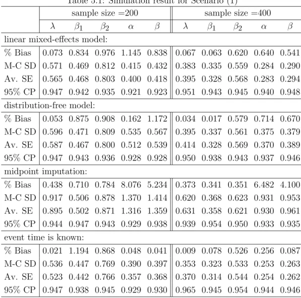
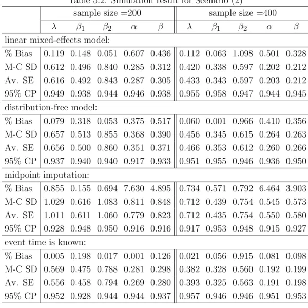
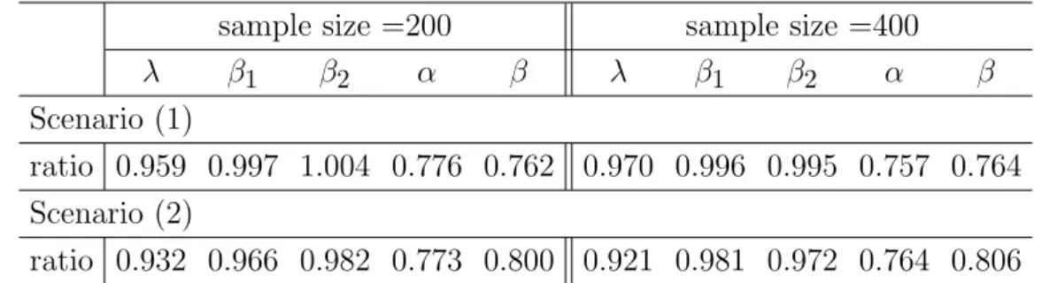
5.1 Simulation result for Scenario (1) . . . 85 5.2 Simulation result for Scenario (2) . . . 86 5.3 Ratio of Monte Carlo standard deviations of linear mixed-effects model
vs distribution-free model . . . 87 5.4 Ratio of Monte Carlo standard deviations of linear mixed-effects model
vs the model knowing true event time . . . 88 5.5 Simulation result for Scenario (1) with mixture normal errors . . . . 89 5.6 Simulation result for Scenario (2) with mixture normal errors . . . . 90 5.7 Ratio of Monte Carlo standard deviations of linear mixed-effects model
vs distribution-free model with mixture normal errors . . . 91 5.8 Ratio of Monte Carlo standard deviations of proposed model vs the
model knowing true event times with mixture normal errors . . . 91 5.9 Parameter estimates . . . 94
LIST OF FIGURES
4.1 Peak growth periods in 360 children . . . 49
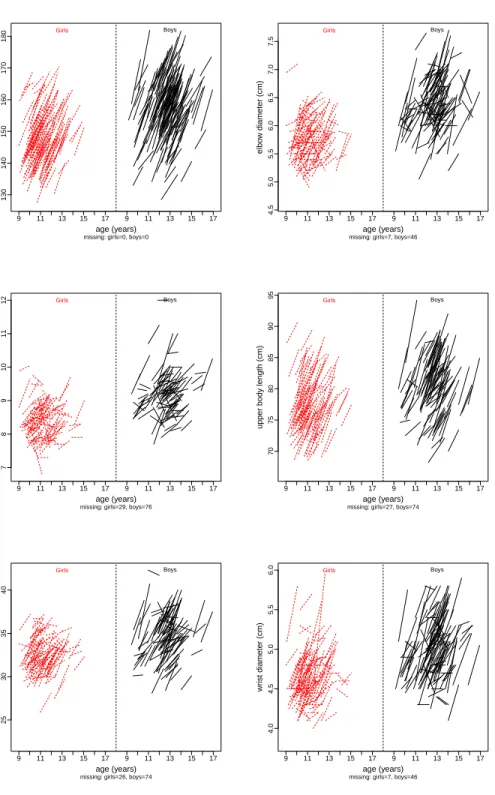
4.2 Observed data . . . 50
4.3 The estimated CDFs of F0 for males and females . . . 51
4.4 The fitted anchoring point models. . . 52
Chapter 1
Introduction
In many biomedical investigations, the process under study is known to be anchored by certain event of clinical significance. We call such event as anchoring event and its timing of occurrence as anchoring point. Researchers are often interested in quantify-ing the patterns of the process around the anchorquantify-ing events. For example, oncologists want to assess the rates of neoplastic growth immediately following the initial tu-morigenesis or subsequent tumor recurrence (Fournier et al., 1980; Spratt et al., 1993; Carter et al., 1989). Human growth researchers want to evaluate the rates of skele-tal changes before and after puberskele-tal growth spurt (PGS), i.e., the time at which a child’s height increase reaches its maximum velocity (Tanner and Whitehouse, 1976). In these examples, tumorigenesis/recurrence and PGS only function as events that anchor the time scale for the analysis. When these events are observed, the time scale for analysis is available, and usual mixed-effects models (Laird and Ware, 1982) or subject-specific smoothing models (Durb´an et al., 2005) can be devised to model the trajectory of the process under investigation. In reality, however, the anchoring events are not always directly observed and the individual anchoring points should be regarded as a random quantity with an unknown distribution. In such situation, the time scale for analysis is not available, and all traditional methods can not be directly applied, because the time scale for building those models is no longer available.
We are interested in the situation that the anchoring points are interval cen-sored. Such situation is abundant in real life studies, because investigators are usu-ally able to determine the time intervals within which the anchoring events occur. In literatures, parametric joint models were proposed to analyze data with interval censored anchoring events (van den Hout et al., 2013; Robinson et al., 2010). Im-putation methods were also often seen in practice (Shankar et al., 2005; Tu et al., 2009). By assuming all subjects share the same anchoring point, changing-point models (Muller, 1992) was also proposed. But these methods suffer from the follow-ing fundamental limitations: (1) The parametric assumptions are not easy to verify, and are prone to biased estimation; (2) They are unable to accommodate the un-certainty associated with the estimation of the anchoring point for each individual subject. Recently, Zhang et al. (2016) proposed a robust nonparametric estimator for post-PGS pubertal growth, which was anchored by the unobservable PGS. Their ap-proach was purely nonparametric and they showed that the estimator was consistent. Although no asymptotic normality theory was established to allow an asymptotic inference procedure, their two-stage estimation method shed a light to overcome the aforementioned difficulties in these problems. First, it completely side-stepped the difficulty of estimating the subject specific anchoring points; Second, by regarding the model estimates as stochastic functionals of the estimated anchoring point distribu-tion, asymptotic distributions of the model estimates were possible to study through the empirical process theory.
In this research, we adopted the two-stage functional estimation method from Zhang et al. (2016) to analyze longitudinal data involving interval censored anchoring
first model was distribution-free in the sense that we did not make any parametric assumption on the outcomes. The advantages of this method were the robustness against the unknown distribution of the outcomes, and the numerical convenience in computing the parameter estimates. But it completely ignored the possible corre-lations among the repeated measures within the same subject. Therefore, a second model based on mixed-effects models was proposed. Although statistically more effi-cient, the second model was numerically more complicated than the first model. For both models, we showed under mild regularity conditions that the model estimates were asymptotically normally distributed with√n-convergence rate, and hence statis-tical inference can be conducted for large samples. Simulation studies were conducted to validate the asymptotic properties, as well as to examine the good finite sample performance. Real data analysis were presented to illustrate the application of the proposed method.
The thesis is structured as follows. Chapter 2 reviews necessary vector cal-culus needed for studying linear mixed-effects models. Chapter 3 briefly reviews the empirical process theory that is used for this research. In addition, we provide a general theory that is useful to study the large sample property of model estimates, obtained from the proposed two-stage functional estimation procedure. With these theoretic preparations, the distribution-free model is studied in Chapter 4, and the mixed-effects model is studied in Chapter 5. The proposed methods are implemented using R software in Chapter 6. A summary of this work is provided in Chapter 7.
Chapter 2
Introduction to vector calculus
The likelihood function of a mixed-effects model naturally takes the covariance matrix G of the random effects as an argument. To calculate the estimating equations, we must calculate the derivatives with respect to the entries of G. One could simply parameterize G by its entries, or some entries since G is symmetric and possibly structured. However, taking derivatives with respect to one entry at a time may be difficult since the likelihood function is complicated, especially when G has a large size. Vector calculus is a mathematical tool that arranges all partial derivatives in an organized manner, so that it takes partial derivatives with respect to all the parameters in G in one step. In other words, vector calculus is a convenient device that helps to calculate the estimating equations for mixed-effects models.
In this chapter, we review some results in vector calculus. These results are well known and can be found in any textbook on vector calculus. We state them in lemmas for the convenience of reference in later chapters.
2.1 Vector calculus
By “vector” we always mean a column vector. If V is a vector, its transpose is denoted byVt, which is a row vector. Both column and row vectors are also regarded as matrices.
In many situations, a scalar function f takes a matrix G = xij
m×n as an argument. Indeed, f is a multivariate function on the variables {xij
1≤ i≤ m,1≤
j ≤n}, and hence it makes sense to define the gradient off with respect to thexij’s. It is more convenient to write the gradient ∇Gf in a matrix form as
∇Gf = ∂f ∂xij m×n .
In particular, if X = (x1,· · · , xn) is a row vector, then we write the gradient
∇Xf = ( ∂f
∂x1,· · · , ∂f ∂xn
)
as a row vector; ifX = (x1,· · · , xn)t is a column vector, we write the gradient
∇Xf = ∂f ∂x1 ,· · · , ∂f ∂xn t
as a column vector. For a multivariate functionF = (f1(X),· · · , fm(X))t,regardless of X being a row or column vector, we always denote the Jacobian of F as
∇XF = ∂fi ∂xj m×n
which is a matrix. Some useful properties of these operations are summarized in the following lemma, whose validity can be easily checked.
• Product rule. For scalar function f and multivariate functions F, G:
∇(FTG) = Gt(∇F) +Ft(∇G) and ∇(f G) =G(∇f) +f(∇G).
• For a constant matrix A and a multivariate function F,
∇(AF) =A∇F.
• Chain rule. For a multivariate function G(X) = g1(X),· · ·, gm(X)t and a
multivariable function F(y1,· · · , ym),
∇X(F ◦G) =∇YF
Y=G(X)· ∇XG.
• For scalar functions f and h of matrix variable G,
∇G(f h) = f(∇Gh) +h(∇Gf) and ∇G(f(h(G))) = f0(h(G))(∇Gh).
Another often seen situation is when a matrix is a function of a variable t. That is,A(t) = aij(t)
, where the entries aij(t) are functions of t. The derivative of A(t) is defined as the following matrix.
A0(t) = dA(t) dt = da ij(t) dt .
Lemma 2.1.2. (Wand, 2002, Section 3) For differentiable matrices A(t) and B(t):
(A(t) +B(t))0 =A0(t) +B0(t), (A(t)B(t))0 =A(t)B0(t) +A0(t)B(t).
The following well-known result is very useful when deriving estimating equa-tions of longitudinal models. A short proof is provided for self-completeness.
Lemma 2.1.3. (Wand, 2002, Section 3) If A(t) is nonsingular, then 1. (Jacobi’s Formula) dtd(det(A(t))) =det(A(t))·T rA(t)−1dAdt(t),
2. (A−1(t))0 =−A−1(t)A0(t)A−1(t).
Proof. For the Jacobi’s Formula, we have the following direct calculations.
d
dt(det(A(t))) = lim
h→0
det(A(t+h))−det(A(t)) .
h
= det(A(t)) lim h→0
det(A(t)−1A(t+h))−1.h
= det(A(t)) lim h→0
det(I+hA(t)−1ddtA +h2A∗)−1.h by Taylor expanson, where A∗ is a bounded matrix onh.
= det(A(t)) lim h→0
1 +h·T r(A(t)−1ddtA) +O(h2)−1.h
For the derivative of the inverse matrix, we apply Lemma 2.1.2 to have the following calculations. I =A(t)A−1(t) =⇒ ddtI = d(A(t)A −1(t)) dt =⇒ O =A0(t)A−1(t) +A(t)A−1(t)0 =⇒ (A−1(t))0 =−A−1(t)A0(t)A−1(t).
Chapter 3
A short introduction to empirical process theory
The study of asymptotic properties in our work relies heavily on the modern empir-ical process theory (Dudley, 1984; Pollard, 1990; van der Vaart and Wellner, 1996; Kosorok, 2007). In this chapter we first review some important definitions and results in empirical process theory, and then present a useful lemma that helps to study the Donsker property of a class of functions. We also provide a general theorem, which provides sufficient conditions for a sequence of stochastic functionals to converge.
By “map” we mean a map between sets. By “metric space” we mean a set together with a notion of distance. By “measurable space” we mean a set together with aσ-algebra, i.e., there is a notion of measurable sets. By “probability space” we mean a set together with a probability measure, i.e, there is a notion of probability of each measurable set. Note that for any metric space, we have a notion of “open sets” (i.e., a topology), and hence a notion of “Borelσ-algebra” as the one generated by the open sets. In other words, any metric space (indeed, topological space) is naturally a measurable space, equipped with the Borel σ-algebra.
3.1 Stochastic process and weak convergence
There are three commonly used equivalent definitions of a stochastic process. Recall that ad-dimensional random variable on a probability space Ω is a measurable func-tion X : Ω → Rd. Let T be a set. The first definition of stochastic process simply
regards a stochastic process Γ on Ω indexed byT as a collection of random variables on Ω :
Γ ={Xt : Ω→Rd t∈T}.
In different applications, different correlation structures among these random vari-ables can be further imposed.
A second equivalent definition of a stochastic process Γ on Ω indexed by T is to be a map between sets
Γ :T ×Ω→Rd,
which sends (t, ω) to Xt(ω), such that each restriction Xt, t ∈ T, is a measurable function on Ω. Note that we treat the indexing set T simply as a set without any possible extra structure, such as symmetry or topology.
There is a third equivalent definition. Following Holden et al. (1996, Section 2.1), it is intuitively helpful to think ω ∈ Ω as a particle, t ∈ T as time, and Xt(ω) as the position of the particle ω at time t. If we fix ω and let t vary in T, we get a sample path:
pω : T →Rd; t 7→Xt(ω).
So a stochastic process on Ω can also be identified as a “measurable” function from the probability space Ω to the space of functions T → Rd, denoted as (Rd)T. The
σ-algebra on (Rd)T is generated by the sets:
At1,···,t
k;B1,···,Bk = {f :T →R
d
Each of the above three equivalent definitions has its advantages in different situations. The third definition makes it easier to define weak convergence of a se-quence of stochastic processes. For a general discussion of weak convergence, we refer the readers to Pollard (2012, Chpater 5). In this section, we define weak convergence of stochastic processes when there is a metric, denoted as k · k, on the space (Rd)T. For example, in most of the problems in this research, the metric is given by the supremum norm k · k∞ on (Rd)T.
Definition 3.1.1. (Kosorok, 2007, Section 7.2.1) Let Γ1,· · · ,Γn,· · · be a se-quence of stochastic processes on Ω indexed by T with values in Rd. The sequence is called weakly convergent to a stochastic process Γ, denoted as
{Γii= 1,· · · }=⇒Γ,
if for every bounded continuous function φ : (Rd)T → R, the sequence of random variables {φ(Γi)i = 1,2,· · · } converges to φ(Γ) in distribution. The σ-algebra on (Rd)T is the Borel algebra associated with the metric on (Rd)T.
Example 3.1.2. (1) A random variable can be thought as a stochastic process indexed by one point. A sequence of random variables {Xi
i= 1,· · · }weakly converges to X, viewed as stochastic processes, if and only if they converge toX in distribution, viewed as random variables. This is a special case of the famous Portmanteau Theorem (Klenke, 2008).
(2) A Gaussian process is a stochastic process such that the random vector
Xt1,· · · , Xtk is multinormal for any finite number of points t1,· · · , tk. If {Γi i=
t1,· · · , tm, the sequence of random vectors {(Γi|t1,· · · ,Γi|tm)
i = 1,· · · } converges in distribution to the multinormal random vector (Γt1,· · · ,Γtm). The converse is true
only under certain conditions, such as “tightness” (Kosorok, 2007, Section 7.1).
3.2 Empirical process, Glivenko-Cantelli class, and Donsker class
An empirical process indexed by T is a stochastic process that is defined through random samples (Kosorok, 2007, Page 9). This general definition is rather abstract. In all applications in this thesis, we consider the following special type of empirical processes. Let Ω ⊂ Rd be a probability space with probability measure P. If f is a random variable on Ω, we write the expectation of f as Pf. Let F be a class of measurable functions on Ω, then we have a deterministic functional on F:
P : F →R; f 7→Pf.
Now, if we have a random sample of size n on Ω, denoted as {ωii= 1,· · · }, we can define an empirical measure Pn on Ω as
Pn(A) = 1 n n X i=1 1(ωi ∈A).
For a random variable f on Ω, we write the empirical expectation of f as Pnf =
1
n n P i=1
f(ωi). For a class of measurable functionsF on Ω, we have an empirical process indexed by F:
Empirical process theory mainly focus on studying the weak convergency of the process {Pnn = 1,· · · } indexed by F, in which the metric on (Rd)F is usually the supremum norm. Such a study is not trivial, mainly because the measure Pn is not absolute continuous with respect to P. Consequently, the Radon-Nikodym derivative dPn
dP does not exist, and hence special analysis tools are required. The
following two concepts are extremely useful, as they are used in most applications of empirical process theory. The first concept is related to the consistency of a sequence of empirical processes.
Definition 3.2.1. A class F is called P-Glivenko-Cantelli if
kPn−Pk∞= sup f∈F Pnf −Pf a.s. −→0 when n→ ∞.
It follows from the above definition that, if F is P-Glivenko-Cantelli, then for any >0, we have: P rob max f∈F{|Pnf−Pf|}< −→1.
In other words, for n large, the random value Pnf is close to the fixed value Pf a.s. regardless of the value of f. This is a much stronger statement than point-wise convergence, i.e., for any f ∈ F, the random variable Pnf converges to Pf in distribution.
The second concept is related to the limiting process of a sequence of empirical processes. LetGn=
√
structure given by
Cov(Gf1,Gf2) = P(f1f2)−(Pf1)(Pf2).
Definition 3.2.2. A class F is called P-Donsker if
Gn=⇒G, as processes indexed by F,
with respect to the supremum norm on (Rd)F, when n→ ∞.
It follows immediately from the definitions that a P-Donsker class is automat-ically a P-Glivenko-Cantelli class. Using these two concepts, the study of asymptotic properties of empirical processes reduces to checking whether the indexing class F is Glivenko-Cantelli or Donsker. To do so, many helpful methods have been developed. For the purpose of our application, the method of “bracketing numbers” and “brack-eting entropy” are explained in the remaining part of this section. For more details and more methods in studying the Glivenko-Cantelli property or Donsker property of F, please refer to van der Vaart (1998) for an extensive exploration.
LetLp(Ω) be theLp-space on Ω, which is by definition the set of all measurable functions f : Ω→Rsuch that E(f
p
)<∞, together with the Lp-norm
kfkp= E( f p ) 1 p .
An Lp(Ω)--bracket (or simply -bracket if the metric is clear) is a pair of functions (f−, f+) such thatf− ∈ Lp(Ω), f+ ∈ Lp(Ω), and f−(ω)≤ f+(ω) for anyω ∈Ω.
of-brackets is said to coverF if for anyf ∈ F, there is a bracket (f−, f+)∈ X that covers f, i.e. f−(ω)≤f(ω)≤f+(ω) for any ω∈Ω.The Lp(Ω)--bracketing number of F is defined as min X number of -brackets in X X covers F
Conventionally, the -bracketing number of F is denoted as N[ ](,F, Lp(P)). To continue the discussion, we assume that the number N[ ](,F, Lp(P)) is finite for any given >0.TheLp-bracketing entropy is then defined as the function that sends >0 to logN[ ](,F, Lp(P)), which is monotone and hence integrable. The bracketing entropy integral J[ ](δ,F, Lp(P)) is defined as
J[ ](δ,F, Lp(P)) = Z δ
0
r
logN[ ](,F, Lp(P)) d.
Roughly speaking, N[ ](,F, Lp(P)) and J[ ](δ,F, Lp(P)) measures the size of F in
Lp(Ω), and the variation of functions in F. These numbers are important because they are useful to study the asymptotic properties of empirical processes indexed by F, as described in the following two results.
Theorem 3.2.3. (Glivenko-Cantelli Theorem (van der Vaart, 1998, Theo-rem 2.4.1)) If N[ ](,F, L1(P))≤ ∞ for all >0, then F is P-Glivenko-Cantelli. Theorem 3.2.4. (Donsker Theorem (van der Vaart, 1998, Theorem 2.5.2)) If J[ ](1,F, L2(P))≤ ∞, then F is P-Donsker.
3.3 Some Donsker classes
In this section, we study the bracketing entropy of serval classes, which is required in the derivation of the asymptotic properties of certain parameter estimates. Readers with no interest in the technique details can skip this section by admitting the results formulated in Lemma 3.3.4.
LetT be a random event time taking values inside a compact interval [τ1, τ2], where τ1 < τ2 are constants. Let (L, R] be an independent censoring interval of T. That is, there are a sequence of random screening timesτ1 =T1 < T2 <· · ·< Tn =τ2
that are jointly independent of T, and L < R are the adjacent screening times that bracketT, i.e.,L < T ≤R. Let F0 be the cumulative distribution function (CDF) of T. Assume that the censoring interval satisfies the separation condition:
Assumption 3.3.1. (Separation Condition) P(F0(R)−F0(L)≥c) = 1 for some fixed constant c >0.
The separation condition is almost always satisfied in real studies. It means there is a minimum gap between any adjacent screening times. Unless subjects can be continuously monitored without breaks, such a minimum gap is almost unavoidable. In real data applications, in addition to the observed censoring interval (L, R], there might be other observed random quantities, for which we denote by W. Let
H be the joint distribution of the random vector (W, L, R), and P the probability measure associated to H. Assume the following differentiability properties of the distribution of the observable data:
2. the Radon–Nikodym derivative dPdQ exists and is bounded overΩ, where Q is the usual Borel measure.
3. the marginal density of L and R are continuous in [τ1, τ2].
In Assumption 3.3.2, the first and last conditions are usually satisfied in biomedical studies, since the event must happen during the subject’s life, which is of course bounded. The second condition is hard to verify, but it is implied if H has continuous first order derivatives.
For a small δ >0, we let Fδ denote the class
Fδ=nF is a CDF over [τ1, τ2] satisfying kF −F0 k∞< δ
o
.
Let Θ be a compact subset in some Euclidean space, and let G = G(W, L, R, t;θ) be a continuous function where (W, L, R)∈Ω,t∈[τ1, τ2] andθ ∈Θ. Let GΘ,F
δ be
the following induced class, indexed by Θ× Fδ.
GΘ,Fδ = ( Z R L GdF = Z R L G(W, L, R, t;θ)dF(t) F ∈ Fδ,θ∈Θ ) .
For the class GΘ,Fδ to have good properties, we assume
Assumption 3.3.3. ∂2G
∂t2 exists and is continuous on Ω×[τ1, τ2]×Θ.
The following lemma is used in Chapters 4 and 5 to derive the asymptotic properties of our proposed estimators.
Lemma 3.3.4. Under Assumptions (3.3.2) and (3.3.3), the classGΘ,Fδ isP-Donsker for small δ.
Proof. To prove the theorem, We evaluate N[ ](,GΘ,F
δ, L
2(P)), the L2(P)-norm
-bracketing number of GΘ,Fδ with respect to the probability measure P. Let K be a constant whose values vary from place to place.
By Theorem 2.7.5 of van der Vaart and Wellner (1996), the family Fδ can be covered by N number of -brackets in L2-norm k · k2 with respect to the Borel
measure withN≤exp(K). In other words, there exist pairs of measurable functions
Fi−(t), Fi+(t): i= 1,· · ·N
such that, for any F ∈ Fδ, there exists a bracket Fi−(t), Fi+(t) satisfying Fi−(t)≤
F(t)≤Fi+(t) and kFi−(t)−Fi+(t)k2< .We assume that each bracket contains at least one function F inFδ. Otherwise, such a bracket should be removed and results in fewer -brackets. We can also require that 0 ≤ Fi+ ≤ 1 and 0 ≤ Fi− ≤ 1. It is obvious that there are no more than
K
d
solid hypercubes {Q1, Q2,· · · , QK}, whose union covers Θand whose sides have lengths .
For any hypercube Qj and any t ∈[τ1, τ2], define the following functions Sj,t−, Sj,t+, Sj,t0− and Sj,t0+ of (Y,W, L, R)∈Ω. Sj,t−(Y,W, L, R) = min θ∈QjG(Y,W, L, R, t,θ), Sj,t+(Y,W, L, R) = max θ∈QjG(Y,W, L, R, t,θ), Sj,t0−(Y,W, L, R) = min θ∈Qj ∂G ∂t(Y,W, L, R, t,θ), Sj,t0+(Y,W, L, R) = max θ∈Qj ∂G ∂t(Y,W, L, R, t,θ).
By Assumption 3.3.3, bothG and ∂G∂t are continuous on the compact set Ω×Θ, and hence absolutely continuous. So|Sj,t+ −Sj,t−| ≤K and|Sj,t0+−Sj,t0−| ≤K for allj and
t, where the value of K does not depend on j or t. For any bracket Fi−(t), Fi+(t) and hypercube Qj, we define the following functions of (Y,W, L, R)∈Ω.
G−ij = Sj,R− ·Fi−(R)·1(Sj,R− >0) +Fi+(R)·1(Sj,R− ≤0) −Sj,L+ ·Fi+(L)·1(Sj,L+ >0) +Fi−(L)·1(Sj,L+ ≤0) −RR L S 0+ j,t· Fi+(t)·1(Sj,t0+>0) +Fi−(t)·1(Sj,t0+≤0) dt G+ij = Sj,R+ ·Fi+(R)·1(Sj,R+ >0) +Fi−(R)·1(Sj,R+ ≤0) −Sj,L− ·Fi−(L)·1(Sj,L− >0) +Fi+(L)·1(Sj,L− ≤0) −RR L S 0− j,t · Fi−(t)·1(Sj,t0−>0) +Fi+(t)·1(Sj,t0−≤0)dt.
Although the expressions of G−ij and G+ij are complicate, it is easy to see that the summands of these functions bracket the summands of the following integral in order.
Gθ,F = Z R L G dF =Gt=R·F(R)−G t=L·F(L)− Z R L ∂G ∂t ·F dt,
where Fi− ≤ F ≤ Fi+ and θ ∈ Qj. So we have G−ij ≤ Gθ,F ≤ G+ij. In other words, the bracket G−ij, G+ij covers Gθ,F.
Letk · k2,P denote theL2(P)-norm with respect to the probability measure P. The k · k2,P-length of the bracketG−ij, G+ijis calculated below. Using the fact that Fi+ ≤ 1, Fi−
the regularity condition 3, it follows that kG+ij −G−ijk2,P ≤ max(|S + j,R|)· F + i (R)−F − i (R) 2,P+ S + j,R−S − j,R 2,P + max(|S + j,L|)· F + i (L)−F − i (L) 2,P+ S + j,L−S − j,L 2,P + RR L max(|S 0+ j,t|) F + i (t)−F − i (t) dt 2,P+ RR L S + j,t−S − j,t dt 2,P ≤ K· Fi+(R)−Fi−(R) 2,P+kKk2,P +K· Fi+(L)−Fi−(L) 2,P+kKk2,P + RR L K· F + i (t)−F − i (t) dt 2,P+ RR L Kdt 2,P ≤ KdR Fi+(R)−Fi−(R) 2+K +KdL Fi+(L)−Fi−(L) 2+K + q K(R−L)2RLR Fi+(t)−Fi−(t)2dt 2,P +K· kR−Lk2,P ≤ K+K+K+K+ √ K2 2,P+K ≤K.
where dL and dR denote the respective maximum of the marginal densities ofL and
R.
In summary, we found a total of (K/)dN brackets forGΘ,Fδ, each of length
-bracketing number for GΘ,Fδ, is bounded by (K/)dexp(K/). Then it follows that J[ ] ,GΘ,Fδ, L2(P) =R01 r logN[ ](,GΘ,Fδ, L2(P))d ≤ R1 0 q K −Klog()d <∞.
By Theorem 3.2.4, GΘ,Fδ is a P-Donsker class.
3.4 A general theorem
In this section, we provide a general asymptotic normality theorem for semiparametric maximum pseudo-likelihood estimator. Similar theorems can be found in Kosorok (2007, Theorem 2.11) for nonparametric estimators, and in Wellner and Zhang (2007, Theorem 7.1) for semiparametric maximum likelihood estimators.
We consider a general data situation involving latent variables. Let Y be the random vector of outcomes, and C the random vector of independent variables. Let
F0 denote the unknown CDF of the latent variableT, andF a class of one dimensional
CDF’s containing F0. For example, in the situation considered in Section 5.1, we
have C = (W, L, R) and T is the anchoring point. Let θ0 denote the true value of a d-dimensional parameter of interest, and Θ a subset in Rd containing θ0. Let P denote the probability measure associated with (Y,C), andPnthe empirical measure associated with a random sample of (Y,C) of size n. For any P-measurable function
We consider the situation of semiparametric estimation with unbiased esti-mating equation, i.e., the true parameterθ0 satisfies
P ψ(Y,C, F0,θ0) =0
where ψ = ψ(Y,C, F,θ) is a d-dimensional estimating function for θ given a CDF
F ∈ F. When the true CDF F0 is unknown but a consistent estimator ˆFn of F0 can
be obtained from the data, it leads to an asymptotically unbiased estimating equation
Pn ψ(Y,C,Fˆn,θ)=0,
from which a semiparametric maximum pseudo-likelihood estimator ˆθn can be ob-tained.
The following theorem provides sufficient conditions for √n(ˆθn−θ0) to
con-verge in distribution. For the sake of convenience in presentation, we define a map Ψ:Θ× F →R by setting
Ψ(θ, F) = P ψ(Y,C, F,θ)
for any (θ, F) ∈ Θ× F. Let Ψn be the empirical version of Ψ, i.e., Ψn(θ, F) =
Pn ψ(Y,C, F,θ).
Theorem 3.4.1. Suppose θ0 satisfies Ψ(θ0, F0) = 0. Let θˆn be a solution of Ψn(θ,Fˆn) =0, where Fˆn is an estimate of F0 from the sample. Assume that
T1. θ0 is an inner point of Θ. The function θ 7→ Ψ(θ, F0) has continuous second order derivatives in a neighborhood of θ0 and the matrix A= ∇θΨ(θ0, F0) is
nonsingular. T2. θnˆ −→θP 0.
T3. √nΨn(θ0,Fˆn)−→ZD for some random vector Z. T4. 1 +√nkθˆn−θ0k −1 √ n Ψ(ˆθn, F0) +Ψn(θ0,Fˆn) P −→0. Then √n(ˆθn−θ0)−→ −D A−1Z.
Proof. Since ˆθn−→θP 0, the Taylor expansion forΨ(θ, F0) at θ =θ0 yields
Ψ(ˆθn, F0) = ∇θΨ(θ0, F0) +op(1)(ˆθn−θ0) = A+op(1)(ˆθn−θ0). (3.1) and hence √ n(ˆθn−θ0) = A+op(1)−1· √ nΨ(ˆθn, F0) = (A+op(1))−1· √ n Ψ(ˆθn, F0) +Ψn(θ0,Fˆn)− √ nΨn(θ0,Fˆn) . (3.2)
Since√nΨn(θ0,Fˆn)−→Z, we haveD A+op(1)−1· √ nΨn(θ0,Fˆn) =A−1Z+op(1). So Equation (3.2) becomes √ n(ˆθn−θ0) = A+op(1)−1· √ nΨ(ˆθn, F0)+Ψn(θ0,Fˆn) −A−1Z+op(1). (3.3)
Next we show that the first summand on the right hand side of Equation (3.3) is op(1). Note that
√ n(ˆθn−θ0) − A −1Z ≤ √ n(ˆθn−θ0) +A−1Z = A+op(1) −1 ·√nΨ(ˆθn, F0) +Ψn(θ0,Fˆn) +op(1) by Equation (3.3) ≤op(1)· 1 + √ n(ˆθn−θ0) by Condition T4 which implies 1−op(1) √ n(ˆθn−θ0) ≤ A −1Z +op(1). So √ n(ˆθn−θ0) is bounded in probability, and hence
√
nΨ(ˆθn, F0) +Ψn(θ0,Fˆn)
=op(1) (3.4)
by Condition T4 again. Plugging Equation (3.4) into Equation (3.3), we have
√
n(ˆθn−θ0) = A+op(1)−1·op(1)−A−1Z+op(1) =−A−1Z+op(1)
which completes the proof.
Remark. Condition T1 in Theorem 3.4.1 is the general regularity condition for parametric models when F0 is known, which is usually satisfied if the estimating function is a smooth function of θ. Method for verifying Conditions T2 and T3 depends on the specific model setting, and usually requires more efforts with empirical process theory. The following lemma facilitates a set of sufficient conditions to justify Condition T4.
Lemma 3.4.2. Let Θbe a compact set that contains θ0 as an inner point. Let k · k∞
be the supremum norm on F. Assume that
L1. For any F ∈ F, the Stieltjes-Lebesgue measure dF exists and is supported in a finite closed interval [τ1, τ2], where the constants τ1 < τ2 do not depend on F.
L2. kFˆn−F0k∞ =op(n−1/4). L3. √nΨn(ˆθn, F)−Ψ(ˆθn, F) −√nΨn(θ0, F)−Ψ(θ0, F) =op(1 + √ nkθˆn− θ0k), uniformly over the class F.
L4. Ψ(θ,Fˆn)−Ψ(θ, F0) =R κ(θ, t)d( ˆFn(t)−F0(t)) +Op(kFˆn−F0k2∞) uniformly
over Θ, where κ(θ, t) ∈ C1Θ×[τ1, τ2], the set of functions on Θ×[τ1, τ2] that have continuous first-order derivatives.
Then the Condition T4 of Theorem 3.4.1 is satisfied.
Proof. Since Ψn(ˆθn,Fˆn) = 0 and Ψ(θ0, F0) = 0, by Condition L3 and triangle
inequality, verifying Condition T4 of Theorem 3.4.1 is equivalent to verifying √ n(Ψ(ˆθn,Fˆn)−Ψ(ˆθn, F0))− √ n(Ψ(θ0,Fˆn)−Ψ(θ0, F0)) 1 +√nkθˆn−θ0k P −→0. Because κ(θ, t)∈ C1Θ×[τ1, τ2]
, the partial derivative ∇θ κ(θ, t) is con-tinuous on the compact setΘ×[τ1, τ2] and hence is uniformly bounded by a constant
K. Using Conditions L2 and L4, we have √ n(Ψ(ˆθn,Fˆn)−Ψ(ˆθn,F0))− √ n(Ψ(θ0,Fˆn)−Ψ(θ0,F0)) 1+√nkθˆn−θ0k ≤ √ nR κ(ˆθn,t)−κ(θ0,t)d( ˆFn−F0) + Op √ nkFˆn−F0k2 ∞ 1+√nkθˆn−θ0k ≤ K· √ nkθˆn−θ0k·kFˆn−F0k∞ 1+√nkθˆn−θ0k +op(1) ≤ K· kFˆn−F0k∞+op(1)−→0P ,
which completes the proof.
Remark. Verifying the conditions in Lemma 3.4.2 is often manageable. In many applications, the classF consists of CDF’s whose densities are supported in a common finite interval. The convergency rate of the estimated distribution function ˆFnis often shown to be faster thann1/4. Condition L3 is often satisfied if the classF is Donsker. Condition L4 is satisfied if Ψ is smooth, which has been verified for applications of interval censored data (Huang and Wellner, 1995; Geskus and Groeneboom, 1999).
Chapter 4
A distribution-free model with interval censored anchoring points
Local rates around the anchoring points are often of clinic importance. For example, tumor growth rate around cancer onset are important to study cancer, and skeleton growth around pubertal growth spurt (PGS) describes the gender differences of adult body shapes. However, there lacks statistical methods to appropriately quantify these local rates around unobserved anchoring points. In this chapter, we introduce our proposed method to model local rates around interval censored anchoring points. The model is distribution-free in the sense that it does not make parametric assumptions for the distributions of the anchoring points and the outcomes. We assume the mean model of the process is locally linear around the anchoring point, which is reasonable when the intervals are not too wide, such as in the real data situation studied in Section 4.4. The model is formulated in Section 4.1, and the asymptotic property of the model estimate is derived in Section 4.2. Finite sample performance of the proposed model is examined through simulation studies in Section 4.3.
4.1 Model formulation and estimation
To illustrate model formulation and for the ease of model interpretation, we consider a pubertal growth study, aimed to quantify the local growth rate in a somatic growth outcome Y, such as wrist circumference or shoulder length, etc, before and after the PGS. More details of this study is provided in Section 4.4.
Suppose there aren independent subjects. For theith subject,i= 1,2, . . . , n, the anchoring pointTi is censored by the interval (Ui, Vi]. That is, Ti is not observed but is known to satisfyUi < Ti ≤Vi. The outcome of interestY is assessed at the two end points of the censoring interval, denoted respectively as YUi and YVi. For con-venience, we write the observed data from the ith subject as Wi = (Ui, Vi, YUi, YVi), and we assume that W1, W2,· · · , Wn constitute an independent and identically dis-tributed sample.
The goal of the analysis is to estimate the change rates in Y, immediately before and after the unobserved subject-specific anchoring point T, therein referred to as local rates.
The rates of interest can be modelled by a latent piecewise linear regression model as YU =λ+α(U−T) +U, YV =λ+β(V −T) +V, (4.1)
whereλ is the average value of the response variableY at the latent time T;αand β
are the respective pre and post-anchoring point rates of change;U and V are random observation times bracketing T, and they follow an unspecified joint distribution
H(u, v); andU and V are random errors following an unknown distribution ψ(·,·). An implicit assumption in the model is that the local growth rates are ad-equately depicted by this linear model. This assumption is appropriate to address the scientific question pertinent to this study. In the human growth application, growth curves are known to be smooth and the interval that brackets the PGS is relatively tight. An advantage for adopting a linear model is that both pre and
post-anchoring point rates are explicitly specified as model parameters, such as α and β
in Model (4.1).
In the absence of observedT, directly fitting Model (4.1) becomes intractable. Letθ0 = (λ0, α0, β0)t be the true values of the parameters in Model (4.1), and letF0
be the true distribution of T. Following Zhang et al. (2016), we note that the true parameter (θ0, F0) minimizes the deterministic functional
M(θ, F) = EY U,YV,U,V h YU−λ−α(U−EF,U,VT)2 + YV −λ−β(V −EF,U,VT)2i
where θ = (λ, α, β)t ranges over all possible parameters in Model (4.1), F ranges over all cumulative distribution functions (CDF), and EF,U,VT is the conditional expectation of T given U < T ≤V under law F.
An intuitive and logical way to estimate (θ0, F0) is, therefore, to minimize the corresponding stochastic functional
Mn(θ, F) = n X i=1 h YUi −λ−α(Ui−EF,Ui,ViT)2 + YVi −λ−β(Vi−EF,Ui,ViT)2i .
Admittedly, minimizing Mn(θ, F) jointly over θ and F is a daunting task computa-tionally. To resolve, we employ a two-stage estimation procedure, which was originally developed by Zhang et al. (2016).
In Stage 1, we obtain the following nonparametric maximum likelihood esti-mator (NPMLE) of F0 (Groeneboom and Wellner, 1992), which is denoted as ˆFn. By definition, ˆFn is the unique solution that maximizes the following nonparametric
likelihood ˆ Fn= arg max F∈F n Y i=1 F(Vi)−F(Ui) ,
whereF is the class of all stepwise cumulative distribution functions that do not have jumps outside of the set
U1,· · · , Un, V1,· · · , Vn . The estimate ˆFn can be computed using an efficient hybrid algorithm combining an EM algorithm and an Iterative Convex-Minorant algorithm, recommended by Zhang and Jamshidian (2004).
In Stage 2, we obtain ˆθn= (ˆλn,αˆn,βˆn)t as an M-estimator ofθ0, by
minimiz-ing the plug-in stochastic objective function
Mn(θ,Fˆn) = n P i=1 YUi −λ−α·(Ui−EFˆ n,Ui,ViT) 2 + n P i=1 YVi −λ−β·(Vi−EFˆ n,Ui,ViT) 2 where EFˆ
n,Ui,ViT is the conditional expectation of T given Ui < T ≤ Vi, under the
estimated CDF ˆFn. Letting s1 < s2 < · · · < sk be the set of time points that ˆFn jumps, and letting ˆpi = ˆFn(si)−Fˆn(si−) be the jump at si, we can calculate the expectation term as EFˆ n,Ui,ViT = X Ui<sj≤Vi sjpˆj , X Ui<sj≤Vi ˆ pj .
An immediate benefit of using the two-stage model is that ˆθnhas a closed-form solution. Let Xi( ˆFn) = 1 Ui−EFˆ n,Ui,ViT 0 , Yi = YUi .
The proposed estimator is essentially the least-square estimator ˆθn that minimizes Mn(θ,Fˆn) = n X i=1 Yi−Xi( ˆFn)θ t Yi−Xi( ˆFn)θ .
It then follows that ˆθn has a closed-form solution, given by
ˆ θn = Xn i=1 Xi( ˆFn)tXi( ˆFn) −1Xn i=1 Xi( ˆFn)tYi ,
which can be viewed as a stochastic functional of ˆFn, which we denote as Qn( ˆFn).
4.2 Asymptotic property
For the purpose of inference, we examine the asymptotic behavior of the stochastic functional estimator ˆθn = Qn( ˆFn), which is by definition the M-estimator of the stochastic objective function Mn(θ; ˆFn).
If the true CDF of the anchoring pointF0 is known, the asymptotic properties
of ˜θn=Qn(F0), the M-estimator ofMn(θ;F0), will follow directly from the standard
M-estimation theory for parametric models (Huber, 2011).
When F0 is unknown, as it is the case in the current research, we first obtain its NPMLE ˆFn, which converges to F0 at a rate of n
1
3 (Groeneboom and Wellner,
1992). In such a situation, development of the asymptotic properties of ˆθn =Qn( ˆFn), the M-estimator forMn(θ,Fˆn), is more challenging and technically involved with the use of empirical process theory (Kosorok, 2007). The following regularity conditions are required to establish the asymptotic properties of ˆθn.
C1: There exist constantsτ1 < τ2 <∞such that the support of the density function
fT of the anchoring point T is contained in [τ1, τ2].
C2: The true anchoring point T is independent of the random observation interval (U, V] that bracketsT.
C3: The support of F0, the CDF of T, is included in the union of the supports of the CDF of U and the CDF of V.
C4: There exists a constant csuch that P F0(V)−F0(U)> c= 1.
C5: The sum of marginal density functions ofU andV,fU+fV, is strictly positive over [τ1, τ2].
C6: The joint density function of (U, T, V) is twice differentiable over [τ1, τ2]. In
particular, fU and fV are differentiable and uniformly bounded over [τ1, τ2].
C7: The density functionfT is twice differentiable over [τ1, τ2].
Remark 4.2.1. Conditions C1-C4 are the general regularity conditions needed to assure consistency and convergence rate of Fˆn (Groeneboom and Wellner, 1992). Conditions C5-C7 are distributional requirements for the observation and anchoring points. These conditions are needed for studying the asymptotic properties of a class of functionals of Fˆn (Geskus and Groeneboom 1999), which helps in the derivation of the asymptotic normality of ˆθn. In most interval-censored data situations, these conditions are fairly mild and they pose no extra restriction on data analysis.
Theorem 4.2.2. Under conditions C1-C7, the functional estimator θˆn = Qn( ˆFn) for the parameters in Model (4.1) is consistent and asymptotically normal with a convergence rate of n12, i.e., √n(ˆθn−θ0) −→D N(0,Σ), where θ0 = (λ0, α0, β0)t is
the true value of the parameter vector and Σ=hEX(F0)⊗2 i−1 E " Φ(U, V) +X(F0)tA t⊗2# h EX(F0)⊗2 i−1 , where Φ(U, V) = 0, φ1(U, V), φ2(U, V)t, A= α0(EF0,U,VT −T) +U β0(EF0,U,VT −T) +V , X(F0) = 1 U −EF0,U,VT 0 1 0 V −EF0,U,VT
and we denoteMtM asM⊗2 for any matrixM.Functionsφ1 andφ2 are the unique solutions to the following integral equations, respectively.
R U <T≤V φ1(U, V)dH(U, V) = R U <T≤V RV U sdF0(s)−T F0(V)−F0(U) EF 0,U,V,θ0YU F0(V)−F0(U)2 dH(U, V|T) R U <T≤V φ2(U, V)dH(U, V) = R U <T≤V RV U sdF0(s)−T F0(V)−F0(U) EF0,U,V,θ0YV F0(V)−F0(U) 2 dH(U, V|T)
where H(U, V|T) is the measure associated with the conditional joint distribution of
Proof. Briefly, the theorem is proved in two steps. First, we show that √n(˜θn−θ0)
is asymptotically normal. Then, we examine the difference √n(ˆθn−θn) =˜ √n(ˆθn− θ0)− √ n(˜θn−θ0), which is by definition √ nQn( ˆFn)−Qn(F0)
. Using the empir-ical process theory, we show that this quantity timesEX(F0)⊗2is asymptotically equivalent to√n K( ˆFn)−K(F0)
, whereK is an appropriately defined determinis-tic smooth functional. Using the general result from Geskus and Groeneboom (1999), we show that√n
K( ˆFn)−K(F0)
has an asymptotic linear expansion. Combining the results, we establish the consistency and the asymptotic normality of ˆθn.
For a given cumulative distribution function (CDF) F, we write
X(F) = 1 U −EF,U,VT 0 1 0 V −EF,U,VT ,
where (U, V] is a random censoring interval with U < V and F(U) < F(V), and
EF,U,V(T) = RUV T dF.RUV dF is the conditional expectation of the event time T
given U < T ≤ V. Let Xi(F) be the X(F) matrix associated with (Ui, Vi] for the
ith subject.
When the true CDF (F0) of the anchoring point T is known, a least square estimator ˜θn = Qn(F0) can be obtained from Stage 2 of the proposed method. By
the assumption in Model (1), we haveYi =Xi(F0)θ0+Ai, whereθ0 = (λ0, α0, β0)t
is the true parameter vector and
is the vector of A, associated with the observation (Ui, Vi, YUi, YVi) and unobserved
Ti for the ith subject.
From the explicit formula of ˜θn =Qn(F0) in Section 2, we have
˜ θn = n P i=1 Xi(F0)tXi(F0) −1 n P i=1 Xi(F0)tYi = n P i=1 Xi(F0)tXi(F0) −1 n P i=1 Xi(F0)tXi(F0)θ0 + n P i=1 Xi(F0)tAi = θ0 + n P i=1 Xi(F0)tXi(F0) −1 n P i=1 Xi(F0)tAi ,
which implies that
√ n θn˜ −θ0= " 1 n n X i=1 Xi(F0)tXi(F0) #−1" 1 √ n n X i=1 Xi(F0)tAi # .
Since Xi(F0), i = 1,· · · , n, are iid observations of X(F0), from the Law of
Large Numbers we have
1 n n X i=1 Xi(F0)tXi(F0) =EF0 X(F0)tX(F0)+oP(1).
Further, since Xi(F0)tAi, i = 1,· · · , n, are iid observations of X(F0)tA, which has zero mean and finite variance V ar X(F0)tA, from the Central Limit Theorem we
have 1 √ n n X i=1 Xi(F0)tAi =N 0, V ar X(F0)tA +oP(1),
which is an OP(1). So we write √ n θ˜n−θ0 = h EF0 X(F0)tX(F0) i−1 1 √ n n P i=1 Xi(F0)tAi +oP(1), (4.2)
which implies that ˜θn is a consistent estimator of θ0, and that
√
n θ˜n − θ0 is
asymptotically normally distributed.
When F0 is unknown, we estimate it by ˆFn. The asymptotics of ˆθn =Qn( ˆFn) must take into account the variation associated with estimation of F0, in Stage 1 of the procedure. We note that √n θnˆ −θn˜ = (I) + (II), where
(I) = 1 n n P i=1 Xi( ˆFn)tXi( ˆFn) −1 −n1 n P i=1 Xi(F0)tXi(F0) −1 × 1 √ n n P i=1 Xi( ˆFn)tYi (II) = 1 n n P i=1 Xi(F0)tXi(F0) −1 1 √ n n P i=1 Xi( ˆFn)−Xi(F0) t Yi .
We claim that there exists an influence function Φ = Φ(U, V) with a zero mean and a finite variance such that
1 √ n n X i=1 Xi( ˆFn)−Xi(F0) t Yi = 1 √ n n X i=1 Φ(Ui, Vi) +op(1). (∗)
For narrative convenience, we first complete the proof assuming that Claim (∗) is true. We then prove the claim.
op(1): " 1 n n X i=1 Xi( ˆFn)tXi( ˆFn) #−1 − " 1 n n X i=1 Xi(F0)tXi(F0) #−1 =op(1).
By Claim (∗) and the fact that √1
n n P i=1
Xi(F0)tYi =OP(1), the second factor in (I) is an OP(1): 1 √ n n X i=1 Xi( ˆFn)tYi =OP(1).
So we proved that (I)= op(1)·Op(1) =op(1), and hence
√ n θˆn−θ˜n = op(1) + 1 n n P i=1 Xi(F0)tXi(F0) −1 1 √ n n P i=1 Xi( ˆFn)−Xi(F0)tYi = op(1) + h EF0 X(F0)tX(F0) i−1 1 √ n n P i=1 Φ(Ui, Vi) .
Combining the above equation and Equation (4.2), we have
√ n θnˆ −θ0= √ n θnˆ −θn˜ +√n θn˜ −θ0 = hEF0 X(F0)tX(F0)i−1 1 √ n n P i=1 Φ(Ui, Vi) +Xi(F0)tAi +op(1).
SinceΦ(Ui, Vi) +Xi(F0)tAi, i= 1,· · · , n, are iid observations of the random vectorΦ(U, V) +X(F0)tA, which has a zero mean and a finite variance, we see that
ˆ
θn is a consistent estimator of θ0 and
√
n θˆn−θ0 is asymptotically normal by the
Central Limit Theorem. This completes the proof for Theorem 4.2.2.
Denote the empirical and the true probability measures for the random vector (U, V, YU, YV) by Pn and P, respectively. Let C be a constant, whose value varies from place to place throughout the proof. For a small δ > 0, we let Fδ denote the class
Fδ=nF is a CDF over [τ1, τ2] satisfying kF −F0 k∞< δ
o
.
Considering the stochastic process U indexed by F in the class Fδ:
U(F) = YU, YVX(F)t =
YU +YV, U −EF,U,VTYU, V −EF,U,VTYVt.
UsingU, we can rewrite the left hand side of the equation in Claim (∗) as
1 √ n n X i=1 Xi( ˆFn)t−Xi(F0)t Yi = √ nPn U( ˆFn)−U(F0)= (III) + (IV),
where (III) =√n(Pn−P) U( ˆFn)−U(F0) and (IV) =
√
nP U( ˆFn)−U(F0).
First, we show that (III) is an op(1). Consider the following class G induced by the class F:
G =nGF(a, b) = EF,a,bT : F ∈ Fδ with F0(b)−F0(a)> c for a, b∈[τ1, τ2]o
where c is the constant given by the regularity condition C4. By Lemma 3.3.4 and van der Vaart and Wellner (1996, Theorem 2.10.6), G is P-Donsker, which further implies that the class
is P-Donsker as well. By the uniform n13-convergency of ˆFn (Groeneboom and
Well-ner, 1992, Section 4.3), we have ˆFn ∈ Fδ and P U( ˆFn)−U(F0) 2 →0 as n → ∞. So we have (III) = √n(Pn−P) U( ˆFn)−U(F0) =op(1)
by van der Vaart and Wellner (1996, Corollary 2.3.12).
Second, we evaluate (IV) =√nP U( ˆFn)−U(F0). Direct calculation yields
√ nPU( ˆFn)−U(F0) =√nP EF0,U,VT −EFˆ n,U,VT (0, YU, YV)t (4.3)
Using Taylor expansion, the regularity condition (C4) and n13-rate of convergence of
ˆ
Fn, the second entry of the vector in Equation (4.3) can be written as
√ nP(EF0,U,VT −EFˆ n,U,VT)YU = √nR RV U T dF0 RV U dF0 − RV U T dFˆn RV U dFˆn YUdP = √nR RV U T dF0· RV U dFˆn− RV U dF0· RV U T dFˆn RV U dF0 2 YUdP +oP(1) = √n K( ˆFn)−K(F0)+op(1)
where K is the linear functional on Fδ defined by
K(F) =R RV U T dF0· RV U dF− RV U dF0· RV U T dF EF0,U,V,θ0YU RV U dF0 2 dH(U, V) = R R U <T≤V RV UsdF0(s)−T F0(V)−F0(U) EF 0,U,V,θ0YU F0(V)−F0(U)2 dH(U, V|T) ! dF(T)
where H(U, V|T) is the measure associated with the conditional joint distribution of
U and V given U < T ≤V.
To study the asymptotic distribution of √n K( ˆFn)−K(F0), we verify the
regularity conditions M1-M3, D1-D4 and F1-F3 stated in Geskus and Groeneboom (1999): Condition M1 requires the true CDF F0 to be absolutely continuous with bounded derivative, which is implied by our regularity conditions C1 and C7. Con-dition M2 requires the censoring interval to be independent on the anchoring point and the joint density of (U, V) is absolutely continuous with respect to the two di-mensional Lebesgue measure, which is implied by our regularity conditions C2 and C6. Condition M3 requiresF0 to have no mass where the marginal densities ofU and
V are simultaneously zero, which is implied by our regularity condition C3. Condi-tion D1 requires the marginal density of U and V not to be simultaneously zero over [τ1, τ2], which is equivalent to our regularity condition C5. Condition D2 requires the
joint density of (U, V) to be differentiable with bounded derivatives, which is implied by our regularity condition C6. Condition D3 requires F0 to be differentiable except
for at most finitely many jumps, and the left/right-derivatives to be bounded, which is implied by our regularity condition C7. Conditions F1 and F2 together require the functionalK to be Hellinger differentiable atF0 with a higher order term controlled by the squared distance, more precisely,
K(G)−K(F0) =
Z
κF0(t)d(G−F0)(t) +O(kG−F0k2)
for some function κF0(t) (called the canonical gradient) and an appropriate metric
arguments given on Pages 631-632 in Geskus and Groeneboom (1999), Conditions F1 and F2 are automatically satisfied, and the canonical gradient of K at F0 can be
computed using Proposition A.5.2 in Bickel et al. (1998) as
κF0(T) = Z U <T≤V RV U sdF0(s)−T F0(V)−F0(U) EF0,U,V,θ0YU F0(V)−F0(U)2 dH(U, V|T).
Condition F3 requires κF0(T) to have bounded derivatives over [τ1, τ2], which can be
verified through calculus based algebra using our regularity conditions C6 and C7. With all conditions met, from Theorem 3.2 of Geskus and Groeneboom (1999), we know that there is an influence function φ1 such that
√ nP (EF0,U,VT −EFˆ n,U,VT)YU = √n K( ˆFn)−K(F0)+oP(1) = √1 n n P i=1 φ1(Ui, Vi) +op(1),
where φ1(U, V) has a zero mean and a finite variance, and it is uniquely determined by the integral equation
Z
U <T≤V
φ1(U, V)dH(U, V) = κF0(T)
by Geskus and Groeneboom (1999, Corollary 2.1) and van der Vaart (1991, Theorem 3.1).
Similarly, the last entry of the vector in Equation (4.3) can be expressed as
√ nP (EF0,U,VT −EFˆ n,U,VT)YV = √1 n n P φ2(Ui, Vi) +op(1),
for some influence function φ2 such that φ2(U, V) has a zero mean and a finite vari-ance, and it is uniquely determined by the integral equation given in Theorem 4.2.2.
In summary, we have shown that
1 √ n n P i=1 Xi( ˆFn)t−Xi(F0)t Yi = (III) + (IV) = √1 n n P i=1 Φ(Ui, Vi) +op(1)
where Φ = (0, φ1, φ2)t. This completes the proof of Claim (∗), and hence the proof of Theorem 4.2.2.
We finish this section with a few remarks regarding the application of Theo-rem 4.2.2.
Remark 4.2.3. Given its complicated structure, direct evaluation of the asymptotic variance matrix Σ is difficult. Since asymptotic normality is established and θnˆ is relatively easy to compute, it is usually more convenient to use a resampling method to estimate Σ. Here we estimate Σ by using a nonparametric bootstrap method. Specif-ically, for a data set containing n subjects, we draw bootstrap resamples containing n
subjects from the original sample with equal weight and with replacement. We obtain a prespecified number (b = 1, . . . , B) of resamples independently, and from which we calculate B estimates θˆ(nb), b = 1, . . . , B. We use the sample variance matrix of the estimated sample mean of these estimates θˆ(nb), b= 1, . . . , B, to approximate Σ; such a variance estimate is known to be consistent (Efron and Tibshirani, 1994).
Remark 4.2.4. Finally, we note that the proposed model is further generalizable in multiple ways. First, covariates could be included. Inclusion of covariates does
complicate algebraic operations. Second, the main theoretical results hold for more complicated functions of U−T and V −T. A more general model can be written as
YU =λt·Z+αt·B(U −T) +U, YV =λt·Z+βt·B(V −T) +V,
where Z is a vector of time-invariant covariates, and B(t) = b1(t),· · · , bq(t)T is a vector of continuous and piecewise smooth functions satisfying bk(0) = 0 for
i = 1,2,· · · , q. Such extensions may provide more enhanced modeling flexibility in some applications.
4.3 Simulation study
To evaluate the operating characteristics of the proposed method, we conducted two sets of simulation studies. The first one used data generated from a model in the form of Model (4.1), while mimicking the data structure of the pubertal growth application. Specifically, for each subjecti, we first generated the anchoring pointTifrom a Weibull distribution with shape and scale parameters, 80 and 12, respectively. We simulated a series of assessment times uniformly from the non-overlapping intervals (2j,2j+ 2],
j = 0,1,· · ·. Based on Ti, we identified Ui and Vi as the adjacent points from the series of the simulated assessment times that bracket Ti, i.e. Ui < Ti ≤ Vi. From the simulated values of Ui, Ti and Vi, we generated the outcome (YUi, YVi) from the piecewise linear model:
with (Ui, Vi)t being simulated from the bivariate normal distribution N(µ,Ω), where µ= 0 0 , Ω= 5 4 4 5 .
The true model parameters were chosen to be λ = 50, α = 5 and β = 8. We considered four different sample sizes,n = 100,200,400 and 800. For a given sample size, we conducted a Monte-Carlo simulation with 1000 replicates.
For each simulated dataset, three models were fitted. First, the proposed model was fitted using the two-stage estimation method. Then for comparison pur-poses, we considered two alternative approaches. One was a midpoint imputation model, i.e., imputing Ti by the midpoint of the interval (Ui, Vi], and then estimating the parameters using the ordinary least-squares method. This is a commonly used technique in analytical practice (Shankar et al., 2005). The other was a model as-suming the true anchoring point distribution F0 was known. For this latter model,
we used F0 instead of ˆFn in Stage 2 to obtain parameter estimates. This second model was not realistic for most applications. We use it here simply as a benchmark to investigate the efficiency loss due to the estimation ofF0. The estimated standard errors of these three models were obtained by using the aforementioned bootstrap method, based on B = 50 resamples.
For the 1000 replicates of samples of size n, we reported the percentage of average estimation bias (% Bias), Monte-Carlo standard deviations (M-C SD), aver-age bootstrap standard errors (Av. SE), and the empirical coveraver-age probabilities of
the 95% Wald-confidence intervals (95% CP) based on the asymptotical normality described in Theorem 4.2.2. Simulation results were summarized in Table 4.1.
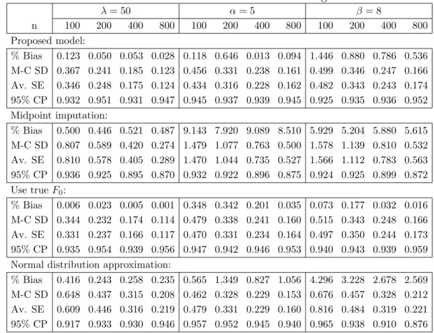
Table 4.1: Simulation result for wider censoring intervals.
λ= 50 α= 5 β = 8 n 100 200 400 800 100 200 400 800 100 200 400 800 Proposed model: % Bias 0.182 0.052 0.047 0.017 0.117 0.464 0.115 0.189 0.417 0.212 0.240 0.178 M-C SD 0.453 0.291 0.215 0.147 0.254 0.173 0.128 0.086 0.278 0.193 0.137 0.094 Av. SE 0.425 0.297 0.207 0.146 0.244 0.175 0.124 0.088 0.274 0.192 0.134 0.096 95% CP 0.916 0.944 0.937 0.945 0.939 0.938 0.942 0.948 0.942 0.949 0.939 0.951 Midpoint imputation: % Bias 1.195 1.135 1.223 1.160 11.02 10.51 11.03 10.59 7.237 7.005 7.217 7.035 M-C SD 1.041 0.748 0.530 0.360 1.023 0.710 0.508 0.350 1.139 0.774 0.556 0.388 Av. SE 1.031 0.738 0.521 0.371 0.987 0.710 0.504 0.359 1.086 0.782 0.556 0.396 95% CP 0.915 0.870 0.789 0.655 0.907 0.879 0.804 0.682 0.904 0.883 0.818 0.699 Use trueF0: % Bias 0.018 0.022 0.006 0.006 0.226 0.121 0.130 0.028 0.013 0.114 0.015 0.006 M-C SD 0.354 0.245 0.177 0.119 0.257 0.176 0.126 0.085 0.277 0.190 0.134 0.092 Av. SE 0.343 0.245 0.172 0.121 0.252 0.178 0.125 0.087 0.269 0.190 0.132 0.094 95% CP 0.947 0.948 0.932 0.944 0.948 0.947 0.944 0.953 0.940 0.949 0.933 0.957 Normal distribution approximation:
% Bias 0.463 0.255 0.245 0.223 0.170 0.361 0.167 0.345 1.723 1.267 0.978 0.910 M-C SD 0.792 0.568 0.398 0.269 0.261 0.184 0.129 0.088 0.342 0.238 0.169 0.112 Av. SE 0.738 0.555 0.394 0.278 0.257 0.183 0.129 0.090 0.380 0.251 0.172 0.120 95% CP 0.912 0.926 0.941 0.942 0.942 0.944 0.945 0.957 0.964 0.951 0.931 0.930
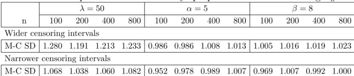
A second set of simulation was conducted to assess the influence of interval width on the performance of the estimation. We used the same simulation scheme as in the first set of simulation, but generated a series of the assessment times uniformly from non-overlapping intervals (j, j+ 1],j = 0,1, . . . .The resulted censoring intervals were narrower than that in the first set of simulation. The simulation results were summarized in Table 4.2.
Tables 4.1 and 4.2 show that the estimation bias is virtually ignorable in the proposed method, even with a moderate sample size (n = 100). The average bootstrap