Independent Component Analysis:
Algorithms and Applications
Aapo Hyvärinen and Erkki Oja
Neural Networks Research Centre
Helsinki University of Technology
P.O. Box 5400, FIN-02015 HUT, Finland
Neural Networks, 13(4-5):411-430, 2000
Abstract
A fundamental problem in neural network research, as well as in many other disciplines, is finding a suitable representation of multivariate data, i.e. random vectors. For reasons of computational and conceptual simplicity, the representation is often sought as a linear transformation of the original data. In other words, each component of the representation is a linear combination of the original variables. Well-known linear transformation methods include principal component analysis, factor analysis, and projection pursuit. Independent component analysis (ICA) is a recently developed method in which the goal is to find a linear representation of nongaussian data so that the components are statistically independent, or as independent as possible. Such a representation seems to capture the essential structure of the data in many applications, including feature extraction and signal separation. In this paper, we present the basic theory and applications of ICA, and our recent work on the subject.
Keywords: Independent component analysis, projection pursuit, blind signal separation, source separation, factor analysis, representation
1
Motivation
Imagine that you are in a room where two people are speaking simultaneously. You have two microphones, which you hold in different locations. The microphones give you two recorded time signals, which we could denote by
x1(t)and x2(t), with x1and x2the amplitudes, and t the time index. Each of these recorded signals is a weighted
sum of the speech signals emitted by the two speakers, which we denote by s1(t)and s2(t). We could express this
as a linear equation:
x1(t) =a11s1+a12s2 (1)
x2(t) =a21s1+a22s2 (2)
where a11,a12,a21, and a22are some parameters that depend on the distances of the microphones from the speakers.
It would be very useful if you could now estimate the two original speech signals s1(t)and s2(t), using only the
recorded signals x1(t)and x2(t). This is called the cocktail-party problem. For the time being, we omit any time
delays or other extra factors from our simplified mixing model.
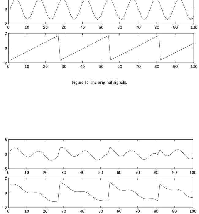
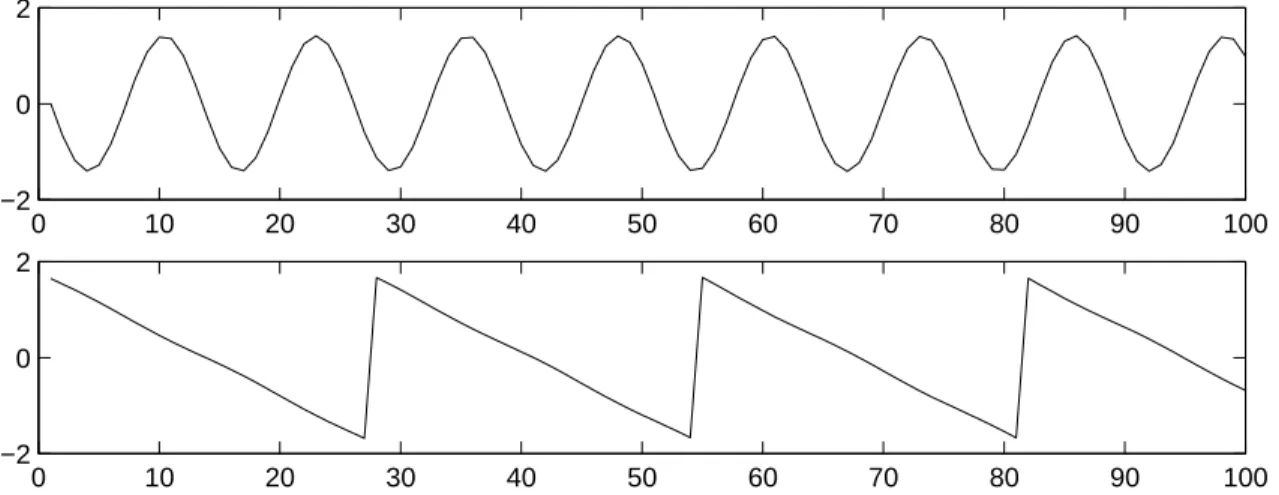
As an illustration, consider the waveforms in Fig. 1 and Fig. 2. These are, of course, not realistic speech signals, but suffice for this illustration. The original speech signals could look something like those in Fig. 1 and the mixed signals could look like those in Fig. 2. The problem is to recover the data in Fig. 1 using only the data in Fig. 2.
Actually, if we knew the parameters ai j, we could solve the linear equation in (1) by classical methods. The
point is, however, that if you don’t know the ai j, the problem is considerably more difficult.
One approach to solving this problem would be to use some information on the statistical properties of the signals si(t)to estimate the aii. Actually, and perhaps surprisingly, it turns out that it is enough to assume that s1(t)
and it need not be exactly true in practice. The recently developed technique of Independent Component Analysis, or ICA, can be used to estimate the ai jbased on the information of their independence, which allows us to separate
the two original source signals s1(t)and s2(t)from their mixtures x1(t)and x2(t). Fig. 3 gives the two signals
estimated by the ICA method. As can be seen, these are very close to the original source signals (their signs are reversed, but this has no significance.)
Independent component analysis was originally developed to deal with problems that are closely related to the cocktail-party problem. Since the recent increase of interest in ICA, it has become clear that this principle has a lot of other interesting applications as well.
Consider, for example, electrical recordings of brain activity as given by an electroencephalogram (EEG). The EEG data consists of recordings of electrical potentials in many different locations on the scalp. These potentials are presumably generated by mixing some underlying components of brain activity. This situation is quite similar to the cocktail-party problem: we would like to find the original components of brain activity, but we can only observe mixtures of the components. ICA can reveal interesting information on brain activity by giving access to its independent components.
Another, very different application of ICA is on feature extraction. A fundamental problem in digital signal processing is to find suitable representations for image, audio or other kind of data for tasks like compression and denoising. Data representations are often based on (discrete) linear transformations. Standard linear transforma-tions widely used in image processing are the Fourier, Haar, cosine transforms etc. Each of them has its own favorable properties (Gonzales and Wintz, 1987).
It would be most useful to estimate the linear transformation from the data itself, in which case the transform could be ideally adapted to the kind of data that is being processed. Figure 4 shows the basis functions obtained by ICA from patches of natural images. Each image window in the set of training images would be a superposition of these windows so that the coefficient in the superposition are independent. Feature extraction by ICA will be explained in more detail later on.
All of the applications described above can actually be formulated in a unified mathematical framework, that of ICA. This is a very general-purpose method of signal processing and data analysis.
In this review, we cover the definition and underlying principles of ICA in Sections 2 and 3. Then, starting from Section 4, the ICA problem is solved on the basis of minimizing or maximizing certain conrast functions; this transforms the ICA problem to a numerical optimization problem. Many contrast functions are given and the relations between them are clarified. Section 5 covers a useful preprocessing that greatly helps solving the ICA problem, and Section 6 reviews one of the most efficient practical learning rules for solving the problem, the FastICA algorithm. Then, in Section 7, typical applications of ICA are covered: removing artefacts from brain signal recordings, finding hidden factors in financial time series, and reducing noise in natural images. Section 8 concludes the text.
2
Independent Component Analysis
2.1
Definition of ICA
To rigorously define ICA (Jutten and Hérault, 1991; Comon, 1994), we can use a statistical “latent variables” model. Assume that we observe n linear mixtures x1, ...,xnof n independent components
xj=aj1s1+aj2s2+...+ajnsn, for all j. (3)
We have now dropped the time index t; in the ICA model, we assume that each mixture xj as well as each
independent component skis a random variable, instead of a proper time signal. The observed values xj(t), e.g.,
the microphone signals in the cocktail party problem, are then a sample of this random variable. Without loss of generality, we can assume that both the mixture variables and the independent components have zero mean: If this is not true, then the observable variables xican always be centered by subtracting the sample mean, which makes
the model zero-mean.
It is convenient to use vector-matrix notation instead of the sums like in the previous equation. Let us denote by x the random vector whose elements are the mixtures x1, ...,xn, and likewise by s the random vector with elements
s1, ...,sn. Let us denote by A the matrix with elements ai j. Generally, bold lower case letters indicate vectors and
bold upper-case letters denote matrices. All vectors are understood as column vectors; thus xT, or the transpose of x, is a row vector. Using this vector-matrix notation, the above mixing model is written as
x=As. (4)
Sometimes we need the columns of matrix A; denoting them by ajthe model can also be written as
x=
n
∑
i=1
aisi. (5)
The statistical model in Eq. 4 is called independent component analysis, or ICA model. The ICA model is a generative model, which means that it describes how the observed data are generated by a process of mixing the components si. The independent components are latent variables, meaning that they cannot be directly observed.
Also the mixing matrix is assumed to be unknown. All we observe is the random vector x, and we must estimate both A and s using it. This must be done under as general assumptions as possible.
The starting point for ICA is the very simple assumption that the components siare statistically independent.
Statistical independence will be rigorously defined in Section 3. It will be seen below that we must also assume that the independent component must have nongaussian distributions. However, in the basic model we do not assume these distributions known (if they are known, the problem is considerably simplified.) For simplicity, we are also assuming that the unknown mixing matrix is square, but this assumption can be sometimes relaxed, as explained in Section 4.5. Then, after estimating the matrix A, we can compute its inverse, say W, and obtain the independent component simply by:
s=Wx. (6)
ICA is very closely related to the method called blind source separation (BSS) or blind signal separation. A “source” means here an original signal, i.e. independent component, like the speaker in a cocktail party problem. “Blind” means that we no very little, if anything, on the mixing matrix, and make little assumptions on the source signals. ICA is one method, perhaps the most widely used, for performing blind source separation.
In many applications, it would be more realistic to assume that there is some noise in the measurements (see e.g. (Hyvärinen, 1998a; Hyvärinen, 1999c)), which would mean adding a noise term in the model. For simplicity, we omit any noise terms, since the estimation of the noise-free model is difficult enough in itself, and seems to be sufficient for many applications.
2.2
Ambiguities of ICA
In the ICA model in Eq. (4), it is easy to see that the following ambiguities will hold: 1. We cannot determine the variances (energies) of the independent components.
The reason is that, both s and A being unknown, any scalar multiplier in one of the sources sicould always
be cancelled by dividing the corresponding column aiof A by the same scalar; see eq. (5). As a consequence,
we may quite as well fix the magnitudes of the independent components; as they are random variables, the most natural way to do this is to assume that each has unit variance: E{s2i}=1. Then the matrix A will be adapted in the ICA solution methods to take into account this restriction. Note that this still leaves the ambiguity of the sign: we could multiply the an independent component by−1 without affecting the model. This ambiguity is, fortunately, insignificant in most applications.
2. We cannot determine the order of the independent components.
The reason is that, again both s and A being unknown, we can freely change the order of the terms in the sum in (5), and call any of the independent components the first one. Formally, a permutation matrix P and its inverse can be substituted in the model to give x=AP−1Ps. The elements of Ps are the original independent variables sj,
2.3
Illustration of ICA
To illustrate the ICA model in statistical terms, consider two independent components that have the following uniform distributions: p(si) = ( 1 2√3 if|si| ≤ √ 3 0 otherwise (7)
The range of values for this uniform distribution were chosen so as to make the mean zero and the variance equal to one, as was agreed in the previous Section. The joint density of s1 and s2is then uniform on a square. This
follows from the basic definition that the joint density of two independent variables is just the product of their marginal densities (see Eq. 10): we need to simply compute the product. The joint density is illustrated in Figure 5 by showing data points randomly drawn from this distribution.
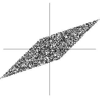
Now let as mix these two independent components. Let us take the following mixing matrix: A0= 2 3 2 1 (8) This gives us two mixed variables, x1and x2. It is easily computed that the mixed data has a uniform distribution
on a parallelogram, as shown in Figure 6. Note that the random variables x1and x2are not independent any more;
an easy way to see this is to consider, whether it is possible to predict the value of one of them, say x2, from the
value of the other. Clearly if x1attains one of its maximum or minimum values, then this completely determines
the value of x2. They are therefore not independent. (For variables s1and s2the situation is different: from Fig. 5
it can be seen that knowing the value of s1does not in any way help in guessing the value of s2.)
The problem of estimating the data model of ICA is now to estimate the mixing matrix A0using only
infor-mation contained in the mixtures x1and x2. Actually, you can see from Figure 6 an intuitive way of estimating A:
The edges of the parallelogram are in the directions of the columns of A. This means that we could, in principle, estimate the ICA model by first estimating the joint density of x1and x2, and then locating the edges. So, the
problem seems to have a solution.
In reality, however, this would be a very poor method because it only works with variables that have exactly uniform distributions. Moreover, it would be computationally quite complicated. What we need is a method that works for any distributions of the independent components, and works fast and reliably.
Next we shall consider the exact definition of independence before starting to develop methods for estimation of the ICA model.
3
What is independence?
3.1
Definition and fundamental properties
To define the concept of independence, consider two scalar-valued random variables y1 and y2. Basically, the
variables y1and y2are said to be independent if information on the value of y1does not give any information on
the value of y2, and vice versa. Above, we noted that this is the case with the variables s1,s2but not with the
mixture variables x1,x2.
Technically, independence can be defined by the probability densities. Let us denote by p(y1,y2)the joint
probability density function (pdf) of y1and y2. Let us further denote by p1(y1)the marginal pdf of y1, i.e. the pdf
of y1when it is considered alone:
p1(y1) =
Z
p(y1,y2)dy2, (9)
and similarly for y2. Then we define that y1and y2are independent if and only if the joint pdf is factorizable in the
following way:
p(y1,y2) =p1(y1)p2(y2). (10)
This definition extends naturally for any number n of random variables, in which case the joint density must be a product of n terms.
The definition can be used to derive a most important property of independent random variables. Given two functions, h1and h2, we always have
E{h1(y1)h2(y2)}=E{h1(y1)}E{h2(y2)}. (11)
This can be proven as follows:
E{h1(y1)h2(y2)}= Z Z h1(y1)h2(y2)p(y1,y2)dy1dy2 = Z Z h1(y1)p1(y1)h2(y2)p2(y2)dy1dy2= Z h1(y1)p1(y1)dy1 Z h2(y2)p2(y2)dy2 =E{h1(y1)}E{h2(y2)}. (12)
3.2
Uncorrelated variables are only partly independent
A weaker form of independence is uncorrelatedness. Two random variables y1and y2are said to be uncorrelated,
if their covariance is zero:
E{y1y2} −E{y1}E{y2}=0 (13)
If the variables are independent, they are uncorrelated, which follows directly from Eq. (11), taking h1(y1) =y1
and h2(y2) =y2.
On the other hand, uncorrelatedness does not imply independence. For example, assume that(y1,y2)are
discrete valued and follow such a distribution that the pair are with probability 1/4 equal to any of the following values: (0,1),(0,−1),(1,0),(−1,0). Then y1and y2are uncorrelated, as can be simply calculated. On the other
hand,
E{y21y22}=06=1
4=E{y
2
1}E{y22}. (14)
so the condition in Eq. (11) is violated, and the variables cannot be independent.
Since independence implies uncorrelatedness, many ICA methods constrain the estimation procedure so that it always gives uncorrelated estimates of the independent components. This reduces the number of free parameters, and simplifies the problem.
3.3
Why Gaussian variables are forbidden
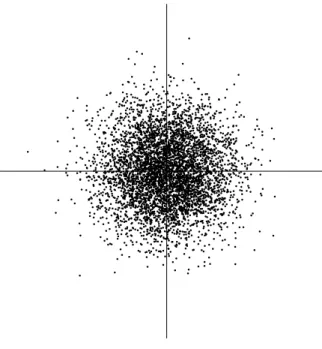
The fundamental restriction in ICA is that the independent components must be nongaussian for ICA to be possible. To see why gaussian variables make ICA impossible, assume that the mixing matrix is orthogonal and the si
are gaussian. Then x1and x2are gaussian, uncorrelated, and of unit variance. Their joint density is given by
p(x1,x2) = 1
2πexp(−
x21+x22
2 ) (15)
This distribution is illustrated in Fig. 7. The Figure shows that the density is completely symmetric. Therefore, it does not contain any information on the directions of the columns of the mixing matrix A. This is why A cannot be estimated.
More rigorously, one can prove that the distribution of any orthogonal transformation of the gaussian(x1,x2)
has exactly the same distribution as(x1,x2), and that x1and x2 are independent. Thus, in the case of gaussian
variables, we can only estimate the ICA model up to an orthogonal transformation. In other words, the matrix A is not identifiable for gaussian independent components. (Actually, if just one of the independent components is gaussian, the ICA model can still be estimated.)
4
Principles of ICA estimation
4.1
“Nongaussian is independent”
Intuitively speaking, the key to estimating the ICA model is nongaussianity. Actually, without nongaussianity the estimation is not possible at all, as mentioned in Sec. 3.3. This is at the same time probably the main reason for the rather late resurgence of ICA research: In most of classical statistical theory, random variables are assumed to have gaussian distributions, thus precluding any methods related to ICA.
The Central Limit Theorem, a classical result in probability theory, tells that the distribution of a sum of independent random variables tends toward a gaussian distribution, under certain conditions. Thus, a sum of two independent random variables usually has a distribution that is closer to gaussian than any of the two original random variables.
Let us now assume that the data vector x is distributed according to the ICA data model in Eq. 4, i.e. it is a mixture of independent components. For simplicity, let us assume in this section that all the independent components have identical distributions. To estimate one of the independent components, we consider a linear combination of the xi(see eq. 6); let us denote this by y=wTx=∑iwixi, where w is a vector to be determined. If
w were one of the rows of the inverse of A, this linear combination would actually equal one of the independent components. The question is now: How could we use the Central Limit Theorem to determine w so that it would equal one of the rows of the inverse of A? In practice, we cannot determine such a w exactly, because we have no knowledge of matrix A, but we can find an estimator that gives a good approximation.
To see how this leads to the basic principle of ICA estimation, let us make a change of variables, defining z=ATw. Then we have y=wTx=wTAs=zTs. y is thus a linear combination of si, with weights given by zi.
Since a sum of even two independent random variables is more gaussian than the original variables, zTs is more gaussian than any of the siand becomes least gaussian when it in fact equals one of the si. In this case, obviously
only one of the elements ziof z is nonzero. (Note that the siwere here assumed to have identical distributions.)
Therefore, we could take as w a vector that maximizes the nongaussianity of wTx. Such a vector would necessarily correspond (in the transformed coordinate system) to a z which has only one nonzero component. This means that wTx=zTs equals one of the independent components!
Maximizing the nongaussianity of wTx thus gives us one of the independent components. In fact, the
opti-mization landscape for nongaussianity in the n-dimensional space of vectors w has 2n local maxima, two for each independent component, corresponding to si and−si (recall that the independent components can be estimated
only up to a multiplicative sign). To find several independent components, we need to find all these local maxima. This is not difficult, because the different independent components are uncorrelated: We can always constrain the search to the space that gives estimates uncorrelated with the previous ones. This corresponds to orthogonalization in a suitably transformed (i.e. whitened) space.
Our approach here is rather heuristic, but it will be seen in the next section and Sec. 4.3 that it has a perfectly rigorous justification.
4.2
Measures of nongaussianity
To use nongaussianity in ICA estimation, we must have a quantitative measure of nongaussianity of a random variable, say y. To simplify things, let us assume that y is centered (zero-mean) and has variance equal to one. Actually, one of the functions of preprocessing in ICA algorithms, to be covered in Section 5, is to make this simplification possible.
4.2.1 Kurtosis
The classical measure of nongaussianity is kurtosis or the fourth-order cumulant. The kurtosis of y is classically defined by
kurt(y) =E{y4} −3(E{y2})2 (16)
Actually, since we assumed that y is of unit variance, the right-hand side simplifies to E{y4} −3. This shows that kurtosis is simply a normalized version of the fourth moment E{y4}. For a gaussian y, the fourth moment equals
3(E{y2})2. Thus, kurtosis is zero for a gaussian random variable. For most (but not quite all) nongaussian random
variables, kurtosis is nonzero.
Kurtosis can be both positive or negative. Random variables that have a negative kurtosis are called sub-gaussian, and those with positive kurtosis are called supergaussian. In statistical literature, the corresponding expressions platykurtic and leptokurtic are also used. Supergaussian random variables have typically a “spiky” pdf with heavy tails, i.e. the pdf is relatively large at zero and at large values of the variable, while being small for intermediate values. A typical example is the Laplace distribution, whose pdf (normalized to unit variance) is given by
p(y) =√1
2exp(
√
2|y|) (17)
This pdf is illustrated in Fig. 8. Subgaussian random variables, on the other hand, have typically a “flat” pdf, which is rather constant near zero, and very small for larger values of the variable. A typical example is the uniform distibution in eq. (7).
Typically nongaussianity is measured by the absolute value of kurtosis. The square of kurtosis can also be used. These are zero for a gaussian variable, and greater than zero for most nongaussian random variables. There are nongaussian random variables that have zero kurtosis, but they can be considered as very rare.
Kurtosis, or rather its absolute value, has been widely used as a measure of nongaussianity in ICA and related fields. The main reason is its simplicity, both computational and theoretical. Computationally, kurtosis can be estimated simply by using the fourth moment of the sample data. Theoretical analysis is simplified because of the following linearity property: If x1and x2are two independent random variables, it holds
kurt(x1+x2) =kurt(x1) +kurt(x2) (18)
and
kurt(αx1) =α4kurt(x1) (19) whereαis a scalar. These properties can be easily proven using the definition.
To illustrate in a simple example what the optimization landscape for kurtosis looks like, and how independent components could be found by kurtosis minimization or maximization, let us look at a 2-dimensional model x=
As. Assume that the independent components s1,s2 have kurtosis values kurt(s1),kurt(s2), respectively, both
different from zero. Remember that we assumed that they have unit variances. We seek for one of the independent components as y=wTx.
Let us again make the transformation z=ATw. Then we have y=wTx=wTAs=zTs=z
1s1+z2s2. Now,
based on the additive property of kurtosis, we have kurt(y) = kurt(z1s1) +kurt(z2s2) =z41kurt(s1) +z42kurt(s2).
On the other hand, we made the constraint that the variance of y is equal to 1, based on the same assumption concerning s1,s2. This implies a constraint on z: E{y2}=z21+z22=1. Geometrically, this means that vector z is
constrained to the unit circle on the 2-dimensional plane. The optimization problem is now: what are the maxima of the function|kurt(y)|=|z41kurt(s1) +z42kurt(s2)|on the unit circle? For simplicity, you may consider that the
kurtosis are of the same sign, in which case it absolute value operators can be omitted. The graph of this function is the "optimization landscape" for the problem.
It is not hard to show (Delfosse and Loubaton, 1995) that the maxima are at the points when exactly one of the elements of vector z is zero and the other nonzero; because of the unit circle constraint, the nonzero element must be equal to 1 or -1. But these points are exactly the ones when y equals one of the independent components±si,
and the problem has been solved.
In practice we would start from some weight vector w, compute the direction in which the kurtosis of y=wTx is growing most strongly (if kurtosis is positive) or decreasing most strongly (if kurtosis is negative) based on the available sample x(1), ...,x(T)of mixture vector x, and use a gradient method or one of their extensions for finding a new vector w. The example can be generalized to arbitrary dimensions, showing that kurtosis can theoretically be used as an optimization criterion for the ICA problem.
However, kurtosis has also some drawbacks in practice, when its value has to be estimated from a measured sample. The main problem is that kurtosis can be very sensitive to outliers (Huber, 1985). Its value may depend on only a few observations in the tails of the distribution, which may be erroneous or irrelevant observations. In other words, kurtosis is not a robust measure of nongaussianity.
Thus, other measures of nongaussianity might be better than kurtosis in some situations. Below we shall consider negentropy whose properties are rather opposite to those of kurtosis, and finally introduce approximations of negentropy that more or less combine the good properties of both measures.
4.2.2 Negentropy
A second very important measure of nongaussianity is given by negentropy. Negentropy is based on the information-theoretic quantity of (differential) entropy.
Entropy is the basic concept of information theory. The entropy of a random variable can be interpreted as the degree of information that the observation of the variable gives. The more “random”, i.e. unpredictable and unstructured the variable is, the larger its entropy. More rigorously, entropy is closely related to the coding length of the random variable, in fact, under some simplifying assumptions, entropy is the coding length of the random variable. For introductions on information theory, see e.g. (Cover and Thomas, 1991; Papoulis, 1991).
Entropy H is defined for a discrete random variable Y as
H(Y) =−
∑
i
P(Y =ai)log P(Y =ai) (20)
where the aiare the possible values of Y . This very well-known definition can be generalized for continuous-valued
random variables and vectors, in which case it is often called differential entropy. The differential entropy H of a random vector y with density f(y)is defined as (Cover and Thomas, 1991; Papoulis, 1991):
H(y) =−
Z
f(y)log f(y)dy. (21) A fundamental result of information theory is that a gaussian variable has the largest entropy among all
random variables of equal variance. For a proof, see e.g. (Cover and Thomas, 1991; Papoulis, 1991). This means
that entropy could be used as a measure of nongaussianity. In fact, this shows that the gaussian distribution is the “most random” or the least structured of all distributions. Entropy is small for distributions that are clearly concentrated on certain values, i.e., when the variable is clearly clustered, or has a pdf that is very “spiky”.
To obtain a measure of nongaussianity that is zero for a gaussian variable and always nonnegative, one often uses a slightly modified version of the definition of differential entropy, called negentropy. Negentropy J is defined as follows
J(y) =H(ygauss)−H(y) (22)
where ygauss is a Gaussian random variable of the same covariance matrix as y. Due to the above-mentioned
properties, negentropy is always non-negative, and it is zero if and only if y has a Gaussian distribution. Negen-tropy has the additional interesting property that it is invariant for invertible linear transformations (Comon, 1994; Hyvärinen, 1999e).
The advantage of using negentropy, or, equivalently, differential entropy, as a measure of nongaussianity is that it is well justified by statistical theory. In fact, negentropy is in some sense the optimal estimator of nongaussianity, as far as statistical properties are concerned. The problem in using negentropy is, however, that it is computationally very difficult. Estimating negentropy using the definition would require an estimate (possibly nonparametric) of the pdf. Therefore, simpler approximations of negentropy are very useful, as will be discussed next.
4.2.3 Approximations of negentropy
The estimation of negentropy is difficult, as mentioned above, and therefore this contrast function remains mainly a theoretical one. In practice, some approximation have to be used. Here we introduce approximations that have very promising properties, and which will be used in the following to derive an efficient method for ICA.
The classical method of approximating negentropy is using higher-order moments, for example as follows (Jones and Sibson, 1987):
J(y)≈121 E{y3}2+ 1
48kurt(y)
The random variable y is assumed to be of zero mean and unit variance. However, the validity of such approxima-tions may be rather limited. In particular, these approximaapproxima-tions suffer from the nonrobustness encountered with kurtosis.
To avoid the problems encountered with the preceding approximations of negentropy, new approximations were developed in (Hyvärinen, 1998b). These approximation were based on the maximum-entropy principle. In general we obtain the following approximation:
J(y)≈
p
∑
i=1
ki[E{Gi(y)} −E{Gi(ν)}]2, (24)
where kiare some positive constants, andνis a Gaussian variable of zero mean and unit variance (i.e.,
standard-ized). The variable y is assumed to be of zero mean and unit variance, and the functions Giare some nonquadratic
functions (Hyvärinen, 1998b). Note that even in cases where this approximation is not very accurate, (24) can be used to construct a measure of nongaussianity that is consistent in the sense that it is always non-negative, and equal to zero if y has a Gaussian distribution.
In the case where we use only one nonquadratic function G, the approximation becomes
J(y)∝[E{G(y)} −E{G(ν)}]2 (25)
for practically any non-quadratic function G. This is clearly a generalization of the moment-based approximation in (23), if y is symmetric. Indeed, taking G(y) =y4, one then obtains exactly (23), i.e. a kurtosis-based approximation. But the point here is that by choosing G wisely, one obtains approximations of negentropy that are much better than the one given by (23). In particular, choosing G that does not grow too fast, one obtains more robust estimators. The following choices of G have proved very useful:
G1(u) =
1
a1
log cosh a1u, G2(u) =−exp(−u2/2) (26)
where 1≤a1≤2 is some suitable constant.
Thus we obtain approximations of negentropy that give a very good compromise between the properties of the two classical nongaussianity measures given by kurtosis and negentropy. They are conceptually simple, fast to compute, yet have appealing statistical properties, especially robustness. Therefore, we shall use these contrast functions in our ICA methods. Since kurtosis can be expressed in this same framework, it can still be used by our ICA methods. A practical algorithm based on these contrast function will be presented in Section 6.
4.3
Minimization of Mutual Information
Another approach for ICA estimation, inspired by information theory, is minimization of mutual information. We will explain this approach here, and show that it leads to the same principle of finding most nongaussian directions as was described above. In particular, this approach gives a rigorous justification for the heuristic principles used above.
4.3.1 Mutual Information
Using the concept of differential entropy, we define the mutual information I between m (scalar) random variables,
yi,i=1...m as follows I(y1,y2, ...,ym) = m
∑
i=1 H(yi)−H(y). (27)Mutual information is a natural measure of the dependence between random variables. In fact, it is equivalent to the well-known Kullback-Leibler divergence between the joint density f(y) and the product of its marginal densities; a very natural measure for independence. It is always non-negative, and zero if and only if the variables are statistically independent. Thus, mutual information takes into account the whole dependence structure of the variables, and not only the covariance, like PCA and related methods.
Mutual information can be interpreted by using the interpretation of entropy as code length. The terms H(yi)
give the lengths of codes for the yi when these are coded separately, and H(y)gives the code length when y is
coded as a random vector, i.e. all the components are coded in the same code. Mutual information thus shows what code length reduction is obtained by coding the whole vector instead of the separate components. In general, better codes can be obtained by coding the whole vector. However, if the yiare independent, they give no information on
each other, and one could just as well code the variables separately without increasing code length.
An important property of mutual information (Papoulis, 1991; Cover and Thomas, 1991) is that we have for an invertible linear transformation y=Wx:
I(y1,y2, ...,yn) =
∑
iH(yi)−H(x)−log|det W|. (28)
Now, let us consider what happens if we constrain the yi to be uncorrelated and of unit variance. This means
E{yyT}=WE{xxT}WT =I, which implies
det I=1= (det WE{xxT}WT) = (det W)(det E{xxT})(det WT), (29) and this implies that det W must be constant. Moreover, for yiof unit variance, entropy and negentropy differ only
by a constant, and the sign. Thus we obtain,
I(y1,y2, ...,yn) =C−
∑
iJ(yi). (30)
where C is a constant that does not depend on W. This shows the fundamental relation between negentropy and mutual information.
4.3.2 Defining ICA by Mutual Information
Since mutual information is the natural information-theoretic measure of the independence of random variables, we could use it as the criterion for finding the ICA transform. In this approach that is an alternative to the model estimation approach, we define the ICA of a random vector x as an invertible transformation as in (6), where the matrix W is determined so that the mutual information of the transformed components siis minimized.
It is now obvious from (30) that finding an invertible transformation W that minimizes the mutual information is roughly equivalent to finding directions in which the negentropy is maximized. More precisely, it is roughly equiva-lent to finding 1-D subspaces such that the projections in those subspaces have maximum negentropy. Rigorously, speaking, (30) shows that ICA estimation by minimization of mutual information is equivalent to maximizing the sum of nongaussianities of the estimates, when the estimates are constrained to be uncorrelated. The constraint of uncorrelatedness is in fact not necessary, but simplifies the computations considerably, as one can then use the simpler form in (30) instead of the more complicated form in (28).
Thus, we see that the formulation of ICA as minimization of mutual information gives another rigorous justi-fication of our more heuristically introduced idea of finding maximally nongaussian directions.
4.4
Maximum Likelihood Estimation
4.4.1 The likelihood
A very popular approach for estimating the ICA model is maximum likelihood estimation, which is closely con-nected to the infomax principle. Here we discuss this approach, and show that it is essentially equivalent to minimization of mutual information.
It is possible to formulate directly the likelihood in the noise-free ICA model, which was done in (Pham et al., 1992), and then estimate the model by a maximum likelihood method. Denoting by W= (w1, ...,wn)T the matrix
A−1, the log-likelihood takes the form (Pham et al., 1992):
L= T
∑
t=1 n∑
i=1where the fi are the density functions of the si (here assumed to be known), and the x(t),t =1, ...,T are the
realizations of x. The term log|det W|in the likelihood comes from the classic rule for (linearly) transforming random variables and their densities (Papoulis, 1991): In general, for any random vector x with density pxand for
any matrix W, the density of y=Wx is given by px(Wx)|det W|.
4.4.2 The Infomax Principle
Another related contrast function was derived from a neural network viewpoint in (Bell and Sejnowski, 1995; Nadal and Parga, 1994). This was based on maximizing the output entropy (or information flow) of a neural network with non-linear outputs. Assume that x is the input to the neural network whose outputs are of the form
φi(wTi x), where theφiare some non-linear scalar functions, and the wiare the weight vectors of the neurons. One
then wants to maximize the entropy of the outputs:
L2=H(φ1(wT1x), ...,φn(wTnx)). (32)
If theφiare well chosen, this framework also enables the estimation of the ICA model. Indeed, several authors, e.g.,
(Cardoso, 1997; Pearlmutter and Parra, 1997), proved the surprising result that the principle of network entropy maximization, or “infomax”, is equivalent to maximum likelihood estimation. This equivalence requires that the non-linearitiesφiused in the neural network are chosen as the cumulative distribution functions corresponding to
the densities fi, i.e.,φ0i(.) = fi(.).
4.4.3 Connection to mutual information
To see the connection between likelihood and mutual information, consider the expectation of the log-likelihood: 1
TE{L}=
n
∑
i=1
E{log fi(wTix)}+log|det W|. (33)
Actually, if the fi were equal to the actual distributions of wTix, the first term would be equal to−∑iH(wTix).
Thus the likelihood would be equal, up to an additive constant, to the negative of mutual information as given in Eq. (28).
Actually, in practice the connection is even stronger. This is because in practice we don’t know the distributions of the independent components. A reasonable approach would be to estimate the density of wTix as part of the ML estimation method, and use this as an approximation of the density of si. In this case, likelihood and mutual
information are, for all practical purposes, equivalent.
Nevertheless, there is a small difference that may be very important in practice. The problem with maximum likelihood estimation is that the densities fi must be estimated correctly. They need not be estimated with any
great precision: in fact it is enough to estimate whether they are sub- or supergaussian (Cardoso and Laheld, 1996; Hyvärinen and Oja, 1998; Lee et al., 1999). In many cases, in fact, we have enough prior knowledge on the independent components, and we don’t need to estimate their nature from the data. In any case, if the information on the nature of the independent components is not correct, ML estimation will give completely wrong results. Some care must be taken with ML estimation, therefore. In contrast, using reasonable measures of nongaussianity, this problem does not usually arise.
4.5
ICA and Projection Pursuit
It is interesting to note how our approach to ICA makes explicit the connection between ICA and projection pursuit. Projection pursuit (Friedman and Tukey, 1974; Friedman, 1987; Huber, 1985; Jones and Sibson, 1987) is a technique developed in statistics for finding “interesting” projections of multidimensional data. Such projections can then be used for optimal visualization of the data, and for such purposes as density estimation and regression. In basic (1-D) projection pursuit, we try to find directions such that the projections of the data in those directions have interesting distributions, i.e., display some structure. It has been argued by Huber (Huber, 1985) and by Jones and Sibson (Jones and Sibson, 1987) that the Gaussian distribution is the least interesting one, and that the most
interesting directions are those that show the least Gaussian distribution. This is exactly what we do to estimate the ICA model.
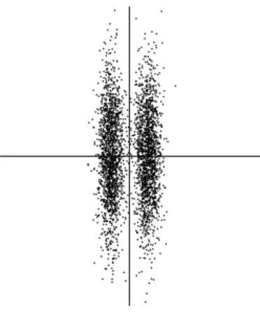
The usefulness of finding such projections can be seen in Fig. 9, where the projection on the projection pursuit direction, which is horizontal, clearly shows the clustered structure of the data. The projection on the first principal component (vertical), on the other hand, fails to show this structure.
Thus, in the general formulation, ICA can be considered a variant of projection pursuit. All the nongaussianity measures and the corresponding ICA algorithms presented here could also be called projection pursuit “indices” and algorithms. In particular, the projection pursuit allows us to tackle the situation where there are less indepen-dent components sithan original variables xiis. Assuming that those dimensions of the space that are not spanned
by the independent components are filled by gaussian noise, we see that computing the nongaussian projection pursuit directions, we effectively estimate the independent components. When all the nongaussian directions have been found, all the independent components have been estimated. Such a procedure can be interpreted as a hybrid of projection pursuit and ICA.
However, it should be noted that in the formulation of projection pursuit, no data model or assumption about independent components is made. If the ICA model holds, optimizing the ICA nongaussianity measures produce independent components; if the model does not hold, then what we get are the projection pursuit directions.
5
Preprocessing for ICA
In the preceding section, we discussed the statistical principles underlying ICA methods. Practical algorithms based on these principles will be discussed in the next section. However, before applying an ICA algorithm on the data, it is usually very useful to do some preprocessing. In this section, we discuss some preprocessing techniques that make the problem of ICA estimation simpler and better conditioned.
5.1
Centering
The most basic and necessary preprocessing is to center x, i.e. subtract its mean vector m=E{x}so as to make x a zero-mean variable. This implies that s is zero-mean as well, as can be seen by taking expectations on both sides of Eq. (4).
This preprocessing is made solely to simplify the ICA algorithms: It does not mean that the mean could not be estimated. After estimating the mixing matrix A with centered data, we can complete the estimation by adding the mean vector of s back to the centered estimates of s. The mean vector of s is given by A−1m, where m is the mean that was subtracted in the preprocessing.
5.2
Whitening
Another useful preprocessing strategy in ICA is to first whiten the observed variables. This means that before the application of the ICA algorithm (and after centering), we transform the observed vector x linearly so that we obtain a new vector ˜x which is white, i.e. its components are uncorrelated and their variances equal unity. In other words, the covariance matrix of ˜x equals the identity matrix:
E{˜x˜xT}=I. (34)
The whitening transformation is always possible. One popular method for whitening is to use the eigen-value decomposition (EVD) of the covariance matrix E{xxT}=EDET, where E is the orthogonal matrix of eigenvectors of E{xxT}and D is the diagonal matrix of its eigenvalues, D=diag(d1, ...,dn). Note that E{xxT}can be estimated
in a standard way from the available sample x(1), ...,x(T). Whitening can now be done by
˜x=ED−1/2ETx (35)
where the matrix D−1/2is computed by a simple component-wise operation as D−1/2=diag(d1−1/2, ...,d−n1/2). It
Whitening transforms the mixing matrix into a new one, ˜A. We have from (4) and (35):
˜x=ED−1/2ETAs=As˜ (36)
The utility of whitening resides in the fact that the new mixing matrix ˜A is orthogonal. This can be seen from
E{˜x˜xT}=AE˜ {ssT}A˜T=A ˜˜AT=I. (37)
Here we see that whitening reduces the number of parameters to be estimated. Instead of having to estimate the
n2parameters that are the elements of the original matrix A, we only need to estimate the new, orthogonal mixing matrix ˜A. An orthogonal matrix contains n(n−1)/2 degrees of freedom. For example, in two dimensions, an orthogonal transformation is determined by a single angle parameter. In larger dimensions, an orthogonal matrix contains only about half of the number of parameters of an arbitrary matrix. Thus one can say that whitening solves half of the problem of ICA. Because whitening is a very simple and standard procedure, much simpler than any ICA algorithms, it is a good idea to reduce the complexity of the problem this way.
It may also be quite useful to reduce the dimension of the data at the same time as we do the whitening. Then we look at the eigenvalues dj of E{xxT} and discard those that are too small, as is often done in the statistical
technique of principal component analysis. This has often the effect of reducing noise. Moreover, dimension reduction prevents overlearning, which can sometimes be observed in ICA (Hyvärinen et al., 1999).
A graphical illustration of the effect of whitening can be seen in Figure 10, in which the data in Figure 6 has been whitened. The square defining the distribution is now clearly a rotated version of the original square in Figure 5. All that is left is the estimation of a single angle that gives the rotation.
In the rest of this paper, we assume that the data has been preprocessed by centering and whitening. For simplicity of notation, we denote the preprocessed data just by x, and the transformed mixing matrix by A, omitting the tildes.
5.3
Further preprocessing
The success of ICA for a given data set may depende crucially on performing some application-dependent prepro-cessing steps. For example, if the data consists of time-signals, some band-pass filtering may be very useful. Note that if we filter linearly the observed signals xi(t)to obtain new signals, say x∗i(t), the ICA model still holds for
x∗i(t), with the same mixing matrix.
This can be seen as follows. Denote by X the matrix that contains the observations x(1), ...,x(T)as its columns, and similarly for S. Then the ICA model can be expressed as:
X=AS (38)
Now, time filtering of X corresponds to multiplying X from the right by a matrix, let us call it M. This gives
X∗=XM=ASM=AS∗, (39)
which shows that the ICA model remains still valid.
6
The FastICA Algorithm
In the preceding sections, we introduced different measures of nongaussianity, i.e. objective functions for ICA estimation. In practice, one also needs an algorithm for maximizing the contrast function, for example the one in (25). In this section, we introduce a very efficient method of maximization suited for this task. It is here assumed that the data is preprocessed by centering and whitening as discussed in the preceding section.
6.1
FastICA for one unit
To begin with, we shall show the one-unit version of FastICA. By a "unit" we refer to a computational unit, eventually an artificial neuron, having a weight vector w that the neuron is able to update by a learning rule. The FastICA learning rule finds a direction, i.e. a unit vector w such that the projection wTx maximizes nongaussianity. Nongaussianity is here measured by the approximation of negentropy J(wTx)given in (25). Recall that the variance of wTx must here be constrained to unity; for whitened data this is equivalent to constraining the norm of w to be
unity.
The FastICA is based on a fixed-point iteration scheme for finding a maximum of the nongaussianity of wTx, as measured in (25), see (Hyvärinen and Oja, 1997; Hyvärinen, 1999a). It can be also derived as an approximative Newton iteration (Hyvärinen, 1999a). Denote by g the derivative of the nonquadratic function G used in (25); for example the derivatives of the functions in (26) are:
g1(u) =tanh(a1u), (40)
g2(u) =u exp(−u2/2)
where 1≤a1≤2 is some suitable constant, often taken as a1=1. The basic form of the FastICA algorithm is as
follows:
1. Choose an initial (e.g. random) weight vector w. 2. Let w+=E{xg(wTx)} −E{g0(wTx)}w 3. Let w=w+/kw+k
4. If not converged, go back to 2.
Note that convergence means that the old and new values of w point in the same direction, i.e. their dot-product is (almost) equal to 1. It is not necessary that the vector converges to a single point, since w and−w define the same direction. This is again because the independent components can be defined only up to a multiplicative sign. Note also that it is here assumed that the data is prewhitened.
The derivation of FastICA is as follows. First note that the maxima of the approximation of the negentropy of wTx are obtained at certain optima of E{G(wTx)}. According to the Kuhn-Tucker conditions (Luenberger, 1969), the optima of E{G(wTx)}under the constraint E{(wTx)2}=kwk2=1 are obtained at points where
E{xg(wTx)} −βw=0 (41)
Let us try to solve this equation by Newton’s method. Denoting the function on the left-hand side of (41) by F, we obtain its Jacobian matrix JF(w)as
JF(w) =E{xxTg0(wTx)} −βI (42)
To simplify the inversion of this matrix, we decide to approximate the first term in (42). Since the data is sphered, a reasonable approximation seems to be E{xxTg0(wTx)} ≈E{xxT}E{g0(wTx)}=E{g0(wTx)}I. Thus the Jaco-bian matrix becomes diagonal, and can easily be inverted. Thus we obtain the following approximative Newton iteration:
w+=w−[E{xg(wTx)} −βw]/[E{g0(wTx)} −β] (43) This algorithm can be further simplified by multiplying both sides of (43) byβ−E{g0(wTx)}. This gives, after algebraic simplication, the FastICA iteration.
In practice, the expectations in FastICA must be replaced by their estimates. The natural estimates are of course the corresponding sample means. Ideally, all the data available should be used, but this is often not a good idea because the computations may become too demanding. Then the averages can be estimated using a smaller sample, whose size may have a considerable effect on the accuracy of the final estimates. The sample points should be chosen separately at every iteration. If the convergence is not satisfactory, one may then increase the sample size.
6.2
FastICA for several units
The one-unit algorithm of the preceding subsection estimates just one of the independent components, or one projection pursuit direction. To estimate several independent components, we need to run the one-unit FastICA algorithm using several units (e.g. neurons) with weight vectors w1, ...,wn.
To prevent different vectors from converging to the same maxima we must decorrelate the outputs wT1x, ...,wTnx after every iteration. We present here three methods for achieving this.
A simple way of achieving decorrelation is a deflation scheme based on a Gram-Schmidt-like decorrelation. This means that we estimate the independent components one by one. When we have estimated p independent components, or p vectors w1, ...,wp, we run the one-unit fixed-point algorithm for wp+1, and after every iteration
step subtract from wp+1the “projections” wTp+1wjwj,j=1, ...,p of the previously estimated p vectors, and then
renormalize wp+1: 1. Let wp+1=wp+1−∑jp=1wTp+1wjwj 2. Let wp+1=wp+1/ q wTp+1wp+1 (44) In certain applications, however, it may be desired to use a symmetric decorrelation, in which no vectors are “privileged” over others (Karhunen et al., 1997). This can be accomplished, e.g., by the classical method involving matrix square roots,
Let W= (WWT)−1/2W (45)
where W is the matrix(w1, ...,wn)T of the vectors, and the inverse square root(WWT)−1/2is obtained from the
eigenvalue decomposition of WWT =FDFT as(WWT)−1/2=FD−1/2FT. A simpler alternative is the following
iterative algorithm (Hyvärinen, 1999a),
1. Let W=W/p
kWWTk
Repeat 2. until convergence: 2. Let W=3
2W−
1
2WWTW
(46)
The norm in step 1 can be almost any ordinary matrix norm, e.g., the 2-norm or the largest absolute row (or column) sum (but not the Frobenius norm).
6.3
FastICA and maximum likelihood
Finally, we give a version of FastICA that shows explicitly the connection to the well-known infomax or maximum likelihood algorithm introduced in (Amari et al., 1996; Bell and Sejnowski, 1995; Cardoso and Laheld, 1996; Cichocki and Unbehauen, 1996). If we express FastICA using the intermediate formula in (43), and write it in matrix form (see (Hyvärinen, 1999b) for details), we see that FastICA takes the following form:
W+=W+diag(αi)[diag(βi) +E{g(y)yT}]W. (47)
where y=Wx,βi=−E{yig(yi)}, andαi=−1/(βi−E{g0(yi)}). The matrix W needs to be orthogonalized after
every step. In this matrix version, it is natural to orthogonalize W symmetrically.
The above version of FastICA could be compared with the stochastic gradient method for maximizing likeli-hood (Amari et al., 1996; Bell and Sejnowski, 1995; Cardoso and Laheld, 1996; Cichocki and Unbehauen, 1996): W+=W+µ[I+g(y)yT]W. (48)
where µ is the learning rate, not necessarily constant in time. Here, g is a function of the pdf of the independent components: g=fi0/fiwhere the fiis the pdf of an independent component.
Comparing (47) and (48), we see that FastICA can be considered as a fixed-point algorithm for maximum likelihood estimation of the ICA data model. For details, see (Hyvärinen, 1999b). In FastICA, convergence speed is optimized by the choice of the matrices diag(αi)and diag(βi). Another advantage of FastICA is that it can
estimate both sub- and super-gaussian independent components, which is in contrast to ordinary ML algorithms, which only work for a given class of distributions (see Sec. 4.4).
6.4
Properties of the FastICA Algorithm
The FastICA algorithm and the underlying contrast functions have a number of desirable properties when compared with existing methods for ICA.
1. The convergence is cubic (or at least quadratic), under the assumption of the ICA data model (for a proof, see (Hyvärinen, 1999a)). This is in contrast to ordinary ICA algorithms based on (stochastic) gradient descent methods, where the convergence is only linear. This means a very fast convergence, as has been confirmed by simulations and experiments on real data (see (Giannakopoulos et al., 1998)).
2. Contrary to gradient-based algorithms, there are no step size parameters to choose. This means that the algorithm is easy to use.
3. The algorithm finds directly independent components of (practically) any non-Gaussian distribution using any nonlinearity g. This is in contrast to many algorithms, where some estimate of the probability distribution function has to be first available, and the nonlinearity must be chosen accordingly.
4. The performance of the method can be optimized by choosing a suitable nonlinearity g. In particular, one can obtain algorithms that are robust and/or of minimum variance. In fact, the two nonlinearities in (40) have some optimal properties; for details see (Hyvärinen, 1999a).
5. The independent components can be estimated one by one, which is roughly equivalent to doing projection pursuit. This es useful in exploratory data analysis, and decreases the computational load of the method in cases where only some of the independent components need to be estimated.
6. The FastICA has most of the advantages of neural algorithms: It is parallel, distributed, computationally simple, and requires little memory space. Stochastic gradient methods seem to be preferable only if fast adaptivity in a changing environment is required.
A MatlabT Mimplementation of the FastICA algorithm is available on the World Wide Web free of charge.1
7
Applications of ICA
In this section we review some applications of ICA. The most classical application of ICA, the cocktail-party problem, was already explained in the opening section of this paper.
7.1
Separation of Artifacts in MEG Data
Magnetoencephalography (MEG) is a noninvasive technique by which the activity or the cortical neurons can be measured with very good temporal resolution and moderate spatial resolution. When using a MEG record, as a research or clinical tool, the investigator may face a problem of extracting the essential features of the neuromag-netic signals in the presence of artifacts. The amplitude of the disturbances may be higher than that of the brain signals, and the artifacts may resemble pathological signals in shape.
In (Vigário et al., 1998), the authors introduced a new method to separate brain activity from artifacts using ICA. The approach is based on the assumption that the brain activity and the artifacts, e.g. eye movements or blinks, or sensor malfunctions, are anatomically and physiologically separate processes, and this separation is reflected in the statistical independence between the magnetic signals generated by those processes. The approach follows the earlier experiments with EEG signals, reported in (Vigário, 1997). A related approach is that of (Makeig et al., 1996).
The MEG signals were recorded in a magnetically shielded room with a 122-channel whole-scalp Neuromag-122 neuromagnetometer. This device collects data at 61 locations over the scalp, using orthogonal double-loop pick-up coils that couple strongly to a local source just underneath. The test person was asked to blink and make horizontal saccades, in order to produce typical ocular (eye) artifacts. Moreover, to produce myographic (muscle)
artifacts, the subject was asked to bite his teeth for as long as 20 seconds. Yet another artifact was created by placing a digital watch one meter away from the helmet into the shielded room.
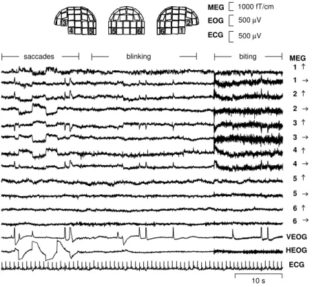
Figure 11 presents a subset of 12 spontaneous MEG signals xi(t) from the frontal, temporal, and occipital
areas (Vigário et al., 1998). The figure also shows the positions of the corresponding sensors on the helmet. Due to the dimension of the data (122 magnetic signals were recorded), it is impractical to plot all the MEG signals
xi(t),i=1, ...,122. Also two electro-oculogram channels and the electrocardiogram are presented, but they were
not used in computing the ICA.
The signal vector x in the ICA model (4) consists now of the amplitudes xi(t)of the 122 signals at a certain
time point, so the dimensionality is n=122. In the theoretical model, x is regarded as a random vector, and the measurements x(t)give a set of realizations of x as time proceeds. Note that in the basic ICA model that we are using, the temporal correlations in the signals are not utilized at all.
The x(t)vectors were whitened using PCA and the dimensionality was decreased at the same time. Then, using the FastICA algorithm, a subset of the rows of the separating matrix W of eq. (6) were computed. Once a vector wihas become available, an ICA signal si(t)can be computed from si(t) =wTix0(t)with x0(t)now denoting the
whitened and lower dimensional signal vector.
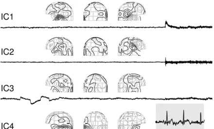
Figure 12 shows sections of 9 independent components (IC’s) si(t),i=1, ...,9 found from the recorded data
together with the corresponding field patterns (Vigário et al., 1998). The first two IC’s are clearly due to the musclular activity originated from the biting. Their separation into two components seems to correspond, on the basis of the field patterns, to two different sets of muscles that were activated during the process. IC3 and IC5 are showing the horizontal eye movements and the eye blinks, respectively. IC4 represents the cardiac artifact that is very clearly extracted.
To find the remaining artifacts, the data were high-pass filtered, with cutoff frequency at 1 Hz. Next, the independent component IC8 was found. It shows clearly the artifact originated at the digital watch, located to the right side of the magnetometer. The last independent component IC9 is related to a sensor presenting higher RMS (root mean squared) noise than the others.
The results of Fig. 12 clearly show that using the ICA technique and the FastICA algorithm, it is possible to isolate both eye movement and eye blinking artifacts, as well as cardiac, myographic, and other artifacts from MEG signals. The FastICA algorithm is an especially suitable tool, because artifact removal is an interactive technique and the investigator may freely choose how many of the IC’s he or she wants.
In addition to reducing artifacts, ICA can be used to decompose evoked fields (Vigário et al., 1998), which en-ables direct access to the underlying brain functioning, which is likely to be of great significance in neuroscientific research.
7.2
Finding Hidden Factors in Financial Data
It is a tempting alternative to try ICA on financial data. There are many situations in that application domain in which parallel time series are available, such as currency exchange rates or daily returns of stocks, that may have some common underlying factors. ICA might reveal some driving mechanisms that otherwise remain hidden. In a recent study of a stock portfolio (Back and Weigend, 1997), it was found that ICA is a complementary tool to PCA, allowing the underlying structure of the data to be more readily observed.
In (Kiviluoto and Oja, 1998), we applied ICA on a different problem: the cashflow of several stores belonging to the same retail chain, trying to find the fundamental factors common to all stores that affect the cashflow data. Thus, the cashflow effect of the factors specific to any particular store, i.e., the effect of the actions taken at the individual stores and in its local environment could be analyzed.
The assumption of having some underlying independent components in this specific application may not be unrealistic. For example, factors like seasonal variations due to holidays and annual variations, and factors having a sudden effect on the purchasing power of the customers like prize changes of various commodities, can be expected to have an effect on all the retail stores, and such factors can be assumed to be roughly independent of each other. Yet, depending on the policy and skills of the individual manager like e.g. advertising efforts, the effect of the factors on the cash flow of specific retail outlets are slightly different. By ICA, it is possible to isolate both the underlying factors and the effect weights, thus also making it possible to group the stores on the basis of their managerial policies using only the cash flow time series data.