Insurance Analytics with Tree-Based Models

(1)

OpenCommons@UConn

Doctoral Dissertations University of Connecticut Graduate School

12-2-2019

Insurance Analytics with Tree-Based Models

Zhiyu Quan

University of Connecticut - Storrs, [email protected]

Follow this and additional works at: https://opencommons.uconn.edu/dissertations

Recommended Citation Recommended Citation

Quan, Zhiyu, "Insurance Analytics with Tree-Based Models" (2019). Doctoral Dissertations. 2374.

(2)

Models

Zhiyu Quan, Ph.D. University of Connecticut, 2019

ABSTRACT

Tree-based models are supervised learning algorithms broadly described by repeated partitioning of the regions of the explanatory variables to form homogeneous groups. The partitioning is based on minimization of a loss function related to the response variable. The results form and create a tree-based structure, which helps make for bet-ter model inbet-terpretation, for predicting the response. Because of the many advantages of tree-based models, their use in disciplines like engineering, biostatistics, and ecology has been a popular alternative predictive tools for building classification and regression models. A single decision tree may not produce accurate predictions, thereby, we also examine the benefits of ensemble methods (e.g., random forests, boosting) for which we produce several trees to improve accuracy. We also describe procedures of tuning model parameters to further improve predictive accuracy. In this thesis, we explore the many potential uses of tree-based models in actuarial science and insurance. First, in valuing large portfolios of variable annuities, we examine the performance of tree-based methods as alternative metamodels for calculating associated guarantees embedded in

(3)

these products. Simulation procedures have been the norm, but tree-based models pro-duce accurate and efficient results that drastically repro-duce the time needed to propro-duce valuation results. Second, for claims predictions in general insurance, we develop the innovative approach of producing hybrid tree-based models, which can be described as a two-step procedure. The first step develops a classification tree-based model for the frequency component, and the subsequent step builds an elastic net regression model for the severity component. This regression is done at each terminal node produced from the classification tree. The resulting hybrid tree structure captures the many benefits of tree-based models and is proposed as an improvement to the existing Tweedie gen-eralized linear model (GLM) widely popular in practice. Finally, we apply multivariate tree models to multi-line insurance claims data with correlated responses. The litera-ture on the theory and relevant uses of building trees with multivariate response is less numerous. However, in building trees as predictive models with multivariate response, we find the potential benefits of better understanding inherent relationships among the several responses and even improvement in marginal predictive accuracy. In the future, to better accommodate the peculiar characteristics of multivariate claim responses, we will further investigate tree-based models using alternative multivariate loss functions.

(4)

Models

Zhiyu Quan

B.S., Xiamen University, China, 2012 M.S., Michigan State University, MI, USA, 2014

A Dissertation

Submitted in Partial Fulfillment of the Requirements for the Degree of

Doctor of Philosophy at the

University of Connecticut 2019

(5)

Copyright by

Zhiyu Quan

(6)

APPROVAL PAGE

Doctor of Philosophy Dissertation

Insurance Analytics with Tree-Based Models

Presented by Zhiyu Quan, B.S., M.S. Major Advisor Emiliano A. Valdez Associate Advisor Guojun Gan Associate Advisor Yuwen Gu University of Connecticut 2019

(7)

Acknowledgements

There are many people without whom this dissertation might not have been accom-plished, and to whom I am much indebted. I would like to express my sincere gratitude to those exceptional individuals who have contributed in many ways and extended un-conditional support during my Ph.D. journey.

Deepest gratitude goes first and foremost to my major advisor Dr. Emiliano A. Valdez for the continuous support of my Ph.D. education, research, and life, and for his understanding, patience, encouragement, enthusiasm, wisdom, and immense knowledge. I would like to acknowledge his efforts to bring me to the University of Connecticut from Michigan State University to continue my Ph.D. program. It was the solid statistic educational support of Michigan State University and the strong actuarial science studies and practices of University of Connecticut that nourished my research perspective. Dr. Valdez encouraged and supported me to seize all the possible opportunities, among which were conferences, seminars, data competitions, and internships, which boosted my research ability and broadened my knowledge. Besides the guidance, Dr. Valdez has been a role model for being a great mentor in life, who had a significant influence on my way of thinking that will benefit me throughout my life. It has been a great honor and privilege of me working with him over the unforgettable five years.

(8)

Dr. Yuwen Gu for the professional guidance and active support to me over the years at the University of Connecticut. Dr. Gan has shown me, by his example, what an excellent researcher and career mentor should be, with timely support and advice. I appreciate Dr. Yuwen Gu for being one of my committee members, for his time, insightful comments, and all the great suggestions that enriched and improved my dissertation.

My sincere thanks also go to all the professors, staffs, and graduate students at Michi-gan State University and the University of Connecticut; thank you for your teaching, enlightening, support, and encouragement. I extend my appreciation to Dr. Lyudmila Sakhanenko, Dr. Albert Cohen, and Sue Watson from Michigan State University, and to Dr. David R. Solomon, Dr. Jeyaraj Vadiveloo, Dr. Fabiana A Cardetti, and Monique Roy from the University of Connecticut for inspiring and simulating discussions.

Furthermore, I am extremely grateful to the funding support from the Society of Actuaries provided in the completion of this research project through our Centers of Actuarial Excellence (CAE) grant on data mining. I would like to thank the feedback from the participants of all of conferences that I have attended. My thanks also go to Gee Lee and Edward W. (Jed) Frees of the University of Wisconsin in Madison who provided the LGPIF data used in this thesis.

Lastly, I wish to thank my loving my family, my parents Hongri Quan, Guiyu Shen, my wife Xianmei Jiang, and my son David Xuanyu Quan, who provide unfailing support and unending inspirations. The time I spent for completing my Ph.D. program could have been time well spent with them; for this reason, I am very grateful.

(9)

List of Tables

1 Validation measures. . . 29

2 Summary statistics of the variables for the training dataset. Dollar amounts are in thousands (’000s). . . 41

3 Grid search results. . . 42

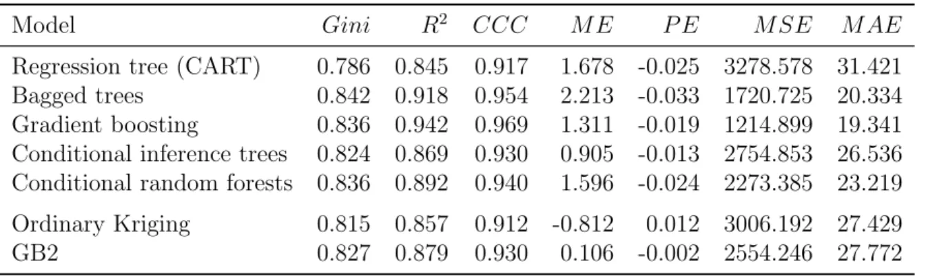
4 Prediction accuracy of different models. . . 48

5 Computational expenses. . . 50

6 Random search and Bayesian optimization. . . 52

7 Prediction accuracy on simulation dataset. . . 78

8 Summary statistics of the variables for the training dataset, 2006-2010. . 80

9 Summary statistics of the variables for the test dataset, 2011. . . 80

10 Regression coefficients at each terminal node. . . 89

11 Description of the six components of the multivariate response variable. . 101

12 Summary statistics of the six components of the multivariate response variable, 2006-2010 (training dataset). . . 103

13 Summary statistics of the explanatory variables, 2006-2010 (training dataset).107 14 Summary statistics of the variables in the 2011 validation dataset. . . 108

15 Comparison of model validation measures. . . 129

(14)

List of Figures

1 Insurance claims: segmentation of explanatory variables. . . 7

2 Insurance claims: segmentation of explanatory variables. . . 7

3 A regression tree. . . 43

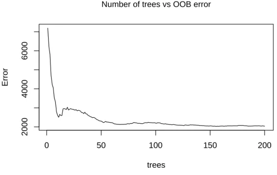
4 Determining the optimal number of trees in bagged trees. . . 44

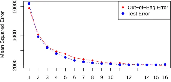
5 Random forests tuning with the number of random subsets (mtry). . . 45

6 A conditional inference trees. . . 47

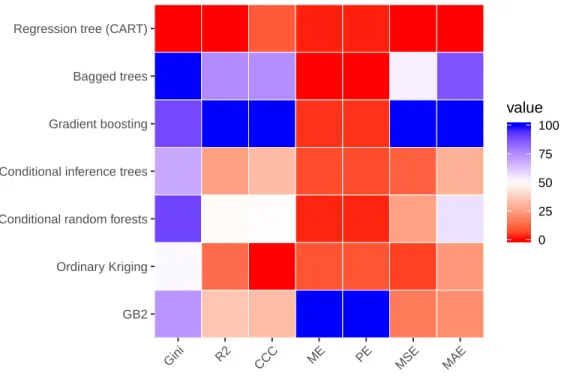
7 A heatmap of model performance according to the various validation mea-sures. . . 49

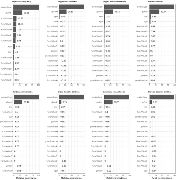
8 Variable importance for tree-based models. . . 53

9 Categorized variable importance for tree-based models. . . 55

10 Lift curve plots. . . 56

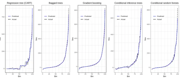
11 Prediction and actual fair market values. . . 58

12 Model performance on training dataset. . . 82

13 Model performance on test dataset. . . 83

14 Classification tree for the frequency. . . 85

15 Tree paths with highlighted nodes. . . 86

16 Classification tree for the frequency. . . 87

(15)

18 Density plots of the logarithm of the positive claim size by type of cover-age, 2006-2010 (training dataset). . . 102 19 Stacked density plots of the logarithm of the claim sizes, including the

zeroes. . . 104 20 Correlations between components of the multivariate response variable. 105 21 Choosing the optimal number of splits. . . 110 22 The optimal univariate regression tree. . . 112 23 Random forests: the number of trees vs the out-of-bag (OOB) error rate. 113 24 Variable importance in random forests regression. . . 114 25 Relative influence of the explanatory variables in gradient boosting. . . 115 26 Choosing the optimal number of splits for the multivariate regression

trees. . . 116 27 The optimal multivariate regression trees. . . 118 28 Multivariate regression tree biplots using PCA to reduce into two

dimen-sions. . . 120 29 Determining the optimal size of the tree for the multivariate tree boosting. 121 30 A heatmap of variable importance using multivariate tree boosting. . . . 122 31 A heatmap of covariance discrepancies for pairs of response variables. . . 123 32 Partial dependence plots of yAvgBC with explanatory variables that are

(16)

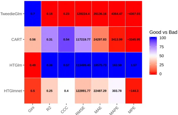
33 Partial dependence plots of yAvgBC with explanatory variables that are not directly associated with the BC coverage. . . 126 34 A heatmap of model performance according to the various validation

(17)

Chapter 1 Introduction

1.1 Objectives

With increasing interest in data science and recent development of state of the art tech-niques in machine learning, insurance companies started to adopt non-traditional models as benchmark models for in house research and development. For example, tree-based models and deep learning models often provide better predictive modeling when com-pared to traditional linear models. Hence, insurance companies compare these machine learning techniques with generalized linear models (GLMs) and other traditional actu-arial techniques. Besides classification and regression framework, insurance companies also use machine learning models for other purposes such as insurance exploratory data analysis and risk factor identification. However, insurance is a highly regulated industry, and the Department of Insurance and state regulators can be hesitant to use machine learning models; they are often considered black-box models and can demonstrate less interpretability compared to traditional approaches. This discrepancy between state reg-ulators and industrial practitioners provides researchers with the opportunity to bridge the gap between industry and state regulation.

(18)

This thesis attempts to bridge this gap between industry and state regulation by exploring the benefits of tree-based models for actuarial and insurance applications. It provides case examples for broadening actuarial toolsets using the tree-based model in order to efficiently evaluate the fair market value for the large portfolio of variable annuity, more accurately price short-term insurance, and model multi-line of businesses claim datasets. Primary efforts and innovations come with tailoring interesting and exciting tree-based models to meet unique characteristics of insurance datasets including right-skewed distributions of claim amount, highly correlated explanatory variables, and many explanatory variables have high missing rate but important to consider in the modeling process, to list a few. The thesis also proposes a new regression framework, termed hybrid tree-based model, as an alternative approach to the traditional two-part regression framework as predictive models for insurance claims.

1.2 Main Contribution

This thesis discusses the advantages of three different applications of tree-based models to the field of insurance. First, we build metamodels to demonstrate the benefits of tree-based models for performing the valuation of guarantees associated with variable annuity (VA) products, especially when used for large portfolios. Results that are based on a synthetic dataset with 190,000 VA contracts indicate that tree-based models are generally efficient in producing accurate predictions and also help to identify important

(19)

risk factors for guarantees embedded in these products. Second, the thesis offers a hybrid tree-based model that improves prediction accuracy compares to conventional methods such as two-part GLM framework or Tweedie GLM. This hybrid structure captures the benefits of tuning hyperparameters at each step of the algorithm, thereby allowing for improved prediction accuracy. Empirical results demonstrate that this hybrid tree-based model produces more accurate predictions without loss of intuitive interpretation and inference. Third, the thesis explores the benefits of multivariate tree-based models when applied to a dataset from the Wisconsin Local Government Property Insurance Fund (LGPIF), which offers multi-line insurance coverage of property, motor vehicles, and contractors’ equipment. These multivariate tree-based models help capture the relationship among the multivariate response variables, and, as results show, improve prediction accuracy in comparison to models based on univariate trees alone.

1.3 Organization of the Thesis

This thesis has been structured as follows. In Chapter 2, we discuss the concept of tree-based models and their historical development. We also examine the actuarial lit-erature that have begun to explore the use of tree-based models for analyzing insurance data. Chapter 3 provides details of parameter tuning, which is an essential process of building tree-based models in order to significantly improve prediction accuracy, espe-cially amongst methods including cross-validation and optimization. In Chapter 4, we

(20)

apply tree-based models as metamodels for the efficient valuation of large variable an-nuity portfolios. Here we also describe another framework of binary splitting generally called unbiased recursive partitioning; conditional inference trees and their extension fall in this category. Furthermore, we compare the performance of various tree-based models, as well as other metamodels, in terms of predictive accuracy and computational efficiency using a synthetic portfolio with large number of VA contracts. Metamodels are considered surrogate models and are used mainly to improve the efficiency of valu-ing embedded guarantees on VA contracts. Chapter 5 introduces the hybrid tree-based model for insurance claims. We use a simulated dataset and a real-life dataset to evalu-ate and compare the model performance between Tweedie GLM and hybrid tree-based models. R implementations for hybrid tree-based models are attached in the appendix. In Chapter 6, we explain the concept of tree-based models when the response variable is multivariate. We describe the multiple lines of business dataset used for our em-pirical investigation and provide some insightful results using multivariate tree-based models. Finally, in Chapter 7, we conclude the findings in this thesis and point out some interesting future research.

(21)

Chapter 2 Traditional Tree-Based Model

Algorithms

2.1 Literature Review

2.1.1 Decision Tree

A decision tree model, with origins that date back to the early 1960s, is a data min-ing algorithm that can broadly be described by repeatedly partitionmin-ing the regions of the explanatory variables and thereby creating a tree-based model for predicting the response. Using survey data, Morgan and Sonquist (1963) developed the very first naive regression tree algorithm and called it the Automatic Interaction Detection (AID).

Since Breiman et al. (1984) introduced the Classification and Regression Tree (CART) algorithm, tree-based models have gained momentum in research and applications in multiple disciplines. The CART algorithm involves separating the explanatory variable space into several mutually exclusive regions that, as a result, it creates a nested hierar-chy of branches resembling a tree structure in which each separation or branch is called

(22)

a node. Each of the bottom nodes of the decision tree, called terminal nodes, have a unique path for data to enter the region. Once the decision tree has been constructed, it is possible to use paths to locate the region or terminal node for which a new set of ex-planatory variables will belong. In accordance with the purpose of predictive modeling, the decision tree algorithm can be divided into the regression tree and the classification tree. According to a survey article by Loh (2014):

“Modern classification trees can partition the data with linear splits on subsets of variables and fit nearest neighbor, kernel density, and other models in the partitions.”

“Regression trees can fit almost every kind of traditional statistical model, including least-squares, quantile, logistic, Poisson, and proportional hazards models, as well as models for longitudinal and multi-response data.”

To illustrate the construction process of a simple regression tree, we use the 64 sets of observed insurance claims data from the R package MASSand took into account three of its potential explanatory variables: Age, District, and Group. In Figure 1, we can see how claims are segmented by Age and District. Note that Group is omitted in this figure because it is not considered as a significant explanatory variable based on the algorithm. Figure 2 shows the final structure of the regression tree generated by the CART algorithm. This tree corresponds to the segmentation of Age and District as demonstrated in Figure 1 where it clearly makes the separation according to shade. This

(23)

0 100 200 300 400 1 Age 0 100 200 300 400 <25 25−29 30−35 >35 0 100 200 300 400 2 District 0 100 200 300 400 1 2 3 4 1 Age: District <25 25−29 30−35 >35 1 2 3 4

Figure 1: Insurance claims: segmentation of explanatory variables.

Insurance claims

Age = <25,25−,30− District = 3,4 11 n=24 35 n=24 129 n=16 yes no

Figure 2: Insurance claims: segmentation of explanatory variables.

illustrates a simple diagram of the separation of nodes within a regression tree model. It can be concluded from these figures that claims are generally significantly larger for age 35 and above than for age under 35, and districts 3 and 4 have slightly lower claims than districts 1 and 2. For similar figures on how decision trees are constructed for classification, see Loh (2014) and Tan et al. (2006).

Hothorn et al. (2006) introduced a conditional inference framework for unbiased re-cursive partitioning which applies stopping criteria based on the statistical permutation

(24)

test (Strasser and Weber, 1999) to address the possible bias in variable selection. This unbiased recursive partitioning framework is applicable to univariate continuous or dis-crete regression, censored regression, classification, ordinal regression, and multivariate regression. The predictive accuracy of this conditional inference trees algorithm has been shown to be comparable to the predictive accuracy of the CART algorithm. For more details about the historical development of decision trees, including alternative algorithms such as GUIDE and C4.5 algorithms, see Loh (2014).

2.1.2 Ensemble Methods of Decision Trees

The early methods of decision trees have potential disadvantage of producing irregu-lar patterns with the result of overfitting. Innovations and extensions to these original methods, such as random forests and gradient boosting, however, improved the capa-bilities of tree-based models to be used as predictive models. Random forests refer to the process of generating ensembles of trees with a set of unpruned fully-grown trees. During this process, these trees are generated based on a bootstrap sampling of the original data and use a subsample of explanatory variables on the each splitting steps. Breiman (2001) showed that the use of random forests led to significant improvements in prediction accuracy.

Boosting algorithms have increased in popularity in machine learning because they can be used to find a good balance between bias and variance through tuning parameters. Boosting algorithms build trees sequentially so that for each new iteration, a tree is grown

(25)

based on residuals from previously grown trees. This procedure combines weak learners to produce strong learners. Early methods of gradient boosting trees, as discussed in Friedman (2002), used optimization based on gradient descent algorithms and this gave rise to the term gradient boosting.

2.1.3 Advantages of Tree-Based Models

Nowadays, the use of tree-based models has become an increasingly popular alternative predictive tool for building classification and regression models. Considered a supervised learning technique, it has many advantages that are especially important for analyzing actuarial and insurance data.

First, tree-based models are considered to be nonparametric and thereby do not require distribution assumptions. In other words, they need not specify the form of explanatory variables to the response variable, unlike classical statistical methods which require the input of certain probability distributions about the response.

Second, tree-based models can be used as a practical algorithm that can handle missing data and categorical variables naturally. This is important because for many real-life datasets, the absence and the unrecording of some information is not uncommon. Furthermore, tree-based models are beneficial because it is otherwise challenging to handle many categorical levels present in traditional statistical modeling.

Third, tree-based models can automatically detect non-linear effects and possible interactions among explanatory variables. Traditional linear models, however, typically

(26)

capture only linear effects, and detection for non-linearity as well as interactions requires further analysis.

Fourth, building tree-based models can produce a variable selection procedure by assessing the relative importance of explanatory variables. Such variable selection is usually vital in actuarial science for purposes of risk classification and collection of risk variables, amongst others.

Finally, decision trees, especially with smaller-sized trees, are straightforward to in-terpret by a visualization of the tree structure in the plot. These advantages are partic-ularly useful for reporting models used in actuarial and insurance data analysis.

Notable, however, is the potentially unsuitable comparison between the predictive accuracy of traditional linear models and decision tree models (and their ensemble meth-ods) because of the differences in their rules and principles. However, in practice, one might make this comparison in order to better evaluate the quality of the models. For example, in the literature which emphasizes applications, there is a direct comparison of prediction accuracy made between traditional statistical models and machine learning algorithms. For example, see Maroco et al. (2011), Mu˜noz and Felic´ısimo (2004), and Thuiller et al. (2003).

(27)

2.1.4 Tree-Based Model Applications in Actuarial Science and

Insurance

We cite some applications of tree-based models in actuarial science and insurance. In-terestingly, for example, Olbricht (2012) provided an alternative look of the life table construction using tree-based models and concluded that tree-based methods have in-herent characteristics to capture intrinsic data structure useful for identifying primary risk factors. Guelman (2012) used the idea of gradient boosting (GB) to predict auto accident loss cost and concluded that this method provided more superior predictive ac-curacy than that of traditional GLM. Guelman et al. (2014) applied conditional inference trees to personalized cross-sell marketing of insurance products, by building personal-ized treatment learning to select profitable policyholders. In particular, the objective of the marketing campaign was to target the optimal group of customers to up-sell the home insurance policies from existing auto insurance policyholders. Deprez et al. (2017) applied the Poisson regression tree and its boosting ensemble to examine the quality of mortality models to understand different causes of death. Lee and Lin (2018) intro-duced Delta Boosting (DB) as an alternative boosting algorithm and showed that this algorithm is optimal under a variety of loss functions. Using claims data on collision coverage for vehicle insurance from a Canadian insurer, the article also demonstrated that the DB algorithm outperforms the GB algorithm. W¨uthrich (2018) illustrated an example of individual claims reserving by using the CART algorithm which is fully

(28)

flexible and considers almost any feature information. In their lecture notes on data an-alytics for non-life insurance pricing, Wuthrich and Buser (2019) used classification trees to determine whether a policy belongs to a male or female driver given specific policy characteristics. Henckaerts et al. (2018) proposed to bin the effects of continuous risk factors with evolutionary trees (Grubinger et al., 2011). Lopez et al. (2019) introduced a new tree-based algorithm to resolve problems in individual claim reserving, especially in the context of long-term risks.

2.2 Traditional Tree-Based Model Algorithms

In this section, we introduce the concept of tree-based models and their extensions under the univariate regression framework. Here we assume the dataset consisting of a vector ofpexplanatory variables, denoted by Xi = (xi1, xi2. . . , xip), which is sampled from the space X = X1 ×. . .× Xp and a response variable, yi, from the sample space as Y, for each ofN observations. This dataset is best represented as (Xi, yi) fori= 1, . . . , N. In the following subsections, we discuss three of the most widely used univariate tree-based models: CART, bagging and random forests, and gradient boosted regression trees.

2.2.1 Classification and Regression Trees (CART)

The CART algorithm (Breiman et al., 1984) uses a greedy search called recursive binary partition to create a tree structure. In conventional terms, the trees obtained by the

(29)

algorithm are called classification trees when the response variable is categorical and they are called regression trees when the response variable is continuous.

We adopt notation from Hastie et al. (2009). In the CART algorithm, a regression tree, denoted byT(X; Θ), is produced by partitioning the space of explanatory variables,

X, into M disjoint regions R1, R2, . . . , RM and then assigning a constant cm as the predicted value for each region Rm, for m = 1,2, . . . , M. Given a regression tree, each observation can then be modeled based on the expression

f(X|Θ) =T(X; Θ) = M

X

m=1

cm1Rm(X), (2.1)

where Θ = {Rm, cm}Mm=1 denotes the partition with the assigned constants. Under the

CART algorithm, constantscm are determined by minimizing the sum of squared errors (SSE) loss function:

L(yi,byi) = N X i=1 (yi−byi) 2_, _(2.2) where _byi =fb(X_i|Θ) = PM

m=1bcm1Rm(Xi) is the predicted value of the response variable.

It can be shown that the optimal value, _bcm, is the average ofyi in the regionRm:

bcm = average(yi|Xi ∈Rm) = 1 Nm X Xi∈Rm yi, (2.3)

(30)

The regions in the regression tree are determined according to recursive binary split-ting. The initial step in this algorithm is to find one explanatory variable x·j which best divides the data into two subregions. For example, RL(j, s) = {Xi|x·j < s} and RR(j, s) ={Xi|x·j ≥s} in the case of a continuous explanatory variable. This division is determined as the solution to

argmin j,s X i:Xi∈RL(j,s) (yi−bcRL(j,s)) 2₊ X i:Xi∈RR(j,s) (yi−bcRR(j,s))

2_, _{for any} _j _and _s.

Subsequently, the algorithm looks for the next explanatory variable with the best division of two subregions and this process is applied recursively until reaching a minimum size of observations in the terminal region or some other predefined threshold. The algorithm can handle other types of numerical explanatory variables, such as those with rank order, as well as categorical variables. Furthermore, regression trees can deal with missing values in explanatory variables using surrogate splitting which involves finding a surrogate variable that best approximates the original split. In other words,surrogate

splitting finds an alternative explanatory variable to mimic the explanatory variable that

contains missing values. Hence, observations with missing values are assigned according to the split on the surrogate variable rather than on the original splitting variable. The

surrogate splitting process also provides variable importance at each node by measuring

the decrease of the error function.

(31)

that may lead to overfitting and unnecessary model complexity. This complexity can be controlled by using cost-complexity pruning to trim the fully grown tree T0. From

equations (2.2) and (2.3), we can define the loss in the region Rm by

Lm(T) = 1 Nm X Xi∈Rm (yi−bcm) 2_.

For any subtreeT ⊂T0, we denote the number of terminal regions in this subtree by|T|.

To control the number of terminal regions, we introduce the tuning parameterα ≥0 to the loss function by defining the new cost function as

Cα(T) =

|T|

X

m=1

NmLm(T) +α|T|.

Clearly according to this cost function, the tuning parameter penalizes a large number of regions. The idea then is to find the subtrees Tα ⊂ T0 for each α, and choose

the subtree that minimizes Cα(T). Furthermore, the tuning parameter α governs the tradeoff between the size of the tree and its goodness of fit to the data similar to the regularization parameter in a penalized regression. Large values of α result in smaller

trees and as the notation suggests,α= 0 leads to the fully grown treeT0. The estimation

of this tuning parameter α is done usingk-fold cross-validation.

Algorithm 1 summarizes the details of implementing the CART algorithm procedure using the R-package rpart. See James et al. (2013a), and Therneau et al. (2015).

(32)

Algorithm 1: CART R-package: rpart

Input: Training dataset X,y, K

Output: Best subtree Tα

1 Grow a full tree T₀ on a training dataset using recursive binary splitting. Use the

stopping criterion minsplit which is the minimum number of observations in a region for a split to be attempted;

2 Prune the full tree T₀ to subtrees T_α using cost-complexity pruning; 3 Divide the training dataset into K folds to determine the optimal tuning

parameter α;

4 for k= 1, . . . , K do

5 Repeat steps 1 and 2 on all except for the k-th fold;

6 Compute the mean squared prediction error on the hold outk-th fold usingT_α; 7 end

8 Average the results for each value of α and pick α that minimizes the average

prediction error;

9 Return the best subtree T_α;

2.2.2 Bagging and Random Forests

Bagging (Breiman, 1996) uses an ensemble of sufficiently deep, unpruned CART trees,

{T(X; Θb), b = 1,2, ..., B} which are generated based on a bootstrap sampling from the original training dataset. As a result, we can think of{Θb}as independent and identically distributed random vectors. WithB as the total number of bootstrap samples, we define

the model for the response variable as the average of all of the regression trees in bagging:

fB(X|Θ) = 1 B B X b=1 T(X; Θb).

Random forests first developed by Breiman (2001) further reduce the correlation between CART trees by selecting the best split from a random subset of explanatory variables at each node of a tree. The size of the random subset of explanatory variables

(33)

Algorithm 2: R-package: randomForest

Input: Training dataset X,y, B

Output: {T(X; Θb), b= 1,2, ..., B}

1 for b= 1, . . . , B (ntree) do

2 Draw a bootstrap sample of size sampsize from the training data;

3 Grow a full tree T(X; Θb) on the bootstrap sample using recursive binary splitting and selecting mtry variables at random from the pexplanatory variables with stopping criterion nodesize;

4 end

5 Return the ensemble of trees {T(X; Θ_b), b = 1,2, ..., B}; 6 Average fB(X|Θ) =

1 B

PB

b=1T(X; Θb);

can be optimally chosen through cross-validation; some use the rule of thumb such as the square root of the total number of explanatory variables, √p, in the training dataset. In effect, the average prediction of multiple CART trees is expected to have a lower variance than a single individual CART tree. Larger random sets of explanatory variables can improve the predictive capability of individual trees, but they can also increase the correlation between trees and void any gains from averaging multiple predictions. The bootstrap resampling of the data for training each tree also increases the variation between the trees. The accuracy of random forests depends on the strength of each individual tree and the measure of the dependence between them. By the Strong Law of Large Numbers, as B → ∞, we have

EX,y(y−fB(X|Θ))2 →EX,y(y−Eθf(X|Θ))2 a.s.

(34)

why they do not overfit as the increase of the trees.

For implementing random forests in R, see Liaw and Wiener (2002). The procedure to produce random forests is summarized in Algorithm 2.

2.2.3 Gradient Boosted Regression Trees

Developed by Friedman (2001), the gradient boosting algorithm grows trees by sequen-tially putting more weights on the residuals from previous trees. For each new iteration in the sequential process, a regression tree is grown using information from previously grown regression trees. In other words, each subsequent regression tree focuses on learn-ing from the residuals obtained from previous trees. The result is a set of S regression

treesT(X; Θs), fors= 1, . . . , S. The gradient boosted regression tree model is expressed as the sum of these trees:

FS(X|Θ) = S

X

s=1

T(X; Θs),

Here, S is also referred to as the number of iterations in the process. For each step s,

we find the optimal Θs by solving the problem:

b Θs = arg min Θs N X i=1 L(yi, Fs−1(Xi|Θ) +T(Xi; Θs)). (2.4) We note that Fs(Xi|Θ) =b F_s−1(Xi|Θ) +b Ms X m=1 b cms1Rms(Xi),

(35)

where_bcms = arg min c

P

Xi∈RmsL(yi, Fs−1(Xi|Θ) +c).

Under SSE loss function, it simplifies to the regression tree so that best predicts the current residuals yi −Fs−1(Xi|Θ), andb

b

cms is the mean of these residuals in each corresponding region.

For other differentiable loss functions, the solution to equation (2.4) can be obtained by numerical optimization via gradient boosting as described in Friedman (2001). The regression treesTs(X; Θs) produced at each step are analogous to the components of the negative gradient: gis =−∇fs−1L(yi, Fs−1(Xi|Θ)) =− ∂L(yi, F(Xi|Θ)) ∂F(Xi|Θ) F(Xi|Θ)=Fs−1(Xi|Θ) for i= 1, . . . , N.

Therefore, solving equation (2.4) is equivalent to solving the following:

Fs(Xi|Θ) =Fs−1(Xi|Θ) +γs N X i=1 gis where γs= arg min γ N X i=1 L(yi, Fs−1(Xi|Θ) +γgis)

Gradient boosted regression trees can be implemented using the R package gbm. See Ridgeway (2007a), and Ridgeway (2007b). The process is summarized in Algorithm 3.

(36)

Algorithm 3: R-package: gbm

Input: Training dataset X,y, B

Output: FS(X|Θ) =

PS

s=1λfs(X|Θs)

1 for s= 1, . . . , S (ntree) do

2 for i= 1, . . . , N ∗p (p isbag.f raction) do 3 Compute g_is =−∇_F_s₋₁L(y_i, F_s−1(Xi|Θ));

4 Fit a regression tree Ts(X; Θs) to the targets gis giving terminal regions R1, R2. . . , RMs: interaction.depth=Ms and stopping criteria is

n.minobsinnode; 5 for m= 1, . . . , Ms do 6 compute b cms = arg min c P Xi∈RmsL(yi, Fs−1(Xi|Θ) +c); 7 end 8 end 9 Update F_s(X_i|Θ) =F_s−1(Xi|Θ) +λ PMs m=1cms1Rms(Xi) where shrinkage λ is

used to reduce the impact of each additional fitted base-learner, regression tree, Ts(X; Θs).

10 end

(37)

Chapter 3 Hyperparameter Optimization of

Tree-Based Models

3.1 Tree-Based Model Hyperparameters

We include hyperparameters optimization as a stand-alone chapter for the purpose of a self-contained thesis. It is also beneficial for providing all the essential techniques in-volved in tuning machine learning models. Table 16, in the appendix, lists some common tuning hyperparameters for tree-based models mentioned in this thesis. Hyperparameter optimization is the process of building flexible tree-based models that fit the underlying dataset. Without a proper fine-tuning process, the prediction accuracy of tree-based models may not outperform other traditional predictive models.

3.2 Cross-Validation

Hyperparameter tuning (optimization) of tree-based models usually involves cross-validation to perform model selection. Cross-validation was introduced to fix the overoptimistic

(38)

prediction accuracy on the same dataset trained by the model. In other words, it is an attempt to avoid overfitting. See Mosteller and Tukey (1968), Stone (1974), and Geisser (1975).

Cross-validation is a way to examine tree-based model performance on hypothetical validation dataset when an exact validation set is not available. In detail, the dataset is separated into two disjoint parts: training dataset and validation dataset. The model is built on the training dataset and the prediction performance is examined on the validation dataset.

Various splitting strategies lead to different cross-validation techniques. Data split-ting requires certain assumptions. For example, data are identically distributed and there must be independence between training dataset and validation dataset. If these as-sumptions are not satisfied, then some modifications are needed for the cross-validation. See Opsomer et al. (2001), and Leung et al. (2005). Usually for insurance datasets, time dependency and outliers are present. It requires extra attention when we apply general cross-validation to perform model selection.

In the holdout method (Devroye and Wagner, 1979), the dataset is separated only once, and typically the validation dataset is smaller than the training dataset. The holdout method can be considered as the simplest cross-validation. While the holdout method suffers from a drawback that the results highly depend on data split, it is because the data in the validation dataset may have important information and this information is left out when we train model. In other words, the data segment easily leads to bias

(39)

in the result. To deal with this issue, other cross-validation is discussed later.

Unlike the holdout method, other cross-validation generally splits dataset several times and averages prediction accuracy on validation dataset. The question arises on how to split the dataset. There are two types of splitting: exhaustive data splitting and partial data splitting.

3.2.1 Exhaustive Cross-Validation

Exhaustive cross-validation methods contain training and testing on all possible ways to divide the original dataset into a training dataset and a validation dataset. See Stone (1974), Allen (1974), Geisser (1974), and Shao (1993). There are two popular exhaustive cross-validation:

• Leave-one-out. Each data point is withdrawn from the original dataset and used as validation data. Obviously, it needs n runs. Leave-one-out cross-validation

provides nearly unbiased estimation while it suffers from high variance.

• Leave-p-out. Here p data points are withdrawn from the original dataset and it takes N_p

runs. In practice, for large dataset, exhaustive cross-validation is computationally intensive.

(40)

3.2.2 Non-Exhaustive Cross-Validation

Non-exhaustive cross-validation apply partial data splitting. One well-known non-exhaustive cross-validation is k-fold cross-validation, see Geisser (1975). In k-fold cross-validation,

the original dataset is segmented into k equal sized subsamples. In each run, one of

the k subsamples is held out as validation dataset and model is built on the remaining

k−1 subsamples. In total, there arek runs with each subsample selected only once as validation dataset. This process assures all the data points have a chance to belong in the training dataset and the validation dataset. This method takes the average of the prediction results from thek validation datasets.

When k is equal to the number of the dataset, the k-fold cross-validation becomes

the leave-one-out cross-validation. It is an open question to choose the best k for the

k-fold cross-validation. If the number k is selected, then the size of the training set is

fixed as well as the number of splits. The bias of the k-fold cross-validation decreases

with k since larger k leads to a larger training set. On the other hand, the variance

of the k-fold cross-validation increases withk since a larger k leads to a larger number

of validation procedure (i.e., more runs). Practically, the number k is often chosen to

be between 5 and 10. 10-fold cross-validation has been shown to provide good model selection and point estimation. See Kohavi et al. (1995).

Additional cross-validation techniques and statistical properties of cross-validation are discussed in Arlot and Celisse (2010) and Leung et al. (2005).

(41)

3.3 Hyperparameter Optimization

3.3.1 Grid Search

Grid search is the most traditional way to optimize hyperparameters. It is an exhaustive searching process on the manually specified subset of hyperparameter space. The selec-tion of the best combinaselec-tion of hyperparameters is usually based on the cross-validaselec-tion. Determining the subset involves setting bounds and discretization that requires exper-tise on the model. Grid search is computationally intensive due to the explosive number of combinations of hyperparameters. For example, if one model has p parameters and

each parameter hascchoices, then the subset containscp_{combinations. Fortunately, grid} search is essentially parallel since evaluating each combination of the hyperparameters is independent of each other. This makes grid search feasible given enough computational power.

3.3.2 Random Search

Random search is to randomly search the grid of hyperparameters that is manually specified and it has similar performance compared to the grid search. It can outperform the grid search given the same computation constraint and time, especially when only a small number of hyperparameters affects the final performance of the model, see Bergstra and Bengio (2012). In other words, if the close-to-optimal region of hyperparameters occupies at least 5% of the search space, then a random search with a certain number

(42)

of trials (typically 40-60 trials) will be able to find that region with high probability. Like grid search, it can be made parallel. When compared to grid search, random search requires less number of trials and allows including prior knowledge of how to sample.

3.3.3 Automatic Hyperparameter Optimization

Automatic hyperparameter tuning establishes knowledge about the association between the hyperparameter settings and model performance to improve selection for the next hyperparameter settings. Unlike previously discussed tuning methods, the selection of the following hyperparameter settings is no longer independent of the prior selection. In other words, it is sequential. Hence it cannot be easily made parallel. The hy-perparameter tuning becomes an optimization problem. There are several sequential global optimization methods for finding the hyperparameter setting that maximize the model generalization performance. One of the most popular techniques is Bayesian opti-mization. Bayesian optimization models generalization performance as a sample from a Gaussian Process (GP) (Snoek et al., 2012), and creates a regression model to formalize the relationship between the model performance and the model hyperparameters.

Specifically, let function f : H → _R model hyperparameter setting h ∈ H to a prediction accuracy of

hoptimal = arg max h∈H

(43)

within a domain h ∈ _Rd _{which is a bounding box.} _d _{is the number of tuning} hyperpa-rameters. The functionf is a realization of a GP with meanµand covariance kernelK,

i.e., f ∼ GP(µ, K). The Bayesian optimization assumes that the prediction follows the normal distribution. After choosing the kernel function K, we can compute the mean

and variance for this normal distribution. For further details, see Snoek et al. (2012), and Martinez-Cantin (2014).

There are also a few other automatic hyperparameter optimization techniques: gradient-based, evolutionary and those based on tree-structured Parzen estimator. Gradient-based optimization computes the gradient with respect to hyperparameters and then optimizes the hyperparameters using gradient descent. See Bergstra et al. (2011), and Larsen et al. (1996).

3.4 Validation Measures

There are several prediction accuracy measures but there is no unique perfect measure that can be used to judge prediction accuracy under all circumstances. Each measure has its own focus, which also leads to its shortcomings. For example, the mean squared error has the disadvantage of the heavy focus on outliers since it is a result of the squaring of each term. This shortcoming is undesirable in many applications, especially in general insurance with large claims. It has led us to use alternatives such as the mean absolute error, or those based on the median. The concordance correlation coefficient measures

(44)

the correlation between two variables without directly comparing the magnitude of actual values. Frees et al. (2011) and Frees et al. (2014b) applied the Gini index as a validation measure in the insurance context. In insurance datasets, it is common to observe a mixture of zeros corresponding to no claims and a right-skewed distribution with thick tails due to the massive claims. Gini index extends the classical Lorenz curve, defined as twice the area between the curve and the 45-degree line. For a given ordering, a large Gini index signals a significant difference between two distributions. For further discussion, see Denuit et al. (2019).

To make a fair comparison between different models, we utilize a few popular mea-sures in this thesis. These meamea-sures are: Gini index, coefficient of determination R2,

concordance correlation coefficient (CCC), mean error (ME), mean percentage error (MPE), percentage error (PE), mean squared error (MSE), root mean squared error (RMSE), mean absolute error (MAE), and mean absolute percentage error (MAPE). These validation measures are each defined in Table 1 with its interpretation.

(45)

Table 1: Validation measures.

Validation measure Description Interpretation

Gini Index Gini= 1− 2

N−1 N− PN i=1 i˜yi PN i=1y˜i !

Higher Gini is better. where ˜yis the corresponding toyafter

ranking the corresponding predicted valuesy_b. Coefficient of Determination R2_{= 1}₋ PN i=1(ybi−yi) 2 PN i=1 yi− 1 n Pn i=1yi 2 HigherR 2_{is better.}

where_byis predicted values. Concordance Correlation CCC= 2ρσyibσyi σ2 b yi+σ 2 yi+(µyib− µ_yi)2 Higher CCC is better. Coefficient whereµybi andµyi are the means

σ2

b

yi andσ

2

yi are the variances

ρis the correlation coefficient

Mean Error M E= 1

N

PN

i=1(ybi−yi) Lower|M E|is better. Mean Percentage Error M P E= 1

N PN i=1 b yi−yi yi Lower|M P E|is better. Percentage Error P E= PN i=1byi− PN i=1yi PN i=1yi Lower|P E|is better. Mean Squared Error M SE= 1

N

PN

i=1(byi−yi)

2 _Lower_{M SE} _{is better} Root Mean Squared Error RM SE=

r 1 N PN i=1(ybi−yi) 2 _Lower_{RM SE} _{is better} Mean Absolute Error M AE= 1

N

PN

i=1|byi−yi| LowerM AEis better. Mean Absolute Percentage Error M AP E= 1

N PN i=1 b yi−yi yi LowerM AP E is better.

(46)

Chapter 4 Efficient Valuation of Large Variable

Annuity Portfolios

4.1 Introduction

A variable annuity (VA) is a tax-deferred retirement vehicle that is created by insur-ance companies to address concerns many people have about outliving their assets. VA policies typically contain guarantees, which include guaranteed minimum death benefit (GMDB), guaranteed minimum accumulation benefit (GMAB), guaranteed minimum income benefit (GMIB), and guaranteed minimum withdrawal benefit (GMWB), see Hardy (2003). These guarantees provide policyholders downside protection during sig-nificant declines in the financial market. As a result, these are financial guarantees that cannot be adequately addressed by traditional actuarial approaches. For example, dur-ing a bear market when stock prices are falldur-ing, insurance companies can expect to lose large sums of money on their portfolios of VA policies.

(47)

risks associated with VA guarantees. An important step of dynamic hedging is to quan-tify the risks, which involves calculating the fair market values of the guarantees. Since the guarantees are complex, their fair market values cannot be determined explicitly or in closed form. In practice, insurance companies resort to Monte Carlo simulation to calculate the fair market values of guarantees. Monte Carlo simulation is flexible and can handle any types of guarantees, but it is computationally intensive. Hence, using Monte Carlo simulation to calculate the fair market values of a large portfolio of VAs can take days or weeks.

To speed up the valuation of VA portfolios based on Monte Carlo simulation, meta-modeling techniques have been proposed in the past few years. See Gan and Lin (2015), Gan and Valdez (2017a), Hejazi et al. (2017), Gan and Huang (2017), Gan (2018), and Xu et al. (2018). Metamodeling techniques involve building a predictive model based on a small number of representative VA policies in order to reduce the number of poli-cies that are valued by Monte Carlo simulation. Specifically, a metamodeling technique consists of the following four components:

1. Select a small number of representative VA policies;

2. Use Monte Carlo simulation to calculate the fair market values of the representative policies;

3. Build a predictive model, called a metamodel, based on the representative policies and their fair market values; and

(48)

4. Use the predictive model to estimate the fair market value for every VA policy in the portfolio.

Since only a small number of VA policies are valued by Monte Carlo simulation and the predictive model is much faster than Monte Carlo simulation, metamodeling techniques have the potential to reduce the valuation time significantly.

In the past, ordinary kriging (Gan, 2013), universal kriging (Gan and Lin, 2017), GB2 (Generalized beta of the second kind) regression model (Gan and Valdez, 2018), and neural networks (Hejazi and Jackson, 2016; Xu et al., 2018) have been used to build various types of metamodels. Kriging is a family of estimators used to interpolate spatial data. Advantages of kriging methods include producing accurate aggregate results at the portfolio level and requiring only a few parameters to estimate. However, kriging methods have disadvantages that they require a large number of distance calculations and assume normal distribution of the response variable. The GB2 regression model has the advantage that it can handle highly skewed data, but estimating parameters poses quite a challenge. Neural networks have several advantages: they can approximate any compactly supported continuous function arbitrarily well; they can model data that has nonlinear relationships between variables; and they can handle interactions between variables. However, handling categorical variables (especially categorical variables with multiple categories) in neural networks is not as straightforward as that in tree-based models.

(49)

4.2 Unbiased Recursive Partitioning

The CART algorithm described in Section 2.2.1 employs the recursive binary partition. This greedy search causes some drawbacks. One drawback is overfitting, which can be resolved using a pruning process by applying cross-validation. Another drawback is the resulting bias in variable selection, especially when the explanatory variables present many possible splits or missing values. This latter drawback is harder to remedy. Our variable annuity dataset presents many types of embedded guarantees. If we use the CART algorithm directly may cause bias in variable selection. Hence, we are introducing the unbiased recursive binary partition in the following subsections.

4.2.1 Conditional Inference Trees

The main difference between the CART algorithm and conditional inference trees al-gorithm is the variable selection at each split and the stopping criterion. To explain the details, we need to define a few terms. The conditional distribution of a statistic, F(Y|X), measures the association between the response variable and the explanatory variables. Each observation in the dataset can form a learning sample denoted by Ln:

Ln={Yi, xi1, xi2. . . , xip}ni=1

It is possible that some explanatory variables xij are missing in real-life data. The tree-based model ultimately finds membership for observations and assigns them to the

(50)

terminal node, Rm. To define this membership for each observation, we introduce the vector of case weights denoted byw= (w1, . . . , wn). Hence, for each terminal node,Rm, we have a vector of case weightsw= (w1, . . . , wn). The weight,wi, can be any positive value if it is an observation in the specific terminal node. Without loss of generality, we can restrict the weight value to either one or zero. Define symmetric group, S(Ln,w), as all possible permutations of observations with weight one. For example, if w1 =

1, w2 = 0, w3 = 1, w4 = w5 = . . . = wn = 0, then S(Ln,w) = {(Y1, x11, x12, . . . , x1p), (Y3, x31, x32, . . . , x3p), (Y3, x11, x12, . . . , x1p), (Y1, x31, x32, . . . , x3p)}.

We now briefly describe unbiased recursive binary splitting. First, under a specific vector of case weights, apply statistical hypothesis test to determine if there is any dependency between the response variable and the explanatory variables. If there is a dependency, then find the most significant (strongest association) explanatory variable to perform the split and update the case weights. If there is no dependency, then stop the process.

In formulating the process, the null hypothesis is that all the explanatory variables are independent of the response variable

H0 =∩

p j=1H

j

0,

where H₀j :F(Y|X·j) = F(Y). Then use the conditional distribution of linear statistics in the permutation test, see Strasser and Weber (1999). The linear statistic,TXj(Ln,w)

(51)

measures the association between the response variable and the j-th explanatory vari-able: TX·j(Ln,w) =vec n X i=1 wigj(xij)h(Yi,(Y1, Y2, . . . Yn))T ! ∈_Rpjq

where gj : X·j → Rpj is a nonrandom transformation of the explanatory variable X·j. Under univariate continuous regression framework, this transformation function can be the identity function, the rank function, or the nonlinear function for numeric explana-tory variables. For a categorical explanaexplana-tory variable, the transformation function can be based on a “dummy coding”. Theinfluence function is defined ash:Y × Yn_→

Rq.

The most common influence function is the identity functionh(Yi,(Y1, Y2, . . . Yn) =Yi. If there are extreme values in the response variable, the influence function can be the rank function h(Yi,(Y1, Y2, . . . Yn) =Pn_s₌₁wsI(Ys≤Yi). The vecfunction converts matrix to vector.

Under H0 and given all permutations of the response variable, the conditional

ex-pectation µj ∈Rpjq can be derived as follows:

µj =E(TX·j(Ln,w)|S(Ln,w)) =vec(( n X i=1 wigj(xij))E(h|S(Ln,w))T) (4.1) where E(h|S(Ln,w)) = 1 Pn i=1wi n X i=1 wih(Yi,(Y1, Y2, . . . Yn))

(52)

and the covariance Σj ∈Rpjq×pjq can be derived as Σj =V(TX·j(Ln,w)|S(Ln,w)) = Pn i=1wi Pn i=1wi−1 V(h|S(Ln,w))⊗( n X i=1 wigj(xij)⊗wigj(xij)T) −_P_n 1 i=1wi−1 V(h|S(Ln,w))⊗( n X i=1 wigj(xij))⊗( n X i=1 wigj(xij))T (4.2) where V(h|S(Ln,w)) = 1 Pn i=1wi n X i=1 wi(h(Yi,(Y1, Y2, . . . Yn))−E(h|S(Ln,w))) ·(h(Yi,(Y1, Y2, . . . Yn))−E(h|S(Ln,w)))T

where ⊗ is the Kronecker product.

The linear statistic, TX.(Ln,w), can be standardized since TX.(Ln,w)−µ.is

asymp-totically normal under H0 and conditioned on the symmetric σ-fields S(Ln,w). See Strasser and Weber (1999). There are a few ways of standardization mentioned in Hothorn et al. (2006). One way is based on the maximum of the absolute values of the standardized linear statistics defined by

zmax(TX., µ.,Σ.) = max k=1,2,...,pq (TX. −µ.)k diag(Σ.)1/2 .

(53)

Another way is based on the quadratic form defined by zquad(TX., µ.,Σ.) = (TX. −µ.)Σ + . (TX. −µ.) T_, where Σ+

. is the Moore-Penrose inverse of Σ. which may be computationally intensive. The Moore-Penrose inverse is the most common type of pseudo-inverse. See Moors (1920), and Penrose (1955). For the case of the quadratic form, the test statistic asymp-totically follows a chi-squared distribution with rank(Σ.) degrees of freedom.

Since the test statistic z(TX., µ.,Σ.) cannot be compared directly due to possibly

difference of scale in the explanatory variables, we use the p-value to choose the most

significant explanatory variable. We select explanatory variable,Xj∗, that has the

small-estp-value, Pj∗ = arg min

j=1,...,p

Pj, where

Pj =PH₀j(z(TXj, µj,Σj)≥z(tXj, µj,Σj)|S(Ln,w))

and tXj ∈R

pjq _{is the observed test statistic from the dataset.}

After picking the best explanatory variableXj∗, we then find the best splitting point

according to the splitting criterion. This criterion can be a simple binary split like the CART algorithm, or a multiway split as in O’Brien (2004). We can also utilize the permutation test framework to find the best split point. For all possible split of the space Xj∗, denote this as A and Ac. For a given subset A, the linear statistic can be

(54)

written as T_XA ·j∗(Ln,w) = vec n X i=1 wiI(xij∗ ∈A)h(Y_i,(Y₁, Y₂, . . . Y_n))T ! ∈_Rq

According to Equations 4.1 and 4.2, µA

j∗ and ΣA_j∗ can be calculated. Then the best

split,A∗, that maximizes the test statistic over all possible splits can be found as follows:

A∗ = arg max A z(T_XA j∗, µ A j∗,ΣA_j∗)

Given a predefined significance level,α, if the null hypothesis,H0, cannot be rejected,

then stop the binary splitting process. Here, the p-value for the null hypothesis can be

calculated using the Bonferroni-ajustedp-value(1−(1−Pj)p) or min-p-value resampling. For more advanced multiple testing, we refer the reader to Westfall and Young (1993).

The level of significance, α, controls the tree size. It can be tuned using

cross-validation and this process can be similar to tree pruning in the CART algorithm. In detail, one would initially set higher significance level, α, which leads to a larger tree,

and then prune the terminal node by setting a lower significance level, α∗ ≤ α. The significance level can be predetermined according to a tolerance based on some actuarial expertise. Moreover, the significance level can be interpreted in the traditional statistical sense of balancing the Type I and Type II errors.

(55)

4.2.2 Bagging and Random Forests Using Conditional

Infer-ence Trees as Base Learner

Random forests, especially ensemble on CART trees, variable importance provides es-sential interpretation for the ensemble tree-based models although it is not reliable to perform variable selection according to variable importance scores. This is especially true for cases where the explanatory variables vary in the scale of measurement or number of categories. See Strobl et al. (2007). On the other hand, conditional random forests are created based on conditional inference trees that can provide unbiased variable selection. The framework of conditional random forests is very similar to that of random forests. The conditional inference trees are built on the bootstrap sample or subsample of the original dataset. The random subset of the explanatory variables is considered at each split. However, there are few differences between conditional random forests and random forests. First, after building all the conditional inference trees, the final ensemble model averages the observation weights extracted from each tree. It is a different aggregation scheme from the random forests which simply averages the prediction. Second, condi-tional random forests can extensively model censored, multivariate, as well as ordered response variable. Third and finally, when explanatory variables vary in their scale of measurement and the number of categories, which is very typical of a dataset, the con-ditional random forests can provide unbiased variable selection and variable importance based on conditional inference trees that use subsamples without replacement.

(56)

4.3 Variable Annuity Valuation

4.3.1 Data Description

We use the hierarchicalk-means algorithm mentioned in Nister and Stewenius (2006) to

select the representative VA policies. The dataset is a synthetic dataset that contains 190,000 VA policies. For details, see Gan and Valdez (2017b). We select 680 VA contracts from the dataset as training dataset, select 340 VA contracts as validation dataset and perform prediction on the 190,000 VA contracts. We select validation dataset to speed up the hyperparameter tuning process and model selection. Some summary statistics of the training dataset are provided in Table 2.

4.3.2 Grid Search Results

For all the model calibration, we train the model on the training dataset (680 VA contracts). Since the dataset is scalable, it allows us to perform grid search and 10-fold cross-validation. All the hyperparameters mentioned below are the grid search results.

For the regression tree, we grow a full tree using recursive binary splitting with a minimum number of five observations in a region for a split to be attempted. Then we prune this fully grown tree using cost-complexity pruning with “one standard deviation rule” regularization parameter of 1.084e-02.

In detail, as mentioned in Table 16, we tune two common tuning hyperparameters “cp” and “minsplit” for the regression tree base on the training dataset using 10-fold

(57)

Table 2: Summary statistics of the variables for the training dataset. Dollar amounts are in thousands (’000s).

Response

variables Description Min. 1st Q Mean Median 3rd Q Max. fmv Fair market value -68.37 -5.55 64.63 11.7 64.84 1210.32 Continuous

variables

gmwbBalance GMWB balance 0 0 27.8 0 0 422.26 gbAmt Guaranteed benefit amount 51.88 183.98 323.29 306.89 437.36 920.62 FundValue1 Account value of the 1st fund 0 0 32.02 12.62 46.76 629.89 FundValue2 Account value of the 2nd fund 0 0 36.54 16.08 56.31 571.59 FundValue3 Account value of the 3rd fund 0 0 26.78 11.81 36.64 458.78 FundValue4 Account value of the 4th fund 0 0 25.8 10.48 38.29 539.36 FundValue5 Account value of the 5th fund 0 0 22.29 10.54 34.71 425.92 FundValue6 Account value of the 6th fund 0 0 37.15 19.64 53.96 654.64 FundValue7 Account value of the 7th fund 0 0 28.78 12.88 42.56 546.89 FundValue8 Account value of the 8th fund 0 0 31.27 15.59 46.24 529.57 FundValue9 Account value of the 9th fund 0 0 31.93 13.9 45.17 599.44 FundValue10 Account value of the 10th fund 0 0 32.6 13.86 45.09 510.43 age Age of the policyholder 34.52 42.86 50.29 51.36 57.21 64.46 ttm Time to maturity in years 0.75 10.09 14.61 14.6 19.12 27.52 Categorical

variables Description Proportions

gender.M Male policy holder 64.71 %

gender.F Female policy holder 35.29 %

productType.ABRP Indicate type GMAB with return of premium 8.82 % productType.ABRU Indicate type GMAB with annual roll-up 4.26 % productType.ABSU Indicate type GMAB with annual ratchet 6.03 % productType.DBAB Indicate type GMDB + GMAB with annual ratchet 5.00 % productType.DBIB Indicate type GMDB + GMIB with annual ratchet 5.88 % productType.DBMB Indicate type GMDB + GMMB with annual ratchet 5.74 % productType.DBRP Indicate type GMDB with return of premium 4.85 % productType.DBRU Indicate type GMDB with annual roll-up 6.62 % productType.DBSU Indicate type GMDB with annual ratchet 4.41 % productType.DBWB Indicate type GMDB + GMWB with annual ratchet 4.41 % productType.IBRP Indicate type GMIB with return of premium 5.74 % productType.IBRU Indicate type GMIB with annual roll-up 4.71 % productType.IBSU Indicate type GMIB with annual ratchet 4.85 % productType.MBRP Indicate type GMMB with return of premium 4.56 % productType.MBRU Indicate type GMMB with annual roll-up 5.29 % productType.MBSU Indicate type GMMB with annual ratchet 5.29 % productType.WBRP Indicate type GMWB with return of premium 4.12 % productType.WBRU Indicate type GMWB with annual roll-up 3.97 % productType.WBSU Indicate type GMWB with annual ratchet 5.44 %

(58)

Table 3: Grid search results. cp minsplit MinXerror 1 0.004 5 0.1126494 2 0.001 5 0.1139710 3 0.002 5 0.1139710 4 0.003 5 0.1139710 5 0.004 6 0.1159061 6 0.001 2 0.1161909 7 0.001 3 0.1161909 8 0.004 7 0.1168061 9 0.001 6 0.1172277 10 0.002 6 0.1172277

cross-validation. As described in 3.3.1, the manually specified subset of hyperparameter space is the combination of “cp” which has ranged from 0.001 to 1 by the increment of 0.001 and “minsplit” which has ranged from 2 to 10 by the increment of 1. This subset has 9000 combinations. With 10-fold cross-validation, the computation is heavy while it is feasible since our training dataset is small. We choose the optimal hyperparameter setting based on the minimum cross-validation error. The grid search results are shown in Table 3. Then compare prediction accuracy between the pruned tree which has minimum cross-validation and the pruned tree with “one standard deviation rule” on the validation dataset. Finally, we find the optimal hyperparameter setting as mentioned above. For the rest of the tree-based models, we will not report the detailed process of the grid search.

Figure 3 shows the regression tree plot. The first split is the product type and the following splits use the guaranteed benefit amount. The product type is the most

Insurance Analytics with Tree-Based Models

OpenCommons@UConn

OpenCommons@UConn

Insurance Analytics with Tree-Based Models

Insurance Analytics with Tree-Based Models

Models

ABSTRACT

Models

APPROVAL PAGE

Insurance Analytics with Tree-Based Models

Acknowledgements

Contents

List of Tables

List of Figures

Chapter 1

Introduction

1.1

Objectives

1.2

Main Contribution

1.3

Organization of the Thesis

Chapter 2

Traditional Tree-Based Model

Algorithms

2.1

Literature Review

2.1.1

Decision Tree

Insurance claims

2.1.2

Ensemble Methods of Decision Trees

2.1.3

Advantages of Tree-Based Models

2.1.4

Tree-Based Model Applications in Actuarial Science and

Insurance

2.2

Traditional Tree-Based Model Algorithms

2.2.1

Classification and Regression Trees (CART)

2.2.2

Bagging and Random Forests

2.2.3

Gradient Boosted Regression Trees

Chapter 3

Hyperparameter Optimization of

Tree-Based Models

3.1

Tree-Based Model Hyperparameters

3.2

Cross-Validation

3.2.1

Exhaustive Cross-Validation

3.2.2

Non-Exhaustive Cross-Validation

3.3

Hyperparameter Optimization

3.3.1

Grid Search

3.3.2

Random Search

3.3.3

Automatic Hyperparameter Optimization

3.4

Validation Measures

Chapter 4

Efficient Valuation of Large Variable

Annuity Portfolios

4.1

Introduction

4.2

Unbiased Recursive Partitioning

4.2.1

Conditional Inference Trees

4.2.2

Bagging and Random Forests Using Conditional

Infer-ence Trees as Base Learner

4.3

Variable Annuity Valuation