Singapore Management University
Institutional Knowledge at Singapore Management University
Research Collection School Of Information Systems
School of Information Systems
11-2017
Second-order online active learning and its
applications
Shuji HAO
Institute of High Performance Computing
Jing LU
Singapore Management University, [email protected]
Peilin ZHAO
South China University of Technology
Chi ZHANG
Nanyang Technological University
Steven C. H. HOI
Singapore Management University, [email protected]
See next page for additional authors
DOI:
https://doi.org/10.1109/TKDE.2017.2778097
Follow this and additional works at:
https://ink.library.smu.edu.sg/sis_research
Part of the
Databases and Information Systems Commons,
Numerical Analysis and Scientific
Computing Commons, and the
Theory and Algorithms Commons
This Journal Article is brought to you for free and open access by the School of Information Systems at Institutional Knowledge at Singapore Management University. It has been accepted for inclusion in Research Collection School Of Information Systems by an authorized administrator of Institutional Knowledge at Singapore Management University. For more information, please [email protected].
Citation
HAO, Shuji; LU, Jing; ZHAO, Peilin; ZHANG, Chi; HOI, Steven C. H.; and MIAO, Chunyan. Second-order online active learning and its applications. (2017).IEEE Transactions on Knowledge and Data Engineering. 30, (7), 1338-1351. Research Collection School Of Information Systems.
Author
Shuji HAO, Jing LU, Peilin ZHAO, Chi ZHANG, Steven C. H. HOI, and Chunyan MIAO
This journal article is available at Institutional Knowledge at Singapore Management University:https://ink.library.smu.edu.sg/ sis_research/4132
Second-order Online Active Learning and Its
Applications
Shuji Hao, Jing Lu, Peilin Zhao, Chi Zhang, Steven C.H. Hoi and Chunyan Miao
Abstract—The goal of online active learning is to learn predictive models from a sequence of unlabeled data given limited label query budget. Unlike conventional online learning tasks, online active learning is considerably more challenging because of two reasons. Firstly, it is difficult to design an effective query strategy to decide when is appropriate to query the label of an incoming instance given limited query budget. Secondly, it is also challenging to decide how to update the predictive models effectively whenever the true label of an instance is queried. Most existing approaches for online active learning are often based on a family of first-order online learning algorithms, which are simple and efficient but fall short in the slow convergence and sub-optimal solution in exploiting the labeled training data. To solve these issues, this paper presents a novel framework of Second-order Online Active Learning (SOAL) by fully exploiting both the first-order and second-order information. The proposed algorithms are able to achieve effective online learning efficacy, maximize the predictive accuracy and minimize the labeling cost. To make SOAL more practical for real-world applications, especially for class-imbalanced online classification tasks (e.g., malicious web detection), we extend the SOAL framework by proposing
the Cost-sensitive Second-order Online Active Learning algorithm named “SOALCS”, which is devised by maximizing the sum of
weighted sensitivity and specificity or minimizing the cost of weighted mistakes of different classes. We conducted both theoretical analysis and empirical studies, including an extensive set of experiments on a variety of large-scale real-world datasets, in which the promising empirical results validate the efficacy and scalability of the proposed algorithms towards large-scale online learning tasks.
Index Terms—Online Learning, Active Learning, Malicious websites detection.
F
1
INTRODUCTION
Online Learning is an active research area in machine learning for processing large-scale learning tasks. This area has been ex-tensively studied in literature for its high efficiency and scalability in processing big data streams [1], [2], [3], [4], [5], [6], [7], [8], [9]. Different from the traditional batch-based machine learning algorithms which require the availability of all data before training the models, online learning typically works in a sequential manner. We take an online binary classification task as an example. At time
t, the learner only receives one instancextfrom the environment
and then makes a prediction of its class labelyˆt=sign(f(xt)),
wheref is a classifier that maps the feature vector xtto a real value classification score. After making the prediction, it usually assumes that the true label yt ∈ {+1,−1} will be revealed
from the environment and then updates the classifier whenever necessary, for example, when the leaner makes a mistake (
ˆ
yt 6= yt). In contrast to traditional batch learning, which often
suffers from expensive re-training cost when new training data comes, online learning avoids re-training and learns incrementally
• Shuji Hao is with the Institute of High Performance Computing, Agency for Science Technology and Research, Singapore.
E-mail: [email protected]
• Jing Lu and Steven C.H. Hoi are with School of Information Systems, Singapore Management University.
E-mail: [email protected], [email protected]
• Peilin Zhao is with School of Software Engineering, South China Univer-sity of Technology, Guangzhou, China.
E-mail: [email protected]
• Chi Zhang is with Interdisciplinary Graduate School, Nanyang Technolog-ical University, Singapore and Tencent Lab, China.
E-mail: [email protected]
• Chunyan Miao is with School of Computer Engineering, Nanyang Techno-logical University, Singapore.
E-mail: [email protected]
• Steven C.H. Hoi and Peilin Zhao are corresponding authors. Manuscript received ; revised .
from data streams, which makes them much more efficient. Although a variety of online learning algorithms have been proposed over the past decades [10], [11], [12], [13], [14], [15], [16], [17], [18], conventional fully supervised online learning algorithms usually assume that the ground truth (e.g., the class labels in classification tasks) is always available to the learner at the end of each iteration. However, in many real applications, the dataset is usually large and unlabeled, and manually labeling all the instances is usually too expensive to afford meanwhile. For example, in the social media platforms, data stream usually comes with a high speed and volume, which makes it costly or nearly infeasible to label all of the instances. This has raised a challenging problem of how to minimize the number of instances to be labeled and train a well-performed learner meanwhile (i.e. designing effective query strategies which can automatically select a subset of most informative instances to label).
To address this challenge, researchers have proposed a serial of “Online Active Learning” algorithms [19], [20], [21], [22] in recent years. A pioneering study is the “Perceptron-based active learning” [23]. The learner in [23] decides when to query by drawing a Bernoulli random variableZt∈ {0,1}with parameter
δ/(δ+|pt|), where|pt|is the margin value (the distance of the
in-stance to the prediction hyperplane) ofxtandδ >0is a sampling parameter to control the labeling budget. If and only ifZt = 1,
the learner will then place a query to ask an external oracle to give true label of the current instance. The intuitive idea is to query the instances nearby the hyperplane as they are harder to be correctly predicted and thus more informative. This similar approach has also been used by the online Passive Aggressive (PA) learners in recent studies [7]. Despite their simplicity, these algorithms often suffer some critical limitations. First, they often adopt first-order based online learning algorithms as the prediction model, whose performance is usually limited as all dimensions share same
learning rate when the model is updated. Second, as the margin
|pt|only depends on the classifierwt, the query strategy would be
sub-optimal when the classifierwtis not precise. For example, in the early rounds of learning, the margin value may be not accurate as the classifierwtis not trained well with sufficient samples.
To overcome these limitations, we present a new algorithm, Second-order Online Active Learning (SOAL), which explores second-order online learning techniques for both training the classifiers and forming the query strategy. Specifically, we de-vise a novel query strategy, which enables to query the most informative instances by exploiting both margin and second-order confidence information, and the proposed algorithm SOAL also takes advantages of the second-order information which enables each dimension of the model w to be update with different and adaptive learning rate. In addition, to tackle the issue of accuracy evaluation metric on the imbalanced tasks, such as malicious web sites detection [24] etc, we proposed the Cost-sensitive Second-order Online Active Learning (SOALCS) algorithm, which aims
to maximize the sum of weighted sensitivity and specificity or minimize the cost of weighted mistakes.
When compared with the first-order based online active learn-ing, our proposed algorithms are different in the following as-pects: (1) most of the existing algorithms only update a single weight vector w during the online learning process, where not enough information is used for effective updates. While in our proposed algorithm, we learn not only the mean but also the possible distribution of thew, which leads to a faster convergence rate. Specially, we will demonstrate that our proposed algorithm updates each dimension of the weight vectorw with a different learning rate, depending on the confidence it has on this particular dimension; (2) existing active learning algorithms usually query instances with the smallest distance to the decision boundary, which however, might be misleading when the decision boundary itself is not well trained. While in the proposed SOAL algorithm, the variance of the distance to the decision boundary is also considered. Consequently, the instances selected for labeling in our proposed algorithm are more informative than those of the existing algorithms.
To evaluate the performance of the proposed algorithm SOAL, we conduct both theoretical analysis and empirical studies that investigate the algorithm in terms of accuracy, parameter sensi-tivity and scalability. Furthermore, we also apply the proposed Cost-sensitive algorithm (SOALCS) to several malicious websites
detection datasets. Encouraging results show clear advantages of the proposed algorithm over a family of state-of-the-art online active learning algorithms. In summary, the main contributions of this work are as follows:
• We propose a novel second-order based online active learning algorithm (SOAL) for the binary classification problems, in which the proposed query strategy considers not only the uncertainty of the prediction but also the confidence of the classification model.
• To tackle the imbalance problem in practice, we also propose a novel second-order based online active learn-ing (SOALCS) by considering different loss on different
class.
• To evaluate the performance of the proposed algorithms, we first present theoretical analysis for the SOAL algorithm, and then conduct empirical studies from several aspects, such as varied query ratio, parameter sensitivity, scalability etc.
It should be noted that a short version of this work has been published as a conference paper [25].
2
RELATED
WORK
Our work is related to three major groups of studies in machine learning literature: (i) online learning, (ii) active learning and (iii) cost-sensitive learning.
2.1 Online Learning
Online learning has been an active research topic in machine learning community [10], [11], [12], [13], [14], [15], [16], [26], in which a variety of online learning models has been proposed. Typically, based on the model updating strategy, the existing online learning algorithms can be categorized into two main groups: (i) order based online learning, where only the first-order feature information is exploited, (ii) Second-first-order based online learning, which maintains not only the first-order feature information but also the second-order information, such as the covariance matrix of the feature information.
In the first-order based online learning algorithms, one of the most well-known ones is the Perceptron algorithm [27], [28], which updates the learner by adding or subtracting the misclassified instance with a fixed weight to the current set of support vectors. Recently, several works also studied the first-order based online learning algorithms by maximizing the margin value. One pioneer work is the Relaxed Online Maximum Margin Algorithm (ROMMA) [29], which repeatedly chooses the classi-fier which can correctly classify the existing training instances with a large margin. Another work is the Passive-Aggressive algorithms (PA) [30], which updates the current model when the current instance is misclassified or its prediction value doesn’t reach a predefined margin value. By examining the empirical performance of these first-order based online learning algorithms, we can observe that the large margin algorithms can generally outperform the Perceptron algorithm. However, the performance of these large margin algorithms is still restricted as only the first-order information is adopted.
In recent years, researchers have been actively designing second-order based online learning algorithms in order to over-come the limitations of first-order based algorithms. Gener-ally, the performance of second-order based algorithms have been significantly improved by exploring the parameter confi-dence information (second-order information). One of the well-known second-order models is the Second-Order Perceptron al-gorithm (SOP) [31], which is usually viewed as a variant of the whitened Perceptron algorithm. The authors explore the online correlation matrices of the previously seen instances to achieve the whitened effect. Later, several large margin second-order online learning algorithms are also proposed, such as Confidence-Weighted (CW) learning [32], which maintains a Gaussian distri-bution over the model parameters and uses the covariance of the parameters to guide the update of each parameter. Although CW is promising both in theory and empirical studies, it may suffer from its aggressive hard margin update strategy in noisy data. To tackle this limitation, researchers have proposed improved versions, such as the Adaptive Regularization of Weights algorithm (AROW) [33] and Soft Confidence-Weighted algorithms [34] by employing an adaptive regularization for each training instance. In general, the second order algorithms can consistently converge faster and perform better than the first-order based algorithms.
2.2 Active Learning
The goal of active learning is to train a well-performed predictive model by actively selecting a small subset of informative instances whose labels will be queried. As active learning can largely reduce the labeling cost, it has been extensively studied in the batch-based learning scenarios [20], [21]. Existing active learning techniques could be generally grouped into four categories: (1) uncertainty-based query strategies [7], [22], [35], where instances with the lowest prediction confidence are queried; (2) disagreement-based query strategies [36], [37], [38], which query the instances on which the hypothesis space has the most disagreement degree on their predictions; (3) labeling the instances which could min-imize the expected error and variance on the pool of unlabeled instances [39] and (4) exploiting the structure information among the instances [40]. More about batch-based active learning studies can be found in the comprehensive survey [19], [41].
Batch-based active learning algorithms are effective in re-ducing labeling cost in several applications, such as text clas-sification, image recognitions and abnormal detection. However, these algorithms typically require that all of the data should be collected firstly before the active learning process. This makes them infeasible in some real-world applications, such as in online social media platforms, where data usually comes in a sequential manner. To overcome this challenge, researchers have studied online active learning (OAL) [2], [7], [22], [42], also known as selective sampling, which aims to learn predictive models from a sequence of unlabeled data given limited label query budget. These online active learning algorithms typically adopt first-order based query strategies, such as margin-based query strategy. This makes the algorithms suffer from two major limitations. First, the performance (in terms of accuracy) of these algorithms is usually limited as most of them adopt first-order based predictive models. Second, their active query strategies often strongly rely on the predictive modelwt, which may not be precise in the early
rounds of online learning. The work in this paper aims to tackle these limitations by proposing a new online active learning method going beyond the existing first-order learning approaches.
2.3 Cost-sensitive Classification
Cost-Sensitive classification, has been widely used in malicious web detection, credit fraud detection and medical diagnosis, where the cost of misclassify a malicious or fraud target (false-negative) is much higher than that of a false-positive. Traditional classifica-tion algorithms would be inappropriate since they adopt accuracy as evaluation metric and treat the cost of a false-negative and a false-positive equally. To overcome this limitation, researchers have investigated a variate of cost-sensitive metrics. Two of the most well-known algorithms are called the weighted sum of
sensitivityandspecificity[43] and the weightedmisclassification cost [44]. In the past decades, several batch learning algorithms have been proposed for these cost-sensitive metrics [45], [46], [47]. Besides, a few cost-sensitive online learning algorithms are also proposed recently. However, these algorithms either are based on first-order learning algorithms [48], or assume that all the instances are well labeled [48]. In this article, we propose a new second-order online active learning algorithm not only to reduce the labeling cost but also to improve the cost-sensitive performance.
3
SECOND-
ORDERONLINE
ACTIVE
LEARN-ING
(SOAL)
Generally, there are two open challenges when designing an online active learning algorithm. (i) “When to query”, i.e. how to design an effective query strategy that can query the most informative unlabeled examples for training. (ii) “How to update”, i.e. how to update the learner effectively whenever a query has been placed and the feedback is revealed to the learner. In this section, we present a new framework of Second-order Online Active Learning to solve both the “When to query” and the “How to update” challenges.
3.1 Problem Formulation
In this work, we consider a typical online binary classification task. A learner iteratively learns from a sequence of training instances{(xt, yt)|t= 1, . . . , T}, wherext∈Rdis the feature vector of the t-th instance and yt ∈ {−1,+1} is its true class
label. The goal of online binary classification is to learn a linear classifieryˆt=sign(wt>xt), wherewt∈Rd is the weight vector
at thet-th round.
Unlike regular supervised online learning, when receivingxt,
an online active learning algorithm needs to decide whether to query the true labelytor not. If the algorithm decides to query the
true label, an external oracle (e.g. an expert in this task who is able to give correct label) will be asked to give the true label. Once the true label is revealed, the algorithm may suffer some positive loss and adopt regular online learning techniques to update the model
wt. Otherwise, the algorithm will ignore the instance and process
the next one. In this way, online active learning aims to query a small fraction of informative instances for the true labels and at the same time achieve a comparable accuracy with the regular online learning algorithms which query all of the instances for true labels.
In this article, we assume that the classifier w follows a Gaussian distribution [33], [34], [48], [49], i.e.,w ∼ N(µ,Σ). The values µi and Σi,i encode the model’s knowledge of and
confidence in the weight for i-th feature wi: the smaller the
value of Σi,i is, the more confident the learner is in the mean
weight valueµi. The covariance termΣi,j captures interactions
betweenwiandwj. In practice, it is often easier to simply use the
expectation of weight vectorµ=E[w]as the classifier to make predictions.
3.2 SOAL Algorithm
The proposed algorithm SOAL mainly consists of two parts: 1) “How to update” presents the updating rule of the classifierµand
Σwhenever the true label of an instance is revealed; 2) “When to query” presents the proposed second-order based query strategy which decides when to query an unlabeled instance for the true label. We discuss each part in detail as follows.
3.2.1 How to Update
The idea to design the learning object function is three folds: 1) the learnt new model shall suffer small loss on the current training instance; 2) the learnt new model shall not make too large updating step from the previous model [49]; 3) the learnt model shall be more confident on its prediction on the future instances which are same or similar as the current training instance. Specifically, at the
model to make sure that it suffers small loss ont-th instance and has high confidence on its prediction. Formally, we want to update the Gaussian distribution by minimizing the following objective function
Ct(µ,Σ) =DKL(N(µ,Σ)kN(µt,Σt)) +ηg>tµ+21γx
>
tΣxt, (1)
The first term is to keep the new model not far away from the previous model. The second term is to minimize the (linearized) loss of the new model on the current example. The final term is to minimize the variance of prediction margin value.
In Eq. (1), DKL(N(µ,Σ)kN(µt,Σt)) =1 2log detΣ t detΣ +1 2Tr(Σ −1 t Σ) + 1 2kµt−µk 2 Σ−1 t − d 2, (2)
gt = ∂`t(µt) = −ytxt,η > 0 andγ > 0 are two positive
regularization parameters.`t(µt) = max(0,1−ytµTtxt)is the
hinge loss function adopted.
When `t(µt) > 0, we solve the above minimization in the
following two steps:
• Update the confidence matrix parameters:
Σt+1= arg min
Σ Ct(µ,Σ); • Update the mean parameters:
µt+1= arg min
µ Ct(µ,Σ);
For the first step, by setting the derivative∂ΣCt(µ,Σt+1) = 0,
we can derive the closed-form update:
Σt+1=Σt−
Σtxtx>tΣt
γ+x>tΣtxt
, (3)
where the Woodbury identity is used.
For the second step, by setting∂µCt(µt+1,Σ) = 0, we can
derive the closed-form update:
µt+1=µt−ηΣtgt,
Since the update of the mean relies on the confidence parameter, we try to update the mean based on the updated covariance matrix
Σt+1, i.e.,
µt+1=µt−ηΣt+1gt, (4)
which should be more accurate than the update in Equation (4). In order to handle high-dimensional data, we can only keep the diagonal elements ofΣand the updating rules in Equation (3) and (4) becomes
Σt+1 = Σt−
ΣtxtxtΣt
γ+ (xtΣt)>xt, (5)
µt+1 = µt−ηΣt+1gt, (6)
wheredenotes the element-wise multiplication.
Remark: By comparing the above updating equation with
first-order based updating rules, such as Eq. (3) in [30], we can observe that the above updating rule assigns different feature dimension with different learning rate via Σ, so that the less confident weights will be updated more aggressively (the diagonal value ofΣt+1 would be big). However, the updating rules in the
first-order based algorithms [30] assign different feature dimen-sion withsamelearning rate, thus less confident weights will be updated equally as the confident weights.
3.2.2 When to Query
In the “How to Update” section, we solved the challenge of how to update the classifierµwhenever we receive the true labelytof xt, in this section, we propose a novel second-order based query strategy to solve the “When to Query” challenge by considering two factors as follows.
The first factor is the margin value |pt| = |µ>txt|, which
represents how far the instance is away from the current classifier hyperplanewt. The smaller the value of|pt|is, the more uncertain
the classifier is about its prediction on the instance xt, and the instance should have a higher chance to be queried for the true label.
This margin value has been extensively adopted in existing online active learning algorithms [2], [7], [22]. However, we can observe that the margin value pt is directly depending on the
precision of learned classifier µt. If µt is precise, pt would
be accurate. However, when µt is not precise, such as in the early rounds of learning process, pt would not be precise and
thus affects the query strategy. To overcome this limitation, our proposed query strategy not only considers this margin valuept,
but also considers a second factor which describes how confident the model is on its prediction.
Specifically, the second factor is defined as
ct= 1 2 −η 1 vt + 1 γ , (7)
whereη > 0,γ > 0 are two fixed hyper-parameters and vt =
V ar[µ>txt] = x>tΣtxt is the only variable, which models the
variance of the margin value ofxt. In other words,vtcharacterizes
how often the instances which are similar asxthave been seen by the classifierµin the pastt-th round. Specifically,
• whenctis small (vtis large), the classifier has not been well
trained on the instances which are similar toxtso far and it’s necessary to placehigh probabilityto query the true label;
• whenct is large (vt is small), the classifier has been well
trained on the instances which are similar toxtso far and we should place alow probabilityto query the true labelyt.
By combining these two terms together, we can compute the term
ρt=|pt|+ct. (8)
This equation servers as a soft version of margin-based query strategy, where the query decision not only depends on the margin value (uncertainty), but also considers the correctness or confidence of this predicted margin value.
There are two cases to be considered. When ρt ≤0, i.e. the
model is extremely not confident on the trained classifier, we
always querythe label of instance no matter how large|pt| is.
Compared to the traditional query strategy [7], [23] where a large value of|pt|always results in asmall query probabilityno matter
how unreliable the current classifier is, our proposed strategy is more reasonable.
When ρt > 0, i.e. the model is confident on the trained
classifier (ct is large), the margin value|pt| computed based on
the trained weight vector is reliable. In this situation, we draw a Bernoulli random variableZt∈ {0,1}of parameter δ+δρ
t, where
δ >0is a smoothing parameter. Here,ρtcontains both the
first-order informationptand the second-order informationvt, which
is more reliable than the margin valueptalone. Formally,
• Elseρt>0, draw a Bernoulli random variableZt∈ {0,1}
withPr(Zt= 1) = δ+δρt;
– IfZt= 1, query true labelyt;
– ElseZt= 0, discardxt.
Remark:By comparing to the margin-based query strategies
in previous studies [7], [22], our proposed strategy not only con-siders the margin valuept(which describes how far the instance
is away from the classifier hyperplane), but also considers the confidence value ct (which describes how well the classifier is
trained on the instances which are similar as current instancext).
In precious studies, ifptis small, the margin-based query strategy
would make a query with a high probability no matter how large
ctis (the classifier is already well trained on the instances which
are similar toxtso far and queryingxtis not necessary); however,
in our proposed strategy shown in Eq. (8), evenptis small, the
chance to make a query would be reduced ifctis large. Thus, our
proposed query method would be more effective than the margin-based strategy.
Finally, Algorithm 1 summarizes the proposed algorithm.
Algorithm 1 SOAL:Second-order Online Active Learning.
Input: learning rateη; regularization parameterγ, smoothing parameterδ.
Initialize:µ1=0,Σ1=I. fort= 1, . . . , T do
Receivext∈Rd;
Computept=µ>txt;
Make predictionyˆt= sign(pt);
Computeρt=|pt|+ct, wherect= 12 1−η vt+ 1 γ ; ifρt>0then
Draw Bernoulli random variableZt∈ {0,1}of parameter δ δ+ρt; else Zt= 1; end if ifZt= 1then Queryyt∈ {−1,+1}; Compute`t(µt) = [1−ytx>t µt]+; if`t>0then Σt+1=Σt− Σtxtx>tΣt γ+x> tΣtxt,µt+1=µt −ηΣt+1gt, or Σt+1=Σt−γΣ+(txxtxtΣt tΣt)>xt,µt+1=µt−ηΣt+1gt; end if end if end for 3.3 Theoretical Analysis
To be concise, we introduce two notations:
Mt=I(ˆyt=6 yt), Lt=I(`t(µt)>0,yˆt=yt).
Next we would analyze the performance of the proposed algorithm in terms of expected mistake boundE[PTt=1Mt].
Theorem 1. Let(x1, y1), . . . ,(xT, yT) be a sequence of input
examples, where xt ∈ Rd andyt ∈ {−1,+1} for all t. If the
SOAL algorithm is run on this sequence of examples, then the
expected number of prediction mistakes made is bounded from above by the following inequality, for any vectorµ∈Rd,
E " T X t=1 Mt # ≤E " T X t=1 Zt`t(µ) # +Dµ+ (1−δ) 2kµk2 ηδ Tr(Σ −1 T+1) +1 δE X ρt<0 ηγvt (γ+vt) + 2 δE X ρt>0 Lt −E " T X t=1 Lt # whereδ >0,Dµ= maxt≤Tkµt−µk2.
Remark: First, when γ = 1, EPρt<0
γvt
(γ+vt) ≤ Pd
i=1ln(1+λi), where the right-hand side is used in the Theorem
3 of [22], which implies our term is better. Second, since E X ρt<0 γvt (γ+vt) ≤E X t γvt (γ+vt) ≤γEln( Σ −1 T+1 ), if η = r (Dµ+(1−δ)2kµk2)Tr(Σ−T+11 )
γln|Σ−T+11 | , we have the following
expected mistake bound,
E " T X t=1 Mt # ≤E T X t=1 Zt`t(µ) + 2 δE X ρt>0 Lt −E " T X t=1 Lt # +2 δ q Dµ+ (1−δ)2kµk2 r γTr(Σ−T+11 ) ln Σ −1 T+1 .
4
COST
-
SENSITIVESECOND-
ORDERONLINE
AC-TIVE
LEARNING ALGORITHMS
In the algorithm SOAL 1, we proposed maximizing the accuracy in classification problems based on the assumption that the numbers of the instances from the two classes are roughly balanced. How-ever, this assumption is usually hard to meet. For example, in the abnormal detection problems, the number of abnormal instances is usually limited. In these problems, it would be infeasible to maximize the accuracy as a trivial learner which simply classifies all samples as normal could still achieve a high accuracy. Thus, more appropriate performances metric should be adopted. We first propose to maximize the weighted sum of sensitivity and
specificity, sum=αp× Tp Tp+Fn +αn× Tn Tn+Fp , (9)
where Tp and Fn are the number of true positives and false
negatives, Tn andFp denote the number of true negatives and
false positives,αp+αn = 1 and0 ≤ αp, αn ≤ 1, which are
two parameters that controls the trade-off between sensitivity and specificity. It should be noted that whenαp = αn = 0.5, the
correspondingsumequals the accuracymetric used in balanced datasets. Generally, we pursue a highersumvalue when designing the classification models in imbalanced datasets. An alternative evaluation metric is to evaluate the total mis-classification cost,
wherecp+cn= 1and0≤cp, cn≤1are the mis-classification
cost parameters for positive and negative classes, respectively. In general, the lower the costvalue, the better the classification performance.
Based on these two metrics, the objective of a classification algorithm is either to maximize thesumor minimizecostas shown in [48], [50], which can be unified into minimizing the following objective: X yt=+1 θ1(ytµ·xt<0) + X yt=−1 1(ytµ·xt<0), (11)
where 1(x) is an indicator function. When θ = αpTn αnTp, the objective function equals to maximize thesummetric, and when
θ = cp
cn, it equals to minimize thecostmetric. And it should be noted this objective function is not convex, thus we replace it by its convex surrogate:
`CS(µ; (x, y))
= max (0,(θ1(y= 1) +1(y=−1))−y(µ·x)). (12)
Based on the cost-sensitive loss`CS defined, we assume the
model follows a Gaussian distribution as described in Section (3.1), and the updating rule of the model could be obtained by minimizing the following cost-sensitive object function
CCS t (µ,Σ) =DKL(N(µ,Σ)kN(µt,Σt)) +ηg > tµ+ 1 2γx > tΣxt,
wheregtis the gradient of cost-sensitive loss function`CS over
µvariable. When `CS(µ
t; (xt, yt)) > 0, we update the µ and Σ
iteratively by setting the derivative ofCCS
t overµandΣto zero,
respectively, and this can give us the closed-form updating rule as follows:
Σt+1=Σt−
Σtxtx>tΣt
γ+x>tΣtxt, (13)
µt+1=µt−ηΣt+1gt, (14)
For the high dimensional tasks, we also can adopt the diagonal version ofΣas follows: Σt+1 = Σt− ΣtxtxtΣt γ+ (xtΣt)>xt , (15) µt+1 = µt−ηΣt+1gt, (16)
wheredenotes the element-wise multiplication.
It should be noted that there is no much difference of the updating rules between the cost-insensitive algorithm in Section 3 and the cost-sensitive algorithm defined here, and the only differ-ence is how the loss function is defined. In the cost-insensitive algorithm, the loss will treat the positive and the negative equally. While in the cost-sensitive algorithm, the false negative one would suffer more loss such that the model can make fewer mistakes on positive ones in future.
It should also be noted that this cost-sensitive algorithm is fully-supervised, which makes it quite expensive to query all of the instances labels, especially for the abnormal detection problems. To alleviate this labeling cost, we adopt the second-order query strategy proposed in Section (3.2).
Finally, Algorithm 2 summarizes the proposed cost-sensitive second-order based online active learning algorithm.
Algorithm 2 SOALCS: Cost-sensitive Second-order Online
Ac-tive Learning.
Input: learning rate η; regularization parameter γ, bias pa-rameterθ = αpTn
αnTp forsum andθ = cp
cn forcost, smoothing parameterδ.
Initialize:µ1=0,Σ1=I. fort= 1, . . . , T do
Receivext∈Rd; Computept=µ>txt;
Make predictionyˆt= sign(pt);
Computeρt=|pt|+ct, wherect= 12 1−η vt+1γ
;
ifρt>0then
Draw Bernoulli random variableZt∈ {0,1}of parameter δ δ+ρt else Zt= 1; end if ifZt= 1then Queryyt∈ {−1,+1}; Computeθt=θ1(y= 1) +1(y=−1); Compute`t(µt) = [θt−ytx>tµt]+; if`CS t >0then Σt+1=Σt−Σtxtx > tΣt γ+x>tΣtxt,µt+1=µt−ηΣt+1gt, or Σt+1=Σt−γΣ+(txxtxtΣt tΣt)>xt,µt+1=µt−ηΣt+1gt; end if end if end for
5
EXPERIMENTS
5.1 Compared Algorithms and Experimental Testbed
To evaluate the proposed algorithms, we compare it with several state-of-the-art algorithms, which are listed as follows:
• APE: the Active PErceptron algorithm [23];
• APAII: the state-of-the-art first-order Active Passive-Aggressive algorithm [7];
• ASOP”: the state-of-the-art Second-Order Active Perceptron algorithm [22];
• SOL”: the passive version of SOAL algorithm which queries all of the instances;
• SORL”: the random version of SOAL algorithm with random query strategy;
• SOAL-M”: the margin-based SOAL algorithm which adopts the same query strategy as in APE, APAII and ASOP;
• SOAL”: our proposed Second-order Online Active Learning in Algorithm 1.
To examine the performance of proposed algorithm, we con-duct extensive experiments on a variety of benchmark datasets from machine learning repositories. Table 1 shows the details of datasets used in the following experiments. All of these datasets can be freely downloaded from LIBSVM website 1 and UCI machine learning repository2.
All the compared algorithms learn a linear classifier for the binary classification tasks (The multi-class datasets are changed into binary datasets with one-vs-all strategy). The parameters of each algorithm are searched from10[−5:5]through cross validation for all datasets. The smoothing parameter (determining the query
1. http://www.csie.ntu.edu.tw/∼cjlin/libsvmtools/ 2. http://www.ics.uci.edu/∼mlearn/MLRepository.html
TABLE 1: Summary of datasets in the experiments.
Dataset #Instances #F eatures
a8a 32,561 123 covtype 116,405 54 HIGGS 11,000,000 28 kddcup99 494,012 41 letter 20,000 16 magic04 19,002 10 optdigits 5,620 64 satimage 6,435 36 w8a 64,700 300
ratio) δ is set as 2[−10:10] in order to examine varied querying
ratios. All the experiments are conducted over20runs of different random permutations for each dataset. All the results are reported by averaging over these 20 runs. The algorithms are evaluated with three metrics, accuracy, parameter sensitivity and time complexity. All of the algorithms are implemented with C++ language, and all of following experiments are conducted in an Ubuntu OS 64-bit PC with Intel Core i7-4770 CPU @ 3.40GHz×8 and 16 GB memory.
5.2 Evaluation of Varied Query Ratio
In this experiment, we investigate the performance of proposed algorithm SOAL with varied query ratio by setting the parameter
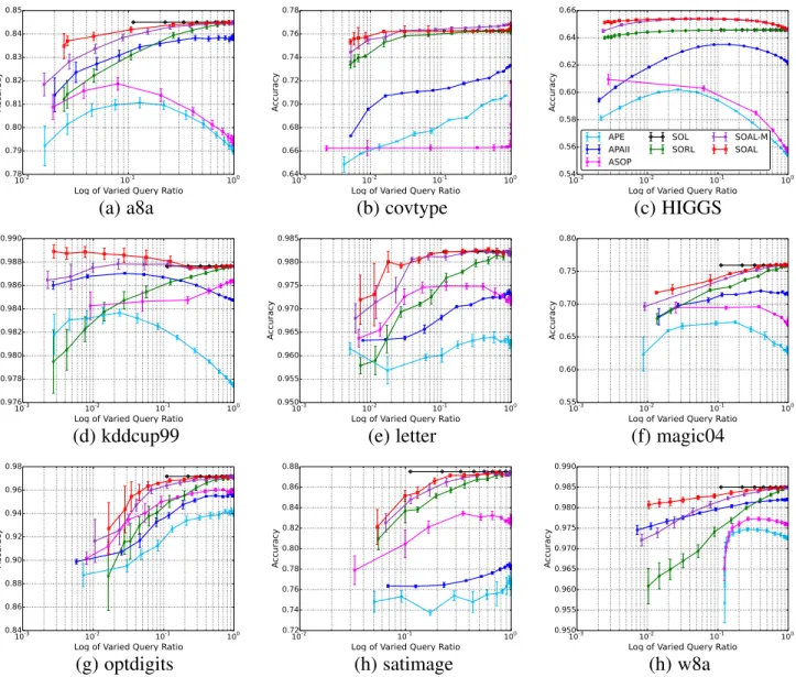
δto different value. Fig. 1 summarizes the average performance on different datasets in terms of accuracy. Based on the results, we can make several observations.
First, in general, second-order based algorithms (SOAL-M and SOAL) can outperform the first-order based algorithms (APE and APAII). This is consistent with the results found in [32], [33] and confirms the necessity of considering second-order information, such as the co-variance matrix, to improve the predictive perfor-mance. Second-order based Active Perceptron (ASOP) algorithm usually performs better than the first-order based Active Percep-tron (APE) algorithm, which is consistent with the finding in [22]. However, on half of the cases, ASOP algorithm even performs worse than the first-order algorithm APAII, one possible reason is that ASOP is more sensitive to noise.
Second, both the proposed algorithm SOAL and its variant SOAL-M algorithm can consistently achieve better performance than the random query strategy algorithm SORL. This observation indicates that both the margin-based query strategy in SOAL-M and our proposed query strategy in SOAL are effective in identi-fying more informative instances to label thus can greatly reduce the cost in labeling. This also indicates that the random query strategy can not effectively identify the informative instances to train the model.
Third, compared to the margin-based query strategy in SOAL-M, our proposed strategy in SOAL can consistently achieve the highest accuracy with varied query ratio on all of the datasets. The reason is that we not only consider the margin value of the instance, but also consider the confidence of model. This makes SOAL can identify the instances on which the model has low uncertainty on its predication and low confidence on the learned classifier, such as in the early rounds of online learning. Besides, we observe that the SOAL can achieve comparable performance as SOL by querying less than 20% of the instances. It should be noted that SOL is a fully-supervised online learning algorithm which uses100%of the query ratio, to make the algorithm clear, we draw a straight line in the Fig. 1.
Last, on some datasets, for example,HIGGSandkddcup99the active learning algorithms SOAL even can outperform the fully-supervised algorithm SOL. We guess that these datasets might contain many noisy labels. It also should be noted that ASOP algorithm performs worse when the query ratio increases on some datasets, such asa8a,HIGGSandmagic04. One possible reason is that ASOP algorithm may suffer the overfitting issue on these datasets.
5.3 Evaluation of Parameter Sensitivity
In the previous section, the parameters η and γ in SOAL are searched from 10[−5:5] via cross validation. In this section, we
evaluate the sensitivity of algorithms to these parameters. Fig. 2 shows the experiment results on a8a, covtype and
HIGGSdatasets. For each dataset, x-axis and y-axis correspond to parametersηandγ, respectively, and different colour corresponds to different performance in terms of accuracy. From the figure, we can observe that parameter η should be neither too small or too large whenγ is fixed. This is consistent with our theoretical analysis in Theorem 1. When η is too small, the second term in Theorem 1 will become the dominant term and thus the performance decreases. When η is too large, the third term in Theorem 1 will become dominant and thus make the performance worse. Typically,ηshould be searched around 1.
In Fig. 2, we can also observe that parameter γ should be decreased when η increases in order to achieve a high accuracy (yellow colour). This observation is also consistent with the theoretical analysis in Theorem 1. When keeping the other terms fixed, we can roughly getγ∼ 1
η2 relationship betweenγandη. In practice, we can either adopt a grid search for both the η
andγor find the bestηfirst followed by searching bestγaround
1
η2.
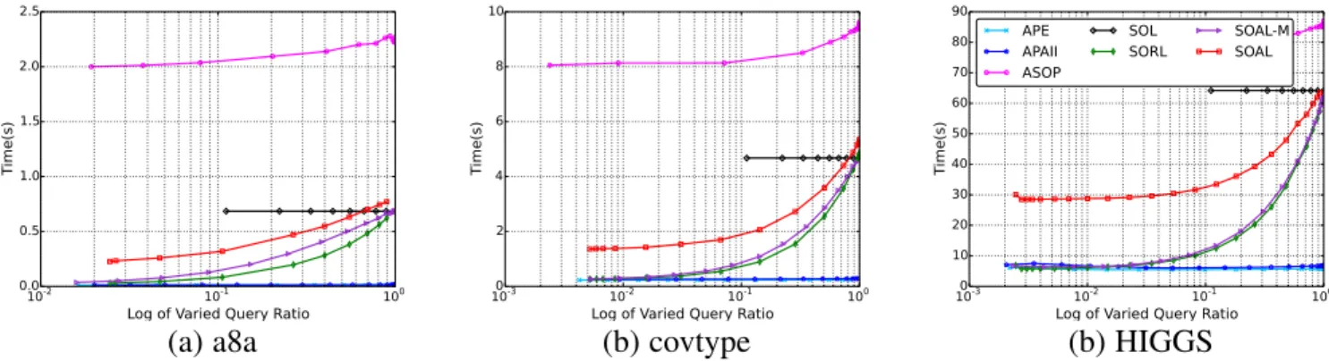
5.4 Evaluation of Scalability and Efficiency
Time complexity is usually a major concern for large-scale prob-lems. To evaluate the scalability of the proposed algorithm SOAL, we conducted this experiment to show the time cost corresponding to the log of varied query ratio on three datasets in Fig. 3. Similar observations also could be made on the other datasets.
First, as expected, the first-order based algorithms APE and APAII are the most efficient ones among all algorithms, which only cost less than 0.5 seconds when being trained on all of the instances. This confirms that the first-order online learning scheme is efficient and easy to be scalable to large scale applications. And we also observe that the second-order based algorithms (ASOP, SOL, SORL, SOAL-M and SOAL) typically cost more time due to the computation of the second-order information Σ. Among them, AOSP usually requires more time, which is almost two times of the other second-order algorithms (SOL, SORL, SOAL-M and SOAL). Moreover, the proposed algorithm SOAL costs more time than its random variant SORL and the margin-based SORL-M algorithms due to the computation of the query strategy shown in Equation 8.
Second, compared to the passive version SOL, the time complexity of both the random algorithm (SORL) and active algorithms (SOAL-M and SOAL) is smaller when query ratio is less than 100%. The reason is that we will skip updating the model if the label of an instance is not queried. When query ratio increases, the time cost of these algorithms slowly converges to the SOL as expected. This indicates that the proposed algorithm
10-2 10-1
100 Log of Varied Query Ratio
0.78 0.79 0.80 0.81 0.82 0.83 0.84 0.85 A ccuracy 10-3 10-2 10-1 100 Log of Varied Query Ratio
0.64 0.66 0.68 0.70 0.72 0.74 0.76 0.78 A ccuracy 10-3 10-2 10-1 100
Log of Varied Query Ratio
0.54 0.56 0.58 0.60 0.62 0.64 0.66 A ccuracy APE APAII ASOP SOL SORL SOAL-M SOAL
(a) a8a
(b) covtype
(c) HIGGS
10-3 10-2 10-1
100
Log of Varied Query Ratio 0.976 0.978 0.980 0.982 0.984 0.986 0.988 0.990 A ccuracy 10-3 10-2 10-1 100 Log of Varied Query Ratio
0.950 0.955 0.960 0.965 0.970 0.975 0.980 0.985 A ccuracy 10-3 10-2 10-1 100
Log of Varied Query Ratio 0.55 0.60 0.65 0.70 0.75 0.80 A ccuracy
(d) kddcup99
(e) letter
(f) magic04
10-3 10-2 10-1
100
Log of Varied Query Ratio 0.84 0.86 0.88 0.90 0.92 0.94 0.96 0.98 A ccuracy 10-2 10-1 100
Log of Varied Query Ratio 0.72 0.74 0.76 0.78 0.80 0.82 0.84 0.86 0.88 A ccuracy 10-3 10-2 10-1 100 Log of Varied Query Ratio
0.950 0.955 0.960 0.965 0.970 0.975 0.980 0.985 0.990 A ccuracy
(g) optdigits
(h) satimage
(h) w8a
Fig. 1: Evaluation of accuracy with respect to log of varied query ratio.
η 10-5 100 105 γ 10-5 100 105 0.76 0.77 0.78 0.79 0.8 0.81 0.82 0.83 0.84 η 10-5 100 105 γ 10-5 100 105 0.6 0.65 0.7 0.75 10−5 100 105 10−5 100 105 η γ 0.61 0.615 0.62 0.625 0.63 0.635 0.64 0.645
(a) a8a
(b) covtype
(b) HIGGS
10-2 10-1 100
Log of Varied Query Ratio 0.0 0.5 1.0 1.5 2.0 2.5 T ime(s) 10-3 10-2 10-1 100
Log of Varied Query Ratio 0 2 4 6 8 10 T ime(s) 10-3 10-2 10-1 100
Log of Varied Query Ratio 0 10 20 30 40 50 60 70 80 90 T ime(s) APE APAII ASOP SOL SORL SOAL-M SOAL
(a) a8a
(b) covtype
(b) HIGGS
Fig. 3: Evaluation of time cost (seconds) with respect to log of varied query ratio.
SOAL can not only reduce the labeling cost shown in Fig. 1, but also speed up the training process by updating the model only with the queried instance.
Third, when query ratio is around 100%, the time cost of SOAL exceeds the one of SOL as SOAL needs extra time to compute the query strategy. However, the extra time cost could be almost ignored considering the high efficiency of the online learning scheme.
5.5 Application on Malicious Web Classification
In this section, we evaluate the proposed Cost-sensitive Second-order Online Active Learning algorithm (SOALCS) shown in
Algorithm 2. To examine its performance, we conduct experiments on two large-scale benchmark datasets for malicious detection problem as follows:
1) “URL” [51]: the task in URL dataset is to classify the malicious URLs from the normal ones. The features in each URL are composed by two parts: (a) Lexical features, the textual properties of the URL itself (not the content of the page), such as length of the hostname, the length of the entire URL, the number of the dots in the URL and so on; (b) Host-based features, such as the IP address properties, WHOIS properties, domain name properties, Geographic properties and so on. In the end, each URL is described by3231961
features.
2) “webspam” [52]: this dataset is taken from a subset of the one used in Pascal Large Scale Learning Challenge. The web spam pages are obtained by extract the URLs from the email spam corpora SpamArchive3. The normal web pages are extracted by traversing the well-known websites, such as news, sports and so on. For each instance, we treat continuous
1bytes as a word, and use word count as the feature value. In the end, we obtain254features for each website. It should be noted that the original URL and webspam datasets were created in purpose to make them somehow balanced, in which the number of malicious samples is roughly similar to the number of normal ones. In the following experiments, we sample two subsets of these two datasets in order to make them more realistic, in which we randomly sample instances to make sure that the ration between the number of positive instances and the number of negative instances equals to the number shown in the table. Table 2 shows the details of these two subsets, in which
3. ftp://spamarchiev.org/pub/archieves
Tp/Tndenotes the ratio of number of malicious samples over the
number of normal ones.
TABLE 2: Summary of the datasets
Dataset #Instances #F eatures Tp/Tn
URL 1,620,187 3,231,961 1:99
webspam 140,000 254 1:63
Based on previous evaluation, we know that the proposed algorithm SOAL can consistently achieve the best performance in terms of accuracy, thus here we only consider the SOAL among the algorithms which adopt the accuracy as evaluation metric. Besides, we also consider the following state-of-the-art cost-sensitive algorithms:
• CSOAL [2]: the state-of-the-art first-order based Cost-sensitive Online Active Learning algorithm, which adopts the margin-based query strategy [7], [22] to decide when to query the instance;
• ARCSOGD [48]: the state-of-the-art second-order based Cost-sensitive fully-supervised Online Learning algorithm, which queries all of the instances for labels;
• SOAL-MCS: a variant of SOALCSalgorithm which adopts
the margin-based query strategy [7], [22] and the cost-sensitive loss function defined in Eq. (12);
• SORLCS: a variant of SOALCSalgorithm which adopts the
random query strategy;
• SOALCS: our proposed Cost-sensitive Second-order based
Online Active Learning method shown in Algorithm 2, which adopts the query strategy shown in Section3.2.2to decide when to query the instance and the cost-sensitive loss defined in Eq. 12.
To make a fair comparison, all algorithms adopt the same experimental setup. For the evaluation metric sum, we set
αp = αn = 0.5 for all cost-sensitive algorithms, while for
cost, we set cp = 0.9 and cn = 0.1. The parameter C in
CSOAL, parametersηandγinARCSOGD, SOALCS,
SOAL-MCS, SORLCSand SOAL are selected by cross validation from [10−5,10−4, . . . ,105]for each dataset. The smoothing parameter δin CSOAL, SOAL-MCS and SOALCS is set as2[−10:2:10] in
order to achieve varied querying ratio.
All the experiments are conducted over 10random permuta-tions on each dataset. The results are reported by averaging over these10runs. We evaluate the online classification performance by three metrics: the accuracy which treats the positives and the
10-4 10-3 10-2 10-1 100 Varied Query Ratio
0.982 0.984 0.986 0.988 0.990 0.992 0.994 0.996 0.998 Accuracy SOAL CSOAL CSAROGD SOAL-MCS SORLCS SOALCS 10-4 10-3 10-2 10-1 100 Varied Query Ratio
0.5 0.6 0.7 0.8 0.9 Sum SOAL CSOAL CSAROGD SOAL-MCS SORLCS SOALCS 10-4 10-3 10-2 10-1 100 Varied Query Ratio
0 2000 4000 6000 8000 10000 12000 14000 16000 Cost SOAL CSOAL CSAROGD SOAL-MCS SORLCS SOALCS
(a) Accuracy
(b) Sum
(b) Cost
Fig. 4: Evaluation of Accuracy, Sum, Cost against the varied query ratios onURLdataset.
10-3 10-2 10-1 100 Varied Query Ratio
0.965 0.970 0.975 0.980 0.985 0.990 0.995 Accuracy SOAL CSOAL CSAROGD SOAL-MCS SORLCS SOALCS 10-3 10-2 10-1 100 Varied Query Ratio
0.45 0.50 0.55 0.60 0.65 0.70 0.75 0.80 Sum SOAL CSOAL CSAROGD SOAL-MCS SORLCS SOALCS 10-3 10-2 10-1 100 Varied Query Ratio
800 1000 1200 1400 1600 1800 2000 2200 Cost SOAL CSOAL CSAROGD SOAL-MCS SORLCS SOALCS
(a) Accuracy
(b) Sum
(b) Cost
Fig. 5: Evaluation of Accuracy, Sum, Cost against the varied query ratios onwebspamdataset.
negatives equally, the weightedsumdefined in Eq. 9 and thecost
defined in Eq. 10.
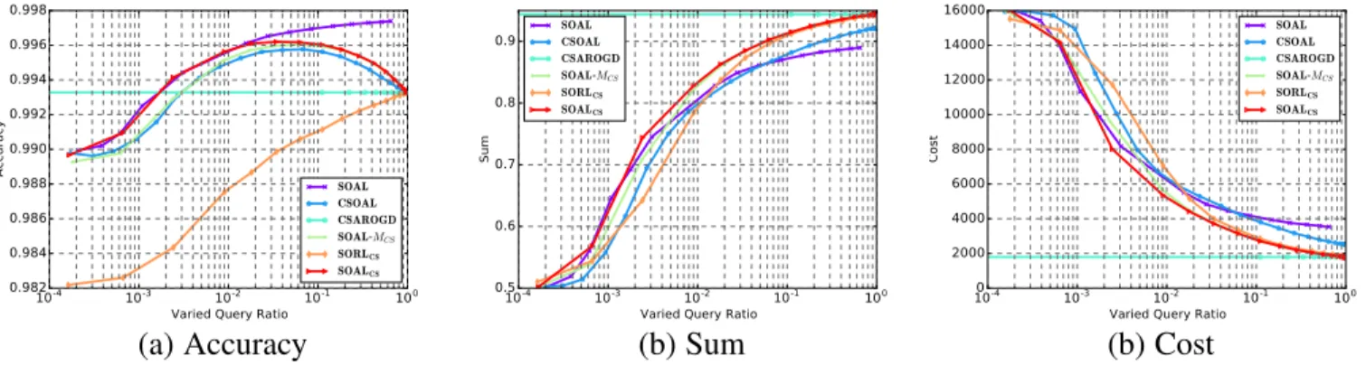
By varying the δ value, we can achieve the performance of algorithm with different query ration. Fig. 4 and Fig. 5 show the results on datasetsURLandwebspam, respectively. As the feature dimension of “URL” is too high to run the experiments in a single PC, so second-order algorithms shown in Fig. 4 are their diagonal versions with updating rule as describe in Eq. (15) and Eq. (16). Based on the results, we can make several observations.
First, we observe that when we aim to achieve best accu-racy shown in Fig. 4 (a) and Fig. 5 (a), the proposed algo-rithm SOAL which adopts regular hinge loss can achieve the best performance. When the query ratio is small, the proposed cost-sensitive algorithm SOALCS can roughly achieve similar
accuracy with the SOAL algorithm. However, when the query ratio increases, the performance of SOAL algorithm consistently increases and achieves the best performance lastly. This indicates that the accuracy in the imbalanced dataset could be a misleading evaluation metric. Thus, this motivates us to investigate the other proper metrics, such assumandcost. It should also be noted that the proposed SOALCSalgorithm can consistently outperform the
other cost-sensitive algorithms even with accuracy as evaluation metric, which again validates the query strategy proposed in Section 3.2.2 is effective in querying informative instances.
Second, when we adopt the evaluation metricsumof sensitiv-ity and specificsensitiv-ity shown in Fig. 4 (b) and Fig. 5 (b), we observe that cost-sensitive algorithm SOALCS, SORLCS can achieve
better performance than SOAL when the query ratio is larger than
1%. It should also be noted that first-order based cost-sensitive
algorithm CSOAL also can outperform SOAL when query ratio is larger than 10%. These observations indicate that it’s necessary to import cost-sensitive strategy which put a larger weight on the malicious samples. Furthermore, it can be observed that the second-order cost-sensitive algorithms SOALCS, SORLCS and
ARCSOGD can outperform the first-order algorithm CSOAL. This indicates its effectiveness to consider the second-order in-formation when designing learning models. We also observe that the proposed algorithm SOALCS can consistently outperform
the margin-based algorithm SOAL-MCS and the random version
SORLCS. This again verifies the effectiveness of the proposed
active learning strategy.
Third, similar observations with metric cost can be made in Fig.4 (c) and Fig. 5 (c) as the metric sum. Besides, it should be noted that the fully-supervised cost-sensitive algorithm ARC-SOGD can achieve the best performance in terms of both sum
and cost, however, ARCSOGD requires to query 100% of the instances, which is costly and time consuming. For example, in the
URLdataset, we have more than1.5million instances and labeling all of these instances would be extreme costly. Our proposed active learning algorithm SOALCScan achieve comparable performance
as ARCSOGD with less than50%query ratio.
6
CONCLUSION
This paper proposed SOAL — a framework of Second-order Online Active Learning in order to address the open challenge of real-life online learning from unlabeled data streams given limited label query budget. By adopting an effective second-order online
learning framework, we proposed to build an effective label query strategy by carefully considering not only the prediction margin of an incoming unlabeled instance but also the confidence of the learner. To further tackle the cost-sensitive learning problems for class-imbalanced applications such as malicious web detection, we extended the SOAL framework by proposing a new cost-sensitive and second-order online active learning algorithm SOALCS to
explicitly optimize the cost-sensitive metrics. We theoretically analyzed the mistake bounds of the proposed SOAL algorithm and conducted a set of extensive experiments to examine its empir-ical effectiveness in terms of accuracy, parameter sensitivity and scalability. We also successfully applied the proposed SOALCS
algorithm to two large-scale malicious web classification tasks. The experimental results showed that our algorithms consistently outperform several state-of-the-art approaches. Future work will explore some hyper-parameter learning strategy for automatically re-adjusting the parametersγandηin the online learning process, and active learning in the transfer learning domain [53], multi-task learning [54] etc.
ACKNOWLEDGMENTS
Steven C.H. Hoi and Chunyan Miao are supported by the National Research Foundation, Prime Ministers Office, Singapore under its International Research Centres in Singapore Funding Initiative.
APPENDIX
PROOF OF
THEOREM
1
To facilitate the proof, we first present a lemma as follows.
Lemma 1. Let (x1, y1), . . . ,(xT, yT) be a sequence of input
examples, where xt ∈ Rd andyt ∈ {−1,+1} for all t. If the
SOAL algorithm is run on this sequence of examples, then the following bound holds for anyw∈Rd,
Zt Mt(δ+|pt|) +Lt(δ− |pt|) ≤ 1 2ηZt kµt−δµk2Σ−1 t+1 − kµt+1−δµk2Σ−1 t+1 +kµt−µt+1k2Σ−1 t+1 +δ`t(µ) , whereδ >0.
Proof. When Zt = 0, it is easy to verify the inequality in the
theorem, using the fact`t≥0.
WhenZt= 1, it is easy to observe that
µt+1= arg min µ ht(µ) ht(µ) = 1 2kµt−µk 2 Σ−t+11 +ηg > t µ.
Becausehtis convex, we have the following inequality∀µ, 0≤∂ht(µt+1)>(µ−µt+1)
=
Σ−t+11(µt+1−µt) +ηgt >
(µ−µt+1).
Re-arranging the above inequality will result in
ηg>t(µt+1−µ) ≤µt+1−µt)>Σt−+11(µ−µt+1 =1 2 kµt−µk2 Σ−t+11 − kµt+1−µk 2 Σ−t+11 −1 2 kµt−µt+1k2 Σ−t+11 (17)
Now, we would provide a lower bound forg>
t(µt+1−µ), g>t(µt+1−µ) =g>t(µt−µ) +g>t (µt+1−µt) = (Lt+Mt)(−ytx>tµt) + (Lt+Mt)ytx>tµ −1 ηkµt+1−µtk 2 Σ−t+11, (18)
where the second equality used the factsgt= (Lt+Mt)(−ytxt)
and∂ht(µt+1) = 0i.e.,
Σ−t+11(µt+1−µt) +ηgt= 0. (19)
Combining the above equality (18) with the facts
Mt(−ytx>tµt) =Mt|ytx>tµt|=Mt|pt|
Lt(−ytx>tµt) =Lt(−|ytx>t µt|) =−Lt|pt|
ytx>tµ+δ`t(µ/δ)≥ytx>tµ+δ(1−ytx>tµ/δ) =δ,
we get the following bound forg>t(µt+1−µ),
g>t(µt+1−µ) ≥(Mt|pt| −Lt|pt|) + (Lt+Mt)[δ−δ`t(µ/δ)] −1 ηkµt+1−µtk 2 Σ−t+11 = [Mt(δ+|pt|) +Lt(δ− |pt|)]− 1 ηkµt+1−µtk 2 Σ−1 t+1 −(Lt+Mt)δ`t(µ/δ). (20)
Combining the above two inequalities (17) and (20), will give the following important inequality
[Mt(δ+|pt|) +Lt(δ− |pt|)] ≤ 1 2η kµt−µk2 Σ−t+11 − kµt+1−µk 2 Σ−t+11 − kµt−µt+1k 2 Σ−t+11 +1 ηkµt+1−µtk 2 Σ−t+11 +δ`t(µ/δ) = 1 2η kµt−µk2Σ−1 t+1 − kµt+1−µk2Σ−1 t+1 +kµt−µt+1k2Σ−1 t+1 +δ`t(µ/δ)
Replacingµwithδµconcludes the proof. We now proof the proposed Theorem 1 as follows.
Proof. Firstly, according to the equality (19), we have
kµt−µt+1k2 Σ−t+11 =η2g>tΣt+1gt =η2(Mt+Lt)x>tΣt+1xt =η2(Mt+Lt) x>tΣtxt− x>t Σtxtx>tΣtxt γ+x>t Σtxt =η2(Mt+Lt) γvt γ+vt ,
where we used the updating rule of Σ. Plugging it into the inequality in the Lemma 1 and re-arranging it will give
Zt Mt δ+|pt| − ηγvt 2(γ+vt) +Lt δ− |pt| − ηγvt 2(γ+vt) ≤ 1 2ηZt h kµt−δµk2Σ−1 t+1 − kµt+1−δµk2Σ−1 t+1 i +δ`t(µ)
Summing the above inequality overt= 1,2, . . . , T and using the definition ofρtcan give
T X t=1 Zt Mt(δ+ρt) +Lt(δ+ρt−2|pt|) ≤ 1 2η T X t=1 Zt kµt−δµk2 Σ−1 t+1 − kµt+1−δµk2 Σ−1 t+1 +δ T X t=1 Zt`t(µ) (21)
Now, we would like to bound the right-hand side of the above inequality. Firstly, we bound the first term as
T X t=1 Zt h kµt−δµk2 Σ−t+11 − kµt+1−δµk 2 Σ−t+11 i ≤ kµ1−δµk2 Σ−21+ T X t=2 h kµt−δµk2 Σ−t+11 − kµt−δµk 2 Σ−t1 i ≤ kµ1−δµk2Tr(Σ−1 2 ) + T X t=2 kµt−δµk2Tr(Σ−1 t+1−Σ −1 t ) = max t≤T kµt−δµk 2TrΣ−1 T+1 ≤2(Dµ+ (1−δ)2kµk2)Tr(Σ−T1+1) (22) where Dµ = maxt≤Tkµt−µk2. Plugging the above upper
bound (22) into the inequality (21), we can get
T X t=1 Zt[Mt(δ+ρt) +Lt(δ+ρt−2|pt|)] ≤ 1 η Dµ+ (1−δ) 2kµk2 TrΣ−T+11 +δ T X t=1 Zt`t(µ) (23)
Whenρt>0, usingEtZt=δ/(δ+ρt), we have
E Zt[Mt(δ+ρt) +Lt(δ+ρt−2|pt|)] =δE[Mt] +δE[Lt(1−2|pt|/(δ+ρt))] ≥δE[Mt] + (δ−2)E[Lt]. Whenρt≤0, i.e.,|pt| ≤ 2(ηγvγ+vt t), usingEtZt= 1, we have E Zt[Mt(δ+ρt) +Lt(δ+ρt−2|pt|)] ≥EMt δ− ηγvt 2(γ+vt) +ELt δ− ηγvt γ+vt To summarize, T X t=1 E Zt[Mt(δ+ρt) +Lt(δ+ρt−2|pt|)] ≥δE " T X t=1 Mt # +δE " T X t=1 Lt # −2E X ρt>0 Lt −E X ρt<0 Mt ηγvt 2(γ+vt) −E X ρt<0 Lt ηγvt γ+vt
Taking expectation of the inequality (23) and combining with the above inequality conclude the proof.
REFERENCES
[1] T. Yang, M. Mahdavi, R. Jin, and S. Zhu, “Regret bounded by gradual variation for online convex optimization,”Machine Learning, Oct. 2013. [2] P. Zhao and S. C. Hoi, “Cost-sensitive online active learning with application to malicious url detection,” inProceedings of the 19thACM
SIGKDD international conference on Knowledge discovery and data mining - KDD ’13, (New York, New York, USA), p. 919, ACM Press, 2013.
[3] H. B. Ammar, U. EDU, E. Eaton, P. Ruvolo, O. EDU, M. E. Taylor, and W. EDU, “Online multi-task learning for policy gradient methods,”
ICML 2014, 2014.
[4] C. Zhang, P. Zhao, S. Hao, Y. C. Soh, and B. S. Lee, “Rom: A robust online multi-task learning approach,” in2016 IEEE 16th International Conference on Data Mining (ICDM’16),, pp. 1341–1346, IEEE, 2016. [5] C. C. Cao, L. Chen, and H. V. Jagadish, “From labor to trader: Opinion
elicitation via online crowds as a market,” inProceedings of the 20th
ACM SIGKDD International Conference on Knowledge Discovery and Data Mining, KDD ’14, (New York, NY, USA), pp. 1067–1076, ACM, 2014.
[6] G. Li, S. C. Hoi, K. Chang, W. Liu, and R. Jain, “Collaborative online multitask learning,”Knowledge and Data Engineering, IEEE Transac-tions on, vol. 26, no. 8, pp. 1866–1876, 2014.
[7] J. Lu, Z. Peilin, and C. S. Hoi, “Online passive aggressive active learning and its applications,”Machine Learning, vol. 103(2), pp. 141–183, 2016. [8] D. Sahoo, S. C. Hoi, and B. Li, “Online multiple kernel regression,” inProceedings of the 20thACM SIGKDD international conference on
Knowledge discovery and data mining, pp. 293–302, ACM, 2014. [9] S. Hao, P. Zhao, Y. Liu, S. C. H. Hoi, and C. Miao, “Online multi-task
relative similarity learning,” inThe 26th International Joint Conference on Artificial Intelligence (IJCAI’17), 2017.
[10] S. C. Hoi, J. Wang, and P. Zhao, “LIBOL: a library for online learning algorithms,” Journal of Machine Learning Research, vol. 15, no. 1, pp. 495–499, 2014.
[11] P. Ruvolo and E. Eaton, “Online multi-task learning via sparse dictionary optimization,” inProceedings of the Twenty-Eighth AAAI Conference on Artificial Intelligence, July 27 -31, 2014, Qu´ebec City, Qu´ebec, Canada.
(C. E. Brodley and P. Stone, eds.), pp. 2062–2068, AAAI Press, 2014. [12] M. Aleksandrov, H. Aziz, S. Gaspers, and T. Walsh, “Online fair division:
Analysing a food bank problem,” inProceedings of the Twenty-Fourth International Joint Conference on Artificial Intelligence, IJCAI 2015, Buenos Aires, Argentina, July 25-31, 2015(Q. Yang and M. Wooldridge, eds.), pp. 2540–2546, AAAI Press, 2015.
[13] X. Guo, “Online robust low rank matrix recovery,” inProceedings of the Twenty-Fourth International Joint Conference on Artificial Intelligence, IJCAI 2015, Buenos Aires, Argentina, July 25-31, 2015(Q. Yang and M. Wooldridge, eds.), pp. 3540–3546, AAAI Press, 2015.
[14] K. Hayakawa, E. H. Gerding, S. Stein, and T. Shiga, “Online mechanisms for charging electric vehicles in settings with varying marginal electricity costs,” inProceedings of the Twenty-Fourth International Joint Confer-ence on Artificial IntelligConfer-ence, IJCAI 2015, Buenos Aires, Argentina, July 25-31, 2015(Q. Yang and M. Wooldridge, eds.), pp. 2610–2616, AAAI Press, 2015.
[15] F. Jahedpari, “Artificial prediction markets for online prediction,” in
Proceedings of the Twenty-Fourth International Joint Conference on Artificial Intelligence, IJCAI 2015, Buenos Aires, Argentina, July 25-31, 2015(Q. Yang and M. Wooldridge, eds.), pp. 4371–4372, AAAI Press, 2015.
[16] J. Veness, M. Hutter, L. Orseau, and M. G. Bellemare, “Online learning of k-cnf boolean functions,” inProceedings of the Twenty-Fourth Inter-national Joint Conference on Artificial Intelligence, IJCAI 2015, Buenos Aires, Argentina, July 25-31, 2015(Q. Yang and M. Wooldridge, eds.), pp. 3865–3873, AAAI Press, 2015.
[17] J. Wan, P. Wu, S. C. H. Hoi, P. Zhao, X. Gao, D. Wang, Y. Zhang, and J. Li, “Online learning to rank for content-based image retrieval,” inProceedings of the Twenty-Fourth International Joint Conference on Artificial Intelligence, IJCAI 2015, Buenos Aires, Argentina, July 25-31, 2015(Q. Yang and M. Wooldridge, eds.), pp. 2284–2290, AAAI Press, 2015.
[18] B. Wang and J. Pineau, “Online boosting algorithms for anytime transfer and multitask learning,” inTwenty-Ninth AAAI Conference on Artificial Intelligence, 2015.
[19] B. Settles, “Active learning,”Synthesis Lectures on Artificial Intelligence and Machine Learning, vol. 6, pp. 1–114, June 2010.
[20] S. Tong,Active learning: theory and applications. PhD thesis, Stanford University, 2001.
[21] S. Hanneke, “Theory of disagreement-based active learning,” Founda-tions and TrendsR in Machine Learning, vol. 7, no. 2-3, pp. 131–309, 2014.
[22] N. Cesa-Bianchi, C. Gentile, and L. Zaniboni, “Worst-case analysis of selective sampling for linear classification,” The Journal of Machine Learning Research, vol. 7, pp. 1205–1230, Dec. 2006.
[23] N. Cesa-Bianchi, C. Gentile, and L. Zaniboni, “Worst-case analysis of selective sampling for linear-threshold algorithms,” inAdvances in Neural Information Processing Systems 17 [Neural Information Pro-cessing Systems, NIPS 2004, December 13-18, 2004, Vancouver, British Columbia, Canada], pp. 241–248, 2004.
[24] D. Sahoo, C. Liu, and S. C. Hoi, “Malicious url detection using machine learning: A survey,”arXiv preprint arXiv:1701.07179, 2017.
[25] S. Hao, P. Zhao, J. Lu, S. C. Hoi, C. Miao, and C. Zhang, “Soal: Second-order online active learning,” inData Mining (ICDM), 2016 IEEE 16th International Conference on, pp. 931–936, IEEE, 2016.
[26] P. Zhao, R. Jin, T. Yang, and S. C. Hoi, “Online auc maximization,” in
Proceedings of the 28th international conference on machine learning (ICML-11), pp. 233–240, 2011.
[27] H. Block, “The perceptron: A model for brain functioning. i,”Reviews of Modern Physics, vol. 34, no. 1, 1962.
[28] M. Mohri and A. Rostamizadeh, “Perceptron mistake bounds,”arXiv preprint arXiv:1305.0208, 2013.
[29] Y. Li and P. M. Long, “The relaxed online maximum margin algorithm,”
Machine Learning, vol. 46, no. 1-3, pp. 361–387, 2002.
[30] K. Crammer, O. Dekel, J. Keshet, and S. Shalev-shwartz, “Online passive-aggressive algorithms,”The Journal of Machine Learning, vol. 7, pp. 551–585, 2006.
[31] N. Cesa-Bianchi, A. Conconi, and C. Gentile, “A second-order percep-tron algorithm,”SIAM Journal on Computing, vol. 34, pp. 640–668, Jan. 2005.
[32] M. Dredze, K. Crammer, and F. Pereira, “Confidence-weighted linear classification,” in Proceedings of the 25th international conference on Machine learning, pp. 264–271, ACM, 2008.
[33] K. Crammer, A. Kulesza, and M. Dredze, “Adaptive regularization of weight vectors,”Machine Learning, vol. 91, pp. 155–187, Mar. 2013. [34] J. Wang, P. Zhao, and S. C. Hoi, “Exact soft confidence-weighted
learn-ing,” inProceedings of the 29th International Conference on Machine Learning (ICML-12)(J. Langford and J. Pineau, eds.), (New York, NY, USA), pp. 121–128, ACM, 2012.
[35] S. Tong and D. Koller, “Support vector machine active learning with applications to text classification,” The Journal of Machine Learning Research, pp. 45–66, 2002.
[36] Y. Freund and Y. Mansour, “Learning under persistent drift,” in Compu-tational Learning Theory, pp. 109–118, 1997.
[37] S. Hanneke and L. Yang, “Minimax analysis of active learning,”Journal of Machine Learning Research, vol. 16, pp. 3487–3602, 2015. [38] S. Hanneke, “The optimal sample complexity of pac learning,”Journal
of Machine Learning Research, vol. 17, no. 38, pp. 1–15, 2016. [39] Y. Guo and D. Schuurmans, “Discriminative batch mode active learning,”
in Advances in neural information processing systems, pp. 593–600, 2008.
[40] V. S. Sheng, F. Provost, and P. G. Ipeirotis, “Get another label? improving data quality and data mining using multiple, noisy labelers,” in Proceed-ings of the 14th ACM SIGKDD international conference on Knowledge discovery and data mining, pp. 614–622, ACM, 2008.
[41] S. Hanneke, “Activized learning : Transforming passive to active with improved label complexity∗,”Journal of Machine Learning Research, vol. 13, pp. 1469–1587, 2012.
[42] K. Fujii and H. Kashima, “Budgeted stream-based active learning via adaptive submodular maximization,” inAdvances in Neural Information Processing Systems 29 (D. D. Lee, M. Sugiyama, U. V. Luxburg, I. Guyon, and R. Garnett, eds.), pp. 514–522, Curran Associates, Inc., 2016.
[43] K. H. Brodersen, C. S. Ong, K. E. Stephan, and J. M. Buhmann, “The balanced accuracy and its posterior distribution,” inPattern recognition (ICPR), 2010 20th international conference on, pp. 3121–3124, IEEE, 2010.
[44] R. Akbani, S. Kwek, and N. Japkowicz, “Applying support vector machines to imbalanced datasets,” inEuropean conference on machine learning, pp. 39–50, Springer, 2004.
[45] M. Tan, “Cost-sensitive learning of classification knowledge and its applications in robotics,”Machine Learning, vol. 13, no. 1, pp. 7–33, 1993.
[46] A. C. Lozano and N. Abe, “Multi-class cost-sensitive boosting with p-norm loss functions,” inProceedings of the 14th ACM SIGKDD