Application of Synthetic Informative Minority Over-Sampling (SIMO) Algorithm Leveraging Support Vector Machine (SVM) On Small Datasets with Class Imbalance

(1)

Technological University Dublin Technological University Dublin

ARROW@TU Dublin

Dissertations School of Computing

2018

Application of Synthetic Informative Minority Over-Sampling

(SIMO) Algorithm Leveraging Support Vector Machine (SVM) On

Small Datasets with Class Imbalance

Akshatha Fakkeriah Kallappanamatt Technological University Dublin, Ireland

Follow this and additional works at: https://arrow.tudublin.ie/scschcomdis Part of the Computer Engineering Commons

Recommended Citation Recommended Citation

Fakkeriah Kallappanamatt, A. Application of Synthetic Informative Minority Over-Sampling (SIMO) Algorithm Leveraging Support Vector Machine (SVM) On Small Datasets with Class Imbalance. M.Sc. in Computing (Data Analytics), DIT, 2018.

This Dissertation is brought to you for free and open access by the School of Computing at ARROW@TU Dublin. It has been accepted for inclusion in Dissertations by an authorized administrator of ARROW@TU Dublin. For more information, please contact

[email protected], [email protected], [email protected].

This work is licensed under a Creative Commons Attribution-Noncommercial-Share Alike 3.0 License

(2)

Application of Synthetic Informative Minority

Over-Sampling (SIMO) Algorithm Leveraging Support Vector

Machine (SVM) On Small Datasets with Class Imbalance

Akshatha Fakkeriah Kallappanamatt

A dissertation submitted in partial fulfilment of the requirements of

Dublin Institute of Technology for the degree of

M.Sc. in Computing (Data Analytics)

(3)

i

DECLARATION

I certify that this dissertation which I now submit for examination for the award of MSc in Computing (Data Analytics), is entirely my own work and has not been taken from the work of others save and to the extent that such work has been cited and acknowledged within the test of my work.

This dissertation was prepared according to the regulations for postgraduate study of the Dublin Institute of Technology and has not been submitted in whole or part for an award in any other Institute or University.

The work reported on in this dissertation conforms to the principles and requirements of the Institute’s guidelines for ethics in research.

Signed: Akshatha Fakkeriah Kallappanamatt Date: 04 September 2018

(4)

ii

ABSTRACT

Developing predictive models for classification problems considering imbalanced datasets is one of the basic difficulties in data mining and decision-analytics. A classifier’s performance will decline dramatically when applied to an imbalanced dataset. Standard classifiers such as logistic regression, Support Vector Machine (SVM) are appropriate for balanced training sets whereas provides suboptimal classification results when used on unbalanced dataset. Performance metric with prediction accuracy encourages a bias towards the majority class, while the rare instances remain unknown though the model contributes a high overall precision. There are chances where minority instances might be treated as noise and vice versa. (Haixiang et al., 2017). Wide range of Class Imbalanced learning techniques are introduced to overcome the above-mentioned problems, although each has some advantages and shortcomings.

This paper provides details on the behavior of a novel imbalanced learning technique Synthetic Informative Minority Over-Sampling (SIMO) Algorithm Leveraging Support Vector Machine (SVM) on small datasets of records less than 200. Base classifiers, Logistic regression and SVM is used to validate the impact of SIMO on classifier’s performance in terms of metrices G-mean and Area Under Curve. A Comparison is derived between SIMO and other algorithms SMOTE, Smote-Borderline, ADAYSN to evaluate performance of SIMO over others.

Key words: Class imbalance, Class imbalance learning, Machine learning, Supervised learning, Small datasets.

(5)

iii

ACKNOWLEDGEMENTS

I would like to express my sincere thanks to the supervisor Dr. Luca Longo for his encouragement and support, imparting constructive suggestions and recommendations and guiding me throughout the research project.

I would like to express my regards to one of the author of SIMO algorithm, Professor Saeed Piri for clarifying algorithm related queries when necessary. I would like to thank my classmate Jaydeep for reviewing and helping in translating the algorithm from Matlab code to python.

I would also like to express my gratitude towards all the ‘Dublin Institute of Technology academic staffs’ especially the professors who shared valuable ken and for their help, support and guidance throughout the academic.

(6)

iv

TABLE OF FIGURES

2.1 SMOTE methodology in generating synthetic data points ……….. 9

2.2 Positive instances lie further away from the ideal boundary (horizontal line) than the negative instances. As a result, SVM learns a boundary (slanted line) that is too close to the positive support vectors ………..14

2.3 Block diagram of weighed-SMOTE ………... 18

2.4 (a) features a sparse majority class, a minority class region, and many minority outliers. (b) Cluster-SMOTE detects two clusters of minority points and uses this information to generate new synthetic examples, as shown in (c) ……… 19

3.1 CRISP-DM framework ………... 23

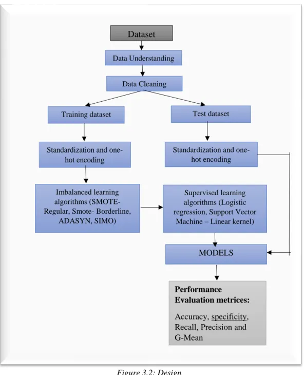
3.2 Design ……… 29

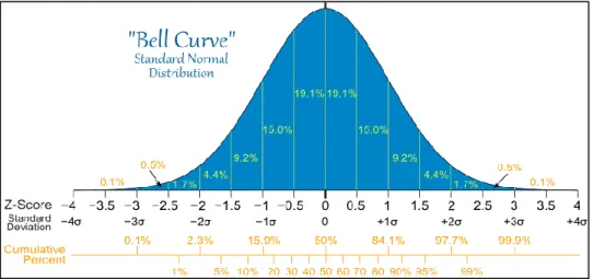
3.3 Bell Curve ………... 31

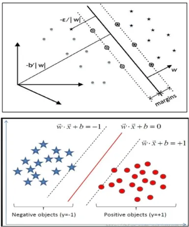
3.5 w is a weight vector, x is input vector and b is the bias ………. 34

3.6 Linear Classification: H1, H2, H3 - Separation hyperplanes. H1 does not separate the two classes; H2 separates but with a very tinny margin between the classes and H3 separates the two classes with much better margin than H2 ...……….. 34

3.7 ROC chart ………... 36

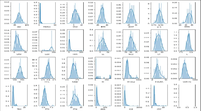
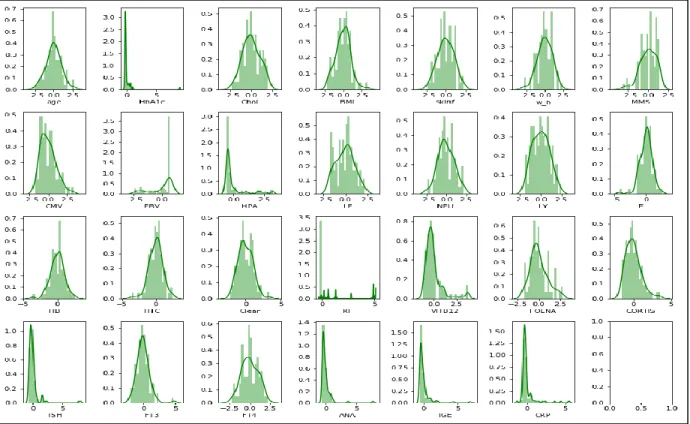
4.1 Histogram plots obtained before Normalization – Normality check ... 42

4.2 Histograms obtained after Normalization - Normality check ………. 42

4.3 Frequency plot - Relation between Categorical and target variable ……… 43

4.4 Histogram plots obtained before Normalization – Normality check ...………… 45

4.5 Histogram plots obtained after Normalization – Normality check ……….. 45

4.6 Frequency plot - Relation between Categorical and target variable ……… 46

4.7 Correlation matrix represented in a heat map ………. 47

4.8 Histogram plots obtained before Normalization – Normality check ... 49

4.9 Histogram plots obtained after Normalization – Normality check ………. 49

4.10 Frequency plot- Relation between Categorical and target variable ... 50

4.11 Correlation matrix represented in a heat map ……… 51

4.13 Missing value analysis report ………..………. 52

4.12 Histogram plots obtained before Normalization – Normality check ………… 52

4.13 Histogram plots obtained after Normalization – Normality check ……… 53

(10)

viii

4.15 Correlation matrix represented in a heat map ………..… 54 4.16 Performance Comparison bar graph: Biomarker – Logistic regression ……... 59 4.17 Performance Comparison bar graph: Biomarker – SVM ……… 59 4.18 Performance Comparison bar graph: Hepatitis – Logistic Regression ...…… 60 4.19 Performance Comparison bar graph: Hepatitis – SVM ..……… 60 4.20 Performance Comparison bar graph: Echocardiogram – Logistic Regression .. 61 4.21 Performance Comparison bar graph: Echocardiogram – SVM ...…... 61 4.22 Performance Comparison bar graph: Immunotherapy – Logistic regression .... 62 4.23 Performance Comparison bar graph: Immunotherapy – SVM ...……… 63

(11)

ix

TABLE OF TABLES

2.1 Safe-level SMOTE decision table ……… 11

3.1 Dataset description ………... 24

3.2 Biomarker dataset, C – Categorical variables, N ……… 25

3.3 Hepatitis dataset, C – Categorical variables, N – Numerical variables ………... 26

3.4 Echocardiogram dataset, C – Categorical variables, N – Numerical variable ……… 27

3.5 Immunotherapy, C – Categorical variables, N – Numerical variables ………… 28

4.1 Descriptive statistics of variables ……… 41

4.2 Descriptive statistics of variables ………... 41

4.3 Descriptive statistics of variables ………....……… 41

4.4 Descriptive statistics of variables ……… 41

4.5 Missing value Analysis report ……… 41

4.6 Descriptive Statistics ……….. 44

4.7 Missing value analysis report ………. 44

4.8 Descriptive statistics ……… 48

4.9 Missing Value Analysis Report ………... 49

4.10 Descriptive statistics ……….. 52

4.11 Missing value analysis report ………... 52

4.12 Details on SIMO parameter settings and the resampled ratio ……….. 56

4.13 Details on SIMO parameter settings and the resampled ratio ………... 56

4.14 Details on SIMO parameter settings and the resampled ratio ……… 56

4.15 Details on SIMO parameter settings and the resampled ratio ……… 57

4.16 Tuning parameters for Logistic regression ………. 58

4.17: Tuning parameters for SVM ………. 58

(12)

x

LIST OF ACRONYMS

AUC Area Under the Curve

CRISP-DM Cross Industry Standard Process for Data Mining

CV Cross Validation

FN False Negative

FP False Positive

TN True Negative

TP True Positive

TPR True Positive Rate

FPR False Positive Rate

SMOTE Synthetic Minority Over-Sampling Technique

SVM Support Vector Machine

TN True Negative

KNN K Nearest Neighbour

SVM Support Vector Machine

ROC Receiver Operating Characteristic

SIMO Synthetic informative minority Oversampling

MSMOTE Modified Synthetic Minority Oversampling

ADASYN Adaptive Synthetic Sampling

ASUWO Adaptive semi-unsupervised weighted oversampling

SUNDO Similarity-based Under Sampling and Normal Distribution-based Oversampling

SMOTE-B1 SMOTE Borderline 1

(13)

1

CHAPTER 1 INTRODUCTION

1.1 Background

Health informatics is defined as “all aspects of understanding and promoting the effective organization, analysis, management, and use of information in health care”. Whereas, Data mining is defined as “a process of nontrivial extraction of implicit, previously unknown and potentially useful information from the data stored in a database”, the core step in the Knowledge discovery in databases (KDD). It is the nontrivial process identifying valid, novel, potentially useful, and ultimately understandable patterns in data. The amalgamation of these two is becoming popular nowadays because with the help of an appropriate computer-based systems and efficient analytical methodologies one can meticulously discover the significant hidden knowledge from huge medical databases which includes finding correlations or patterns among different fields in large medical databases. (Kavakiotis et al., 2018)

Predictive Analytics is nothing but the application of data mining techniques incorporating machine learning algorithms on historic data in predicting the future or the unknown. It is gaining a wide range of importance in various disciplines and healthcare domain is one among them. Machine learning can be formally defined as, A computer program is said to learn from experience E with respect to some class of tasks T and performance measure P, if its performance at tasks in T, as measured by P, improves with experience E. Application of predictive analytics in healthcare domain majorly includes, Prediction of presence or susceptibility of an individual to disease, mortality risks considering different scenarios, survivability of a patient after a medical treatment and so on. (Kavakiotis et al., 2018)

Machine learning is classified into three categories namely Supervised learning, Unsupervised learning and Reinforcement learning. Unsupervised learning draw inferences from unlabeled datasets whereas Supervised learning predicts the unknown with a prior knowledge of the datasets. It uses labelled data. Classification is one of the supervised

(14)

2

learning method which is used to predict the target set which is dichotomous in nature. This can be achieved by available algorithms like Logistic regression, Super Vector Machine, Decision tree, Random forest, etc. (Sharma & Sharma, 2016)

The usual problem faced by classification algorithms that would make its functionality worthless is Class imbalance problem. Standard Classifiers like Logistic regression and SVM works fine on balanced datasets but their performance deteriorates when it comes to working on Imbalanced datasets. Class imbalance is a scenario where the examples of one class significantly outnumbers the other and the branch of machine learning which deals with such problems is named Class Imbalance learning. Recent researches are more focused on imbalanced and overlapping datasets as real data is often skewed like medical diagnosis, oil blowout detection, financial fraud detection, network intrusion detection, spam detection, text classification, etc. Problem of small disjuncts and small sample size with high feature dimensionality causing classification errors are often encountered and these are closely related problems to class imbalance problem.

Imbalance learning algorithm can be categorized into data-level approach and algorithm-level approach. The data-level approach occurs at the pre-processing phase whereas algorithm level is modifying the learning algorithms itself to perform efficiently on imbalanced data. Data-level approach includes Resampling which is again categorized into Oversampling and Under sampling techniques. Oversampling technique is a popular approach especially oversampling by synthetic data generation has gained a huge research importance, popular ones are SMOTE, Borderline-SMOTE, ADASYN. Many approaches have been proposed having its own merits and demerits wherein Oversampling by Synthetic data generation.

The problem of overfitting, overgeneralization of the models, chance of oversampling noise examples which will increase the misclassification rate are few drawbacks which most of the oversampling algorithms come across. To overcome these disadvantages Cost sensitive and Ensemble-based learning techniques are approached. Cost-sensitive methods assigns different costs to the samples of different classes to make minority examples more important during training process. Ensemble learning methods is the combination of ensemble learning algorithms and any of the above-mentioned

(15)

3

approaches. This includes, SMOTEBoost, SMOTEBagging, AdaCost and so on. (Peng, 2015).

1.2 Research Project

The objective of the experiment is to evaluate the performance of novel imbalanced learning technique, Synthetic Informative Minority Over-Sampling (SIMO) Algorithm Leveraging Support Vector Machine (SVM) on small datasets. The performance comparison is carried out with existing imbalance learning techniques like SMOTE, SMOTE-Borderline and ADASYN which are considered as baseline algorithms for this research. Standard Supervised learning algorithms Linear algorithms and SVM is used to assess the impact of SIMO on these classifier’s prediction performance. To obtain optimized results from the classifiers GridsearchCV with five folds is used. Since the experiment involves small datasets of class imbalance problem, performance metrices G mean and Area Under Curve is considered for the evaluation and accuracy is prioritized the least. Five iterations are carried out and the mean G mean and AUC is tabulated to obtain visual representations for easier analysis.

The research question which can be answered from this research is as stated below, “Can performance of the classifiers on small datasets, significantly improve on the application of ‘SIMO leveraging SVM’ over the application of baseline imbalanced learning algorithms?”

**SIMO: Synthetic Informative Minority Over-Sampling **SVM: Support Vector Machine

**Baseline imbalanced learning algorithms: SMOTE, SMOTE-Borderline1, SMOTE- Borderline2 and ADASYN.

(16)

4 1.3 Research Objectives

The key objective of this research is to evaluate the performance of novel imbalanced learning technique, Synthetic Informative Minority Over-Sampling (SIMO) Algorithm Leveraging Support Vector Machine (SVM) on small datasets. To achieve the same four datasets are chosen which belongs to univariate classification problem and following steps are carried out,

1. Data understanding comprising a detailed analysis of the datasets in terms of its distribution through graphs, minimum and maximum values, central tendency and standard deviation of the variables and the relationship they share with the target and themselves.

2. Data cleaning involves removal of missing values and imputation.

3. Data preparation is carried out which includes Standardization (Z-scores), One-hot Encoding.

4. Data partition with a stratified split of 75 percent train data and 25 percent test data.

5. Application of Oversampling techniques SMOTE, SMOTE-Borderline1, SMOTE-Borderline2, ADASYN and SIMO on train data.

6. Resampled or oversampled data is trained using supervised learning algorithms Logistic Regression and SVM.

7. The model results are recorded with respect to G mean, AUC obtained from ROC plots and Accuracy from confusion matrix.

8. Graphical representation is obtained for model’s performance comparison on the application of imbalanced learning algorithms.

9. Use of Wilcoxon Signed rank test to statistically asses the results and determine the rejection or acceptance of research hypothesis that answers research question.

(17)

5 1.4 Research Methodologies

The key focus of this research is to evaluate the impact of novel imbalanced learning technique, Synthetic Informative Minority Over-Sampling (SIMO) Algorithm Leveraging Support Vector Machine (SVM) on classifiers performances for small datasets. Hence, existing datasets which are small in sample size and have moderate to high class imbalance are chosen.

The type of research carried out is Secondary and the methodology involves a systematic empirical investigation of quantitative properties available in the collected information. The results obtained from the experiment will be used as a source of support in rejecting or retaining the hypothesis that will in turn answer the research question.

1.5 Scope and Limitations

The scope of the project is to examine the influence of novel imbalanced learning technique, Synthetic Informative Minority Over-Sampling (SIMO) Algorithm Leveraging Support Vector Machine (SVM) on small datasets. Usually domains like Biomedical and their related fields, health informatics will have small data to analyze and classifiers usually will fail to perform well as there will be no sufficient information available to learn. Small datasets with class imbalance can make classifier even worthless as they tend to misclassify minority examples as majority since majority examples are present in abundance. The current study is focused on similar problem investigating the applicational effect of SIMO on four datasets with small sample size with class imbalance.

Considering only four datasets to evaluate SIMO algorithm is the limitation of this research. Understanding and pre-processing of the datasets of records less than 150 without losing information and treating the class imbalance associated with it is another limitation to overcome.

1.5Document Outline

The Report document includes following section and the contents covered in each section is descripted below.

(18)

6

Chapter 2 (Literature Review) gives an overview of the literatures related to Class Imbalance problem, its impact on classifiers and various learning methods proposed to overcome the limitations. This section also discusses benefits and shortcomings of the proposed methods and how one is efficient than other. It also explains the working of SIMO algorithm, its merits and demerits in detail.

Chapter 3 (Design and Methodology) outlines the design implemented in the research, techniques involved in the design and its purpose, its advantage and limitations, usefulness of its implementation.

Chapter 4 (Results and Discussions) provides an account of results obtained on implementing the proposed design in the previous section. It provides a detailed discussion on the results obtained and provides comparison of model’s performance based on achieved results. Section also discusses the difference in expected and actual result of the experiment, difference in the observations found from current experiment with original literature.

Chapter 5 (Conclusion) summarizes the research carried out, approaches used in the implementation and results obtained on the same. Contribution and the impact of proposed research is also accounted in this chapter. Furthermore, it discuses about the future work and recommendations.

(19)

7

CHAPTER 2 LITERATURE REVIEW

This chapter provides a review on the literatures available on imbalanced learning algorithms. This includes the definition of Class imbalance, effect of imbalanced datasets on learners, different methods involved in balancing a dataset and its performance and advantage over other methods. The section also explains the gap in the research which serves as a motive for this experiment.

2.1 Class Imbalance

Class imbalance is commonly found in classification problem field where a class examples significantly outnumbers the other and is not equally represented. The real-world data will always have imbalanced class distribution. There will be a substantial loss of performance due to skewed class distribution which is determined by imbalance ratio. Imbalance ratio is the ratio of majority class instances to the minority class instances. The level of imbalance could be as huge as106.

The reliability of the model is dependent on quality of training data and hence it should be representative and should be informative for the learners. Training data with imbalanced class problem will significantly degrade the performance of the model with longer computational timing. Class imbalance can be usually found in medical diagnosis, financial fraud detection, spam detection, text classification and so on. (Mi, 2013)

2.2 Effect of Class imbalance

The problems which are usually faced while dealing with imbalanced datasets are lack of density, data shift, problem of overlapping, identification of noisy examples available at the borderline and its effect. In a classification problem, lack of density or information with small dataset will be an issue as learning algorithms will not have enough data to generalize about the distribution of samples which becomes even more difficult with high dimensional imbalanced data. Minority class can be underrepresented, and model used to learn this

(20)

8

dataspace becomes too specific resulting in overfitting and might also induce small disjuncts.

In an empirical study conducted on the effect of imbalance ratio and noise on the classification algorithms and data sampling techniques, it is found that though the classifiers are more sensitive to noise, highly imbalanced data severely hinders the performance of both classifier algorithms and sampling techniques. Thus, it is also important to detect and discriminate between borderline examples and noise instances while sampling. (López, Fernández, García, Palade & Herrera, 2018)

2.3 Machine learning: Class Imbalanced learning technique

In Machine learning, there are many methods proposed to deal with class imbalance problem which can be categorized into data-level approaches and algorithm-level approach, cost-sensitive methods and ensemble of classifiers. Data-level approaches comes into picture while preprocessing the data, to diminish the effect of class imbalance. This includes sampling methods. Algorithm- level approaches create or modify learning algorithms to perform efficiently on class imbalanced datasets. This includes adaptive conformal transformation (ACT) algorithm proposed to change the kernel function of SVM, weighed Euclidean distance function to classify samples using kNN and so on. (Loyola-González, Martínez-Trinidad, Carrasco-Ochoa & García-Borroto, 2018)

Cost-sensitive methods assigns different costs to the samples of different classes to make minority examples more important during training process. Ensemble learning methods is the combination of ensemble learning algorithms and any of the above-mentioned approaches. This includes, SMOTEBoost, SMOTEBagging, AdaCost and so on. (Peng, 2015). This section covers the imbalance learning approach in data-level and hence the relevant and related research studies to the oversampling methods used in this experiment are explained and reviewed in brief.

(21)

9

2.4 Synthetic Data Generation Oversampling Method: Random Minority Samples

Sampling techniques are used to resample the dataset and achieve balanced class distribution. The method of removing the majority class instances to balance the dataset is called under sampling whereas increasing the minority class examples to reduce the degree of imbalanced data distribution is called Oversampling. The basic oversampling technique is random oversampling wherein the minority data points are randomly duplicated, and its major drawback is overfitting. However, oversampling is advisable over under sampling as there will be no chance of losing potentially useful piece of information.

2.4.1 Synthetic Minority Over-Sampling Technique (SMOTE) Technique

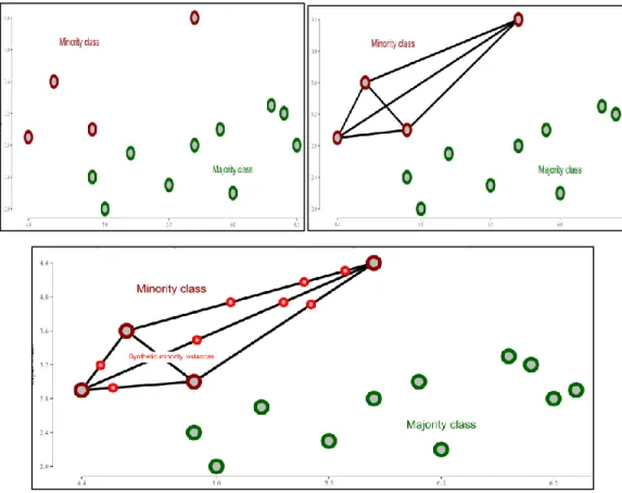
This method proposed by (Chawla, Bowyer, Hall & Kegelmeyer, 2002) is an efficient and widely used synthetic data generation oversampling technique in recent days. This method was proposed in place of oversampling with replacement method. Synthetic examples are generated by operating in ‘feature space’ instead of ‘data space. In this approach minority class is oversampled by introducing synthetic data points along the line segments joining k nearest neighbors. Neighbors from the k nearest neighbors are selected based on the oversampling ratio required.

Xnew = X + (X- X’) * rand (0,1)

where, X’ = k nearest neighbor, X = sample Synthetic samples are generated by multiplying the calculated difference between feature vector and its nearest neighbor with a random number between 0 and 1 and is added back to the feature vector (sample). This results in the selection of a random point along the line segment between two specific features. SMOTE mechanism can be explained as shown in Figure 2.1. The advantage of SMOTE is that it makes the decision regions larger and less specific with a drawback that it generates synthetic instances considering minority examples alone.

(22)

10

2.4.2 Modified Synthetic Minority Oversampling Technique

To improve the performance of SMOTE, a Modified Synthetic Minority Oversampling Technique (MSMOTE) was proposed by (Hu, Liang, Ma & He, 2009). Initially noise from the majority class is removed and the algorithm classifies minority instances into security samples, border samples and latent noise samples by calculating the distance between minority class samples and all the samples of the training dataset. If sample label in minority class is same as labels in k nearest neighbor then sample is security sample, sample is a noise in contrary and sample is borer if it doesn’t belong to any of the group. Furthermore, synthetic examples are generated for security samples by randomly choosing one of the k nearest neighbors and on application of this method, the results yielded was better than SMOTE.

2.5 Synthetic Data Generation Oversampling Method: Borderline Minority Samples

The examples on the borderline and the ones nearby are more likely to be misclassified by most of the classification algorithms which attempt to learn the borderline of each class during training process. Thus, the contribution of those examples farther away from the borderline are comparatively less than those which are present on and nearer to borderline. Pointing at these problems, (Han, Wang & Mao, 2005) proposed a technique named Borderline-SMOTE which included SMOTE-borderline1 and SMOTE-borderline 2

approaches which are slightly different form each other. 2.5.1 SMOTE- Borderline 1

In this approach, for every instance in the minority class, m nearest neighbor is calculated from the whole training dataset. The number of majority examples in the m nearest neighbors is denoted as m’. If all the m nearest neighbors are m’, then those examples are noise and is ignored from oversampling. If number of majority neighbors is greater than minority neighbors, then minority instances can be easily misclassified thus these are considered as instances at Danger. The minority instances can be considered safe if majority neighbors are less than minority neighbors. Likewise, the minority data points are categorized into noise, danger and safe before oversampling them.

(23)

11

Figure 2.1: SMOTE methodology in generating synthetic data points (Source: http://rikunert.com/SMOTE_explained)

The minority examples which are categorized into ‘Danger’ are the borderline data of minority class and are oversampled using SMOTE approach. Synthetic data is generated by multiplying the difference between each instance of the ‘Danger’ category with its s

nearest neighbors from minority class itself with a random number between 0 and 1. Synthetic examples are generated along the line between minority border line examples and their nearest neighbors of the same class, thus oversampling the borderline examples. 2.5.2 SMOTE- Borderline 2

In this technique, minority class examples are categorized into ‘safe’, ‘noise’ and ‘danger’ as categorized in previous approach. Synthetic data is generated by multiplying the difference between each instance of the ‘Danger’ category with its s nearest neighbors from minority class with a random number between 0 and 1. Likewise, Synthetic data is generated

(24)

12

by multiplying the difference between each instance of the ‘Danger’ category with its s

nearest neighbors from majority class but with a random number between 0 and 0.5 which will be closer to the minority class. Therefore, oversampling the borderline minority examples.

2.5.3 Safe-level-SMOTE

Safe-level-SMOTE was proposed by (Bunkhumpornpat, Sinapiromsaran & Lursinsap, 2009) to overcome the drawback of SMOTE and Borderline-SMOTE in generating synthetic instances in an unsuitable region where overlapping and noise exists degrading the performance of the classifiers. Here, each synthetic instance is generated in safe region by considering safe-level ratio of the instances. Initially, safe-level (sl) which is the number of minority instances in k-nearest neighbor is calculated followed by safe-level ratio. If the safe level is closed to 0 then it is nearly a noise and safe if it is closer to k.

Safe-level ratio = 𝑆𝑙𝑛

𝑆𝑙𝑝 where, Slp = the number of minority instances in k nearest neighbors for p in D

Sln = the number of minority instances in k nearest neighbors for n in D p is the minority instances in D dataset

n is the selected nearest neighbors of p.

Five decisions are made on the values obtained for safe level ratio while oversampling minority examples and is given in the following table (table 1).

SAFE LEVEL RATIO P, N INFERENCES

Safe level ratio = infinity p = 0 p and n are noises

Safe level ratio = infinity p != 0 n is noise

Safe level ratio = 1 p = n Synthetic instance will be generated along the line between p and n

(25)

13

Safe level ratio > 1 p > n synthetic instance is generated closer to p because p is safer than n.

Safe level ratio < 1 p < n synthetic instance is generated closer to n because n is safer than p

Table 2.1 : Safe-level SMOTE decision table

The experiment had a better performance when compared to SMOTE and Border-line SMOTE indicating that synthetic instances generated in safe regions can improve prediction performance of classifiers dealing with class imbalance problem.

2.6 Synthetic Data Generation Oversampling Method: Hard to Learn Minority Samples

(Garcia, 2008) proposed ADASYN which is used to adaptively generate minority data samples which are hard to learn by classifiers than those which are easy to learn. It is used to reduce the learning bias introduced by the imbalanced dataset and to adaptively shift the decision boundary to focus on those difficult to learn sample. Initially, the count of minority and majority samples are calculated followed by degree of class imbalance using,

d=minority class count / majority class count where, d € (1,0)

If the calculated degree of class imbalance is less than the threshold of maximum tolerated degree of imbalance, then the ADASYN approach is carried out which is as follows,

1. Calculate the number of synthetic data examples to be generated for the minority class using the following,

G = (majority class count – minority class count) * β where, β € (0,1)

(26)

14

β is the desired balance level to be maintained after the generation of synthetic points. If β = 1, fully balanced dataset will be created.

2. For each instance in the minority examples, K nearest neighbors is calculated based on Euclidean distance in n dimensional space and the following ratio is calculated.

ri =

𝛥𝑖 𝐾 where, i = 1 to instance in majority example count,

Δ is the number of examples in K nearest neighbors that belongs to majority class examples.

3. Normalize ri according to

rˆi = ri / ∑𝑚𝑖𝑛𝑜𝑟𝑖𝑡𝑦 𝑑𝑎𝑡𝑎 𝑖𝑛𝑠𝑡𝑎𝑛𝑐𝑒𝑠_𝑖=1 ri

where, rˆi is density distribution.

4. The number of synthetic data examples to be generated for each minority example is calculated using the following,

gi = ˆri * G

5. Synthetic data examples are generated by multiplying the difference between each randomly chosen minority data point with its k nearest neighbors of the same class with a random number between 0 and 1. The original data is updated with the addition of oversampled data.

The experiment outperformed SMOTE in terms of G-mean and accuracy.

2.7 SMOTE + SVM Classifiers

2.7.1 SVM On Imbalanced Data

SVM when applied on highly imbalanced datasets, its performance deteriorates significantly. While training an imbalanced dataset using SVM, class-boundary learned by SVM will be severely skewed resulting in high false negative rate. However, SVM can

(27)

15

perform well with moderately imbalanced data sets and it is unaffected by non-noisy negative instances far away from the boundary regardless of its count as it only considers the instances which are close to boundary line. (Akbani, Kwek & Japkowicz, 2004)

Causes of performance loss with Imbalanced dataset are:

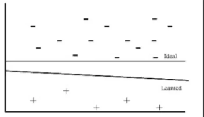
1. Positive Points Lie Further from the Ideal Boundary: In the case of imbalanced training data ratio wherein the negative instances outnumber positive instances, the minority data points might have situated farther away from the ideal boundary line as shown in the figure 2.2. Since, SVM considers the instances that is too close to the boundary, minority instances will be mis-classified as majority class instances.

Figure 2.2: Positive instances lie further away from the ideal boundary (horizontal line) than the negative instances. As a result, SVM learns a boundary (slanted line) that is too close to the positive support vectors (Akbani, Kwek & Japkowicz, 2004)

2. Weakness of Soft-margins: SVM is more focused in minimizing the mis-classification error by maximizing the margin. During this course of time, the penalty constant, C the trade-off between the empirical error and the margin which minimizes the error should be tuned properly. It is advisable to set the values of C as high with respect to minority class instances.

3. Imbalanced Support vector ratio: As the imbalanced ratio increases, ratio of support vectors will become more imbalanced. The neighborhood of a test instance close to the boundary will be more dominated by (majority class) negative support vectors and hence the decision function is more likely to mis-classify boundary point as majority class. To avoid this problem, increasing the weight of the minority class instances is advisable.

(28)

16

2.7.2 Synthetic Informative Minority Over-Sampling (SIMO) Algorithm Leveraging Support Vector Machine (SVM)

A novel method ‘Synthetic informative minority over-sampling (SIMO) algorithm leveraging support vector machine’ is proposed by (Piri, Delen & Liu, 2018). SIMO’s prime focus is on creating synthetic data points of informative minority data points alone. This can be achieved with the help of SVM, as data points that are close to the boundary of classes can be chosen as informative minority instances. The behavior of SVM on imbalanced datasets and use of these behavior in detecting informative instances during the application of SIMO is explained below.

The first and foremost step in performing SIMO is partitioning the dataset into train and validation dataset. To avoid bias, partition is carried out in such a way that constant imbalanced ratio is maintained in both train and validation dataset. Imbalanced gap which is the difference in count of minority and majority data instances is calculated for training dataset.

As briefed earlier, SVM misclassifies minority instances as majority instances when applied on highly imbalanced datasets. This might be because the minority data points lie further away from ideal boundary line due to which SVM tends to learn a boundary that is too close to the minority support vectors (Akbani, Kwek & Japkowicz, 2004). Thus, train data is trained using SVM and G-mean is computed. G-mean is the metrics which is usually calculated in the case of imbalanced data along accuracy. Higher the G-mean, better is the performance of the model.

Furthermore, Euclidean distance is calculated between the data point and the SVM decision boundary. As our major focus is informative minority data points and as mentioned earlier, data points close to the boundary of classes are important and informative and hence those data points with least Euclidean distance from decision boundary is identified as informative minority data instances. Using delta parameter, range of the data points with least Euclidean distance is selected as informative minority data points to oversample. Delta value is between 0 to 1 and for example if delta of value 0.2 is chosen, then top 20 percent of minority data points with least Euclidean distance value will be chosen for oversampling.

(29)

17

Synthetic data points are generated on the application of SMOTE oversampling technique on the informative minority data instances.

SIMO Algorithm

Given D, delta and p

Partition D into training and validation dataset.

1. Calculate Imbalanced gap, Imbalanced_gap = Majority_count – Minority_count 2. Develop initial SVM model on train dataset.

3. Compute Gmean ,

𝐺 − 𝑚𝑒𝑎𝑛 = √(𝑇𝑃𝑅 ∗ 𝑇𝑁𝑅)

4. Initialize, SVM = initial_SVM, G_Mean=G_Mean_initial, generated_data_count =0

While generated_data_count < Imbalanced_gap,

5. Calculate Euclidean distance of minority data points from Decision boundary.

6. Select top delta percent of minority data points close to boundary line based on calculated Euclidean distance. This will be regarded as informative minority data points. (delta = 0 to 1)

7. Oversample the chosen percent of minority data points using SMOTE approach. 8. Calculate the number of synthetic generated data points generated.

9. Update the initial training dataset with the resampled data. 10. Apply SVM and compute G_mean.

11. Update G_mean_initial with computed G_mean 12. End

13. Find the maximum G_mean and its index.

14. Select the oversampled training dataset with maximum G_mean.

15. Train the model of interest (Logistic regression and SVM linear) on final over-sampled training dataset

(30)

18

Notations:

D – Imbalanced Data set

delta–Top delta percent of minority data points that are close to decision boundary p – Oversampling degree for minority informative data points at each iteration

At this stage, the original imbalanced train data is updated with oversampled data. The number of synthetically generated data points and their indices will be recorded at each iteration. SVM will be applied on the updated training dataset. The decision boundary of this new SVM will be shifted toward the majority class data space closer to the ideal decision boundary as position of the SVM decision boundary only depends on the support vectors. The reason is that by generating synthetic minority examples, the imbalance ratio of the training dataset will be reduced along with an alleviated imbalance ratio of the support vectors. Performance of the SVM will be evaluated by computing the G mean and the Euclidean distance of the minority data points of an updated train dataset from the new SVM decision boundary is calculated, informative ones will be selected, and new synthetic minority data points will be generated. It is repeated until the number of synthetically generated examples reaches the imbalanced gap.

The performance of the model depends on the structure and complexity of the dataset. In each iteration, dataset will be updated with new synthetic generated minority examples. Though SVM improves on updated data set in each iteration, it isn’t guaranteed the same for all kinds of datasets. Hence the performance parameters are recorded for each iteration and the iteration with higher G mean value is identified as the best performing model and the training dataset associated with that iteration will be selected as final oversampled training dataset. This novel approach performed well regardless of learner algorithms used and generated comparably less synthetic data instance than other oversampling methods as the focus was on oversampling informative instance alone and hence reducing the computational cost.

2.7.3 Biased Support Vector Machine (SVM) And Weighed-SMOTE

Similarly, (Hartono, Sitompul, Tulus & Nababan, 2018) proposed Biased support vector machine and weighed-SMOTE in handling class imbalance problem. It is the

(31)

19

combination of Biased SVM and weighed-SMOTE techniques. (Gonzalez-Abril, Angulo, Nuñez & Leal, 2017) designed a preprocessing technique of modifying the bias of a standard SVM to improvise its performance on imbalanced dataset by fixing minimum value for recall, to maximize specificity on the training set and named the outcome as BSVM (Biased SVM). It is designed for scenarios where it is non-critical to increase true positive rate in trade-off with increase in false positive rate. BSVM achieved better performance in sensitivity and reduction in accuracy and hence (Prusty, Jayanthi & Velusamy, 2017) used weighed-SMOTE along to overcome the drawback.

The working of weighed-SMOTE is as shown in the figure 2.3. The Euclidean distance of each minority sample is collected with respect to the other minority data samples and then they are normalized using min-max normalization which is carried out to fit in the distance values in the range of 0 and 1. Remodeled Normalized Euclidean distance(RNED) represents that lesser Euclidean distance more the share it gets to generate synthetic samples out of total synthetic samples needs to be generated and hence RNED matrix can be given as the difference between normalized ED value of each minority data and sum of all the normalized ED values. Furthermore, weight matrix is calculated by dividing each minority data share fractionfrom the total sum of the shares in the RNED matrix, based on which Smote generation matrix is obtained.

(32)

20

In Biased support vector machine and weighed-SMOTE method, BSVM will classify classes into minority and majority support vectors(SV) sets and non-support vector(NSV) sets. Noises are removed from both minority and majority SV sets. NSV of Majority instances and SV of minority instances are processed using weighed-SMOTE approach. The NSV and SV of minority classes are combined to obtain new minority sample sets similarly the majority sample sets are obtained. The outcome of this experiment yielded satisfactory results in handling class imbalance with minority class in a high priority.

2.8 Cluster-Based Oversampling Methods

2.8.1 Cluster-SMOTE

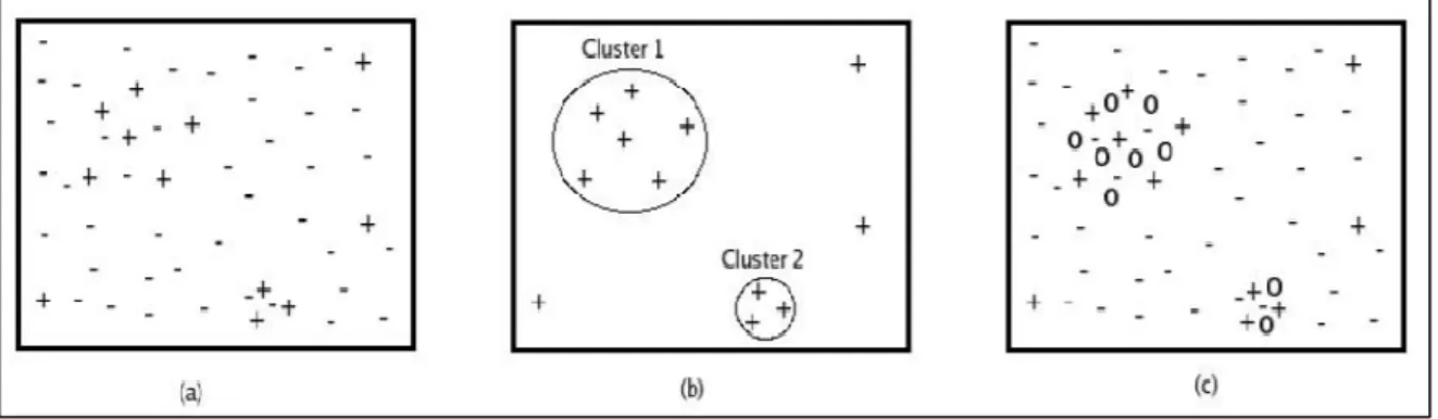
An addition to the existing methods are cluster-based methods where the dataset is reduced to clusters of similar class examples and those clustered instances are oversampled or under sampled. These approaches are focused on oversampling hard-to-learn instances (important information for the classifiers) which are usually available near decision boundary or belong to small concepts in the datasets which is referred as within-class imbalance. Cluster-SMOTE was proposed by (Cieslak, Chawla & Striegel, 2006), where k-means clustering is applied on the set of minority instances in the dataset and then SMOTE is applied on each cluster to oversample generating synthetic examples, and these are updated into the original dataset. These are advantageous in deriving the class regions and their borders for small group of minority examples which is as shown in the figure 2.4.

Figure 2.4: (a) features a sparse majority class, a minority class region, and many minority outliers. (b) Cluster-SMOTE detects two clusters of minority points and uses this information to generate new synthetic examples, as shown in (c) (Cieslak, Chawla & Striegel, 2006)

(33)

21

2.8.2 Adaptive semi-unsupervised weighted oversampling (A-SUWO)

A-SUWO a cluster-based oversampling method is proposed by (Nekooeimehr & Lai-Yuen, 2018). Minority instances are clustered using semi-supervised hierarchal clustering approach, the size of the sub cluster is determined based on the complexity of the sub-clusters in being mis-classified. It can be determined by a measurement parameter based on standardized average error rate which is obtained on cross validation. Synthetic examples are generated on assigning weights to the minority instances based on the average Euclidean distance to their NN-nearest majority neighbor. The advantage of this method is that it avoids generating overlapping synthetic data examples.

2.9 Oversampling + Under sampling approach

(Cateni, Colla & Vannucci, 2018) proposed a new sampling method named Similarity-based Under Sampling and Normal Distribution-based Oversampling (SUNDO) to balance the data without losing much of the significant data or adding up too much of unwanted synthetic patterns and it outperformed SMOTE approach. The method is the combination of both undersampling and oversampling techniques in achieving balanced data. Parameters k0 and k1, which represents minority and majority classes respectively are

to be set along with the number of N samples should be removed. N is calculated as follows, N = round (k1 * n0) – (k0 * n1)

3.0 Ensemble-based learning

Ensemble-based learning algorithms are playing predominant role in machine learning problems, especially while addressing class imbalance problem in many applications as it can improve the classification performance of any weak classifier. Ensemble learning is method of inclusion and combination of several classifiers to obtain new, better performing classifier. Ensemble based learning is the combination of ensemble based leaning and any of the imbalance learning approaches.

(Hao, Wang & Bryant, 2014) conducted an experiment with SMOTE coupled with GLMBoost to perform the classification of imbalanced datasets from PubChem BioAssay. The proposed experiment outperformed SMOTE in terms of performance metrices

(34)

22

Sensitivity and G-mean. Similarly, an empirical analysis to alleviate the class imbalance problem in heartbeat classification was carried out by (Rajesh & Dhuli, 2018), using data level sampling methods namely ROU, SMOTE+ RU and DBB and AdaBoost classifier and obtained significant performance measures. Henceforth, it can be concluded that, the application of data-level imbalance learning approach yielded better results with imbalanced dataset when combined with the learning algorithms irrespective of its complexity.

3.1 Summary of the Literature Review

The key focus of any sampling technique is to create a balance in the class distribution. Since, the dataset is small and highly imbalanced, the research is focused on the application of data-level imbalanced learning algorithms alone. Oversampling methods are advantageous over Under sampling as there will be no potential loss of information. Amongst the oversampling approaches, synthetic data generation is largely used, and its different approaches are reviewed in this section.

The advantage of SMOTE is, it broadens the decision region being less specific and generates artificial data points unlike Random Oversampling method, replicating the minority samples. Borderline-SMOTE majorly focus on those minority samples available near the borderline for oversampling. Since there is a suspicion of unsafe regions which would contain noisy data near the borderline, to ignore and oversample safe instances alone, Safe-level SMOTE was proposed. ADASYN is designed to detect and adaptively oversample those instances which are hard to learn by classifiers whereas SIMO using SVM oversamples informative data instance alone considering G-mean as the deciding performance metric which will be usually misclassified by the standard classifiers. Biased SVM with SMOTE is also designed for the same with an added tuning to the classifier SVM. Cluster oversampling focus on oversampling hard to learn instances which are found within-class imbalance whereas ensemble-based learners treats imbalance data by using ensemble learners along sampling approaches.

Although the methods are advantageous and yielded good performances there exist a shortcoming as well. Random oversampling might oversample noise minority data points

(35)

23

and is prone to problem of overfitting. The synthetic examples might be generated in overlapping and noise regions by Borderline-SMOTE. Problem of over generalization of synthetic data points that might lead to overlapping between classes can persist on the application of SMOTE. There can be an interpolation of a new sample between noisy data and one of its nearest neighbors in modified-SMOTE and ADASYN approaches. The generated minority instances in ADASYN will be slightly higher than majority instances which is in contrary with SIMO approach. This can have an influence on learner, training with high or insufficient samples. Also, the behavior of SVM on imbalanced dataset, role of SVM in improving the performance of imbalanced learning algorithms was discussed in this section.

In a nutshell, the extension and the adaption of SMOTE has produced improved results in terms of the model’s performance in treating minority class examples.

3.2 Gap in the research

Non-representative small dataset can hinder the performance of the classifiers as training size must be quite large and large test sample is essential to accurately evaluate classifier with low error rate. According to (Raudys & Jain, 1991), small sample size and small disjuncts are closely related topics. The lack of data, small disjuncts and noisy data are claimed to be interrelated challenges faced by researchers in imbalanced classification (Fernandez, Garcia, Herrera & Chawla, 2018).

‘Synthetic informative minority over-sampling (SIMO) algorithm leveraging support vector machine’ technique is implemented in this experiment. The advantages of this method over other methods are low computational training cost as the amount of synthetic data generated will be less, avoidance of overfitting, focus on informative minority instances alone and the use of efficient learner SVM (Piri, Delen & Liu, 2018). However, the algorithm’s performance is mainly dependent on distribution complexity and size of the datasets. Originally, SIMO has dealt with datasets of records ranging from 300 to 1500, yielding better performances when compared to other approaches. But the experiment is still not implemented on big data and very small dataset.

(36)

24

The values which should be considered for the parameters delta and p is specified in the paper with respect to the severity of class imbalance present in the data. It is advised to consider the values between 30 to 40 percent for delta and between 25 to 50 percent for p in high class imbalance scenarios. But these values being same for different size of the data is still in question. Performance of the classifiers can be influenced by size of the data as well and hence it is necessary to study, if performance of the classifiers on the implementation of this approach varies when applied on small datasets.

To study of the above-mentioned gaps following research question is proposed, “Can performance of the classifiers on small datasets, significantly improve on the application of ‘SIMO leveraging SVM’ over the application of baseline imbalanced learning algorithms?”

**SIMO: Synthetic Informative Minority Over-Sampling **SVM: Support Vector Machine

**Baseline imbalanced learning algorithms: SMOTE, SMOTE-Borderline1, SMOTE- Borderline2 and ADASYN.

(37)

25

CHAPTER 3 EXPERIMENT DESIGN AND METHODOLOGY

This chapter will give an account of the plan and methodology used to answer the research question by implementing the process involved in CRISP-DM reference model, an overview of data mining project lifecycle. The research starts from business understanding followed by data understanding, data preparation, modeling and evaluation covering five phases of the reference model (figure 3.1). Scikit-learn machine learning package available in python programming language is used to obtain results in support of the decision to reject or retain the hypothesis.

The objective of this research is to evaluate the performance of ‘Synthetic Informative Minority Over-Sampling leveraging SVM’ on the datasets of records less than 150 with imbalance ratio ranging from 20 percent to 40 percent, over other imbalanced learning algorithms; SMOTE, SMOTE-Borderline and ADASYN. The balanced dataset is trained using base classifiers SVM-Linear and Logistic regression and its performance metrices are obtained for comparison. The methodology and design used to achieve the above, is explained in each section of this chapter with respect to the CRISP-DM framework in detail.

(38)

26 3.1 Business Understanding

The research is mainly focused on the performance of Synthetic informative minority over-sampling (SIMO) algorithm leveraging support vector machine on very small imbalanced dataset of records less than 150, since the original paper has dealt with datasets of records more than 300. This novel algorithm have had performed comparatively better than others in the original paper, thus the aim of this paper is to measure its performance on very small datasets. Imbalanced learning algorithms like SMOTE, SMOTE- Borderline and ADASYN are chosen as baseline to compare and evaluate the hypothesis. The hypothesis to address the research question is as follows,

H0: “The G-mean and AUC of the models built on the oversampled datasets using

imbalanced learning algorithm SIMO is equal to the G-mean and AUC obtained from the models on application of baseline algorithms SMOTE, SMOTE-Borderline and ADASYN, with p-value < 0.05.”

** SIMO: Synthetic Informative Minority Over-Sampling **SMOTE - Synthetic Minority Over-Sampling Technique ** ADASYN - Adaptive Synthetic Sampling Approach

** AUC – Area Under Curve

3.2 Data Understanding

Datasets

Four datasets are used in this research paper out of which three are taken from UCI repository and one is collected in a time span of 5 years (2004 - 2009) from an European hospital. These are highly imbalanced data with records less than 150 and is chosen to validate performance improvement of the models when built on oversampled dataset by using a novel imbalanced learning algorithm, Synthetic informative minority over-sampling (SIMO) leveraging support vector machine over the models built by algorithms like SMOTE, SMOTE-Borderline and ADASYN which are readily available imbalanced learning packages in python. A brief description on the datasets is provided in the table below.

(39)

27 Dataset No. of records No. of features Imbalanced Ratio Minority class Majority class

Biomarker 93 51 60:40 ‘Yes’ ‘NO’

Hepatitis 154 20 80:20 ‘DIE’ ‘LIVE’

Echocardiogram 131 13 70:30 ‘ALIVE’ ‘DEAD’

Immunotherapy 90 8 80:20 ‘NO’ ‘YES’

Table 3.1: Dataset description

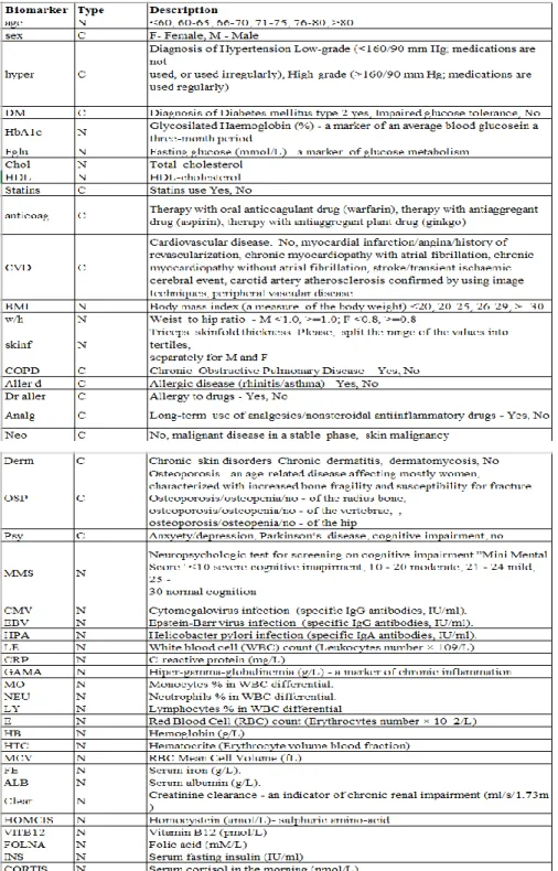
Dataset description:

1. Biomarker: This dataset contains 93 records with 51 features with a class imbalance ratio of 60:40. The Target variable is ‘Death’ which represents the mortality risk in elderly patients as ‘yes’ or ‘no’ in presence of specific biomarkers which are the independent variables or predictors. The variable description is as shown in table 3.2 below.

(40)

28

(41)

29

2. Hepatitis: The dataset contains 154 records with 20 features with a class imbalance ratio of 8:2. The Target variable is ‘Class’ which represents whether a patient with hepatitis is dead or alive. The variable description is as shown in table 3.3.

Attribute information:

VARIABLES TYPE DESCRIPTION

Class C DIE, LIVE

AGE N 10, 20, 30, 40, 50, 60, 70, 80

SEX C male, female

STEROID C no, yes

ANTIVIRALS C no, yes

FATIGUE C no, yes

MALAISE C no, yes

ANOREXIA C no, yes

LIVER BIG C no, yes

LIVER FIRM C no, yes

SPLEEN PALPABLE C no, yes

SPIDERS C no, yes

ASCITES C no, yes

VARICES C no, yes

BILIRUBIN N 0.39, 0.80, 1.20, 2.00, 3.00, 4.00

ALK PHOSPHATE N 33, 80, 120, 160, 200, 250

SGOT N 13, 100, 200, 300, 400, 500

ALBUMIN N 2.1, 3.0, 3.8, 4.5, 5.0, 6.0

PROTIME N 10, 20, 30, 40, 50, 60, 70, 80, 90

HISTOLOGY C no, yes

Table 3.3: Hepatitis dataset, C – Categorical variables, N – Numerical variables

(42)

30

3. Echocardiogram: This dataset contains 131 records with 13 attributes with a class imbalance ratio of 7:3. The target variable represents if the patient suffering from heart attack is dead (0) or is still alive (1). The description of independent variables is given in table 3.4.

Survival N the number of months, patient survived if they are dead and has survived, if patient is still alive.

still-alive C 0=dead,1=still alive

Age N age in years when heart attack occurred

pericardial-effusion

N Pericardial effusion is fluid around the heart. 0=no fluid, 1=fluid

fractional-shortening

N a measure of contracility around the heart lower numbers are increasingly abnormal

epss N E-point septal separation, another measure of contractility. Larger numbers are increasingly abnormal

lvdd N left ventricular end-diastolic dimension. This is a measure of the size of the heart at end-diastole. Large hearts tend to be sick hearts.

wall-motion-score N a measure of how the segments of the left ventricle are moving

wall-motion-index N equals wall-motion-score divided by number of segments seen. Usually 12-13 segments are seen in an echocardiogram. Use this variable INSTEAD of the wall motion score.

alive-at-1 C Boolean-valued. Derived from the first two attributes. 0 means patient was either dead after 1 year or had been followed for less than 1 year. 1 means patient was alive at 1 year.

(43)

31

4. Immunotherapy: It is a dataset of 90 records and 8 attributes with class imbalance ratio of 8:2. The target variable represents the response status of the patients on Immunotherapy treatment (wart treatment). This helps medical professionals in proceeding with the treatment if there is a positive response to the treatment from patient which is denoted as ‘Yes’ or to stop the treatment if the response is negative, represented as ‘No’. It saves time and money of both patients and the hospital.

Sex C “Man” = 1, “Women” = 2

Age N Age in years

Time N Time elapsed before treatment (month)

Number_of_Warts N 1 to 19

Type C Common, Plantar, Both

Area N Surface area of the warts (mm2) (6 – 900)

induration_diameter N 5 - 70

Result_of_Treatment C Yes, No

Table 3.5: Immunotherapy, C – Categorical variables, N – Numerical variables

An overview on the dataset can be derived from the following,

1. Descriptive statistics: This is carried out to obtain the details on central tendency (mean), median, mode, Inter-Quartile range, range, standard deviation and the skewness of the variables.

2. Missing value analysis: gives an account of missing value count and its percentage in the dataset with respect to each variable.

3. Exploratory data analysis: includes histograms to understand the distribution of numeric variables and to find out if there is any presence of outliers, frequency plots to analyze the relationship between categorical and numerical variables and correlation matrix to understand the relationship between numerical variables.

(44)

32

Based on the insights obtained from the above analysis, data preparation is carried out which is explained in the next phase in detail. The above analysis and visualization is carried out using available functions and packages in the python scikit-learn machine learning library.

Figure 3.2: Design Standardization and one-

hot encoding

Data Cleaning

Training dataset Test dataset

Imbalanced learning algorithms (SMOTE- Regular, Smote- Borderline,

ADASYN, SIMO)

Supervised learning algorithms (Logistic regression, Support Vector

Machine – Linear kernel)

(

Dataset

Performance

Evaluation metrices: Accuracy, specificity, Recall, Precision and G-Mean

DataUnderstanding

Standardization and one- hot encoding

(45)

33 3.3 Data Pre-Processing

In this phase, based on the understandings obtained from previous section, necessary data preparation methods are carried out which involves the following.

3.3.1 Data Imputation

Missing value analysis gives an overview on the missing value counts and its percentage with respect to each variable in the dataset. Data imputation is carried out on those whose values are missing. While imputation of numerical attributes, the histograms are also analyzed to detect if the data is prone to outliers as mean imputation will introduce a bias and is not advisable. On such cases median imputation will be carried out for continuous variables whereas mode imputation will be carried out for categorical variables. 3.3.2 Standardization: Z-Score

Numerical variables will have different impact on the predictive model in accordance with their ranges. Higher the range, higher the influence in prediction as predicters. Thus, the data should be scaled to fall under common range using Z-score standardization to improve the predictive accuracy. Standardization refers to shifting the distribution of each attribute to have a mean of zero and a standard deviation of one. It can be calculated as given below,

𝑧 − 𝑠𝑐𝑜𝑟𝑒 =𝑋−𝑋′

𝜎 Where, X = sample

X’ = mean of the sample

σ = standard deviation of the sample

The standard normal distribution of a dataset is as shown in the figure below (figure 3.3), which looks like a bell and thus called ‘Bell Curve’. It has a symmetry about the center which is referred as ‘mean’ whereas standard deviation is the measure of quantifying the amount of dispersion of the data. Low standard deviation values usually will be closed to the mean whereas high standard deviation values denote how spread out the values are.