Compassionately Conservative Normalized Cuts for Image Segmentation

Rochester Institute of Technology

Rochester Institute of Technology

RIT Scholar Works

RIT Scholar Works

Theses

3-7-2017

Compassionately Conservative Normalized Cuts for Image

Compassionately Conservative Normalized Cuts for Image

Segmentation

Segmentation

Tyler L. Hayes

[email protected]

Follow this and additional works at: https://scholarworks.rit.edu/theses

Recommended Citation

Recommended Citation

Hayes, Tyler L., "Compassionately Conservative Normalized Cuts for Image Segmentation" (2017). Thesis. Rochester Institute of Technology. Accessed from

This Thesis is brought to you for free and open access by RIT Scholar Works. It has been accepted for inclusion in Theses by an authorized administrator of RIT Scholar Works. For more information, please contact

Compassionately Conservative

Normalized Cuts for Image

Segmentation

by

T

yler

L. H

ayes

A Thesis Submitted in Partial Fulfillment of the Requirements

for the Degree of Master of Science in Applied and Computational Mathematics

School of Mathematical Sciences, College of Science

Rochester Institute of Technology

Rochester, NY

Committee Approval:

Nathan Cahill, D.Phil.

School of Mathematical Sciences

Thesis Advisor

Date

Elizabeth Cherry, Ph.D.

School of Mathematical Sciences

Committee Member

Date

John Hamilton Jr., Ph.D.

School of Mathematical Sciences

Committee Member

Date

Sogol Jahanbekam, Ph.D.

School of Mathematical Sciences

Committee Member

Date

Christopher Kanan, Ph.D.

Center for Imaging Science

Committee Member

Date

Matthew Hoffman, Ph.D.

School of Mathematical Sciences

Director of Graduate Programs

Abstract

Image segmentation is a process used in computer vision to partition an image into regions with similar characteristics. One category of image segmentation algorithms is graph-based, where pixels in an image are represented by vertices in a graph and the similarity between pixels is represented by weighted edges. A segmentation of the image can be found by cutting edges between dissimilar groups of pixels in the graph, leaving different clusters or partitions of the data.

A popular graph-based method for segmenting images is the Normalized Cuts (NCuts) algorithm, which quantifies the cost for graph partitioning in a way that biases clusters or segments that are balanced towards having lower values than unbalanced partitionings. This bias is so strong, however, that the NCuts algorithm avoids any singleton partitions, even when vertices are weakly connected to the rest of the graph. For this reason, we propose the Compassionately Conservative Normalized Cut (CCNCut) objective function, which strikes a better compromise between the desire to avoid too many singleton partitions and the notion that all partitions should be balanced.

We demonstrate how CCNCut minimization can be relaxed into the problem of computing Piecewise Flat Embeddings (PFE) and provide an overview of, as well as two efficiency improvements to, the Splitting Orthogonality Constraint (SOC) algorithm previously used to approximate PFE. We then present a new algorithm for computing PFE based on iteratively minimizing a sequence of reweighted Rayleigh quotients (IRRQ) and run a series of experiments to compare CCNCut-based image segmentation via SOC and IRRQ to NCut-based image segmentation on the BSDS500 dataset. Our results indicate that CCNCut-based image segmentation yields more accurate results with respect to ground truth than NCut-based segmentation, and IRRQ is less sensitive to initialization than SOC.

Acknowledgments

First and foremost, I would like to express my sincere gratitude to my advisor, Dr. Nathan Cahill, for his continuous support of my Master’s study and research, his patience, wisdom, motivation, and his utmost passion for research. He has helped not only guide me, but push me in all aspects to grow as a researcher, and for this I am extremely grateful.

Moreover, I would like to thank my committee members, Dr. Elizabeth Cherry, Dr. John Hamilton Jr., Dr. Sogol Jahanbekam, and Dr. Christopher Kanan for their immense knowledge, time, helpful comments, and thought-provoking questions. Additionally, I would like to thank Renee Meinhold for her theoretical and experimental contributions detailed in this thesis. I would also like to thank the RIT School of Mathematical Sciences for allowing me to pursue two degrees within their department and for providing me with the invaluable resources to grow as a mathematician.

I must also express my profound gratitude to my family and friends for their unfailing love and support. In particular, I must thank my mom for continually believing in me and encouraging me to chase my passion. Finally, a special thanks to James Arnold whose unconditional love, support, and patience have provided me with constant motivation and encouragement throughout my college career.

Contents

1 Introduction 1

2 Prior Work and Research Aims 3

2.1 Introduction to Image Segmentation Methods . . . 3

2.2 Prior Graph-Based Work . . . 4

2.3 Research Aims . . . 6

3 Compassionately Conservative Normalized Cuts (CCNCuts) 8 3.1 Definition of the CCNCut . . . 8

3.2 Relaxation of the CCNCut . . . 10

4 Two-Stage Numerical Approach to Solving the Piecewise Flat Embedding (PFE) Prob-lem 12 4.1 Overview of the Two-Stage Numerical Approach . . . 12

4.2 Efficient Computation of the PFE Problem . . . 14

4.3 Two-Stage Approach for Segmentation . . . 16

4.4 Performance Comparison Between Algorithms Against Ground-Truth . . . 18

5 Piecewise Flat Embeddings (PFE) with Iteratively Reweighted Rayleigh Quotients (IRRQ) 21 5.1 Iteratively Reweighted Rayleigh Quotients Minimization Algorithm . . . 21

5.2 Solving Step (a) of the IRRQ Algorithm . . . 22

5.3 Choosingκ for Rapid Convergence . . . 24

6 Segmentation Experiments and Results 25 6.1 Segmentation Experiments . . . 25

6.2 State-of-the-Art on BSDS500 . . . 26

6.3 Results . . . 26

6.4 Comparison of Algorithms for CCNCut Minimization . . . 30

7 Conclusions and Future Work 37 7.1 Conclusions . . . 37

7.2 Future Work . . . 38

8 Appendix 39 8.1 Proof of Lemma 5.1 . . . 39

List of Figures

1 An example of NCuts yielding a better partition of the data than the Minimum Cut [20]. . . 6 2 (a) A graph we wish to partition into three subgraphs; all edges have unit weight

except for the two edges with weightα ∈ (0, 1). Partitioning solutions differ

based on whetherαfalls above or below a critical valueα∗. (b) Minimizing the

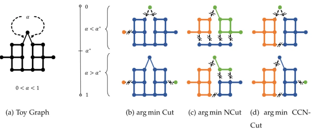
3-way cut (Cut) yields configurations in which two single vertices are removed. (c) Minimizing the 3-way Normalized Cut (NCut) avoids singleton subgraphs, but forces cuts between strongly-connected vertices in order to yield “balanced” solutions. (d) Minimizing the 3-wayCompassionately Conservative Normalized Cut (CCNCut) enables singleton partitions where vertices are weakly connected to the rest of the graph, but retains balance between the remaining partitions. . . . 9 3 The two-stage approach using the SOC algorithm [13] paired with the Split

Bregman algorithm [11] to solve the`1-minimization problem in (3.9) subject to an orthogonality constraint. The PFE is a result of the combination of stages 1 and 2. . . 14 4 The gPb signal and resulting affinity matrix from an image in the BSDS500

dataset at one-quarter the original resolution. The resized image resolution is 121×81 pixels in this example. . . 17 5 Computation times for the efficient implementation of PFE based on the intensity

and gPb graph constructions. . . 20 6 BSDS500 test images and segmentation results with intensity graph construction:

(a) original, (b) NCut, (c) CCNCut by SOC initialized with Laplacian Eigenmaps, (d) CCNCut by IRRQ, (e) CCNCut by SOC Initialized with Gaussian mixture model, (f) CCNCut by IRRQ initialized with Gaussian mixture model. . . 32 7 BSDS500 test images and segmentation results with gPb graph construction: (a)

original, (b) NCut, (c) CCNCut by SOC initialized with Laplacian Eigenmaps, (d) CCNCut by IRRQ, (e) CCNCut by SOC Initialized with Gaussian mixture model, (f) CCNCut by IRRQ initialized with Gaussian mixture model. . . 33 8 BSDS500 test image with CCNCut-based segmentation using the IRRQ algorithm

with the gPb graph construction for various values ofk. . . 34 9 Computation times for CCNCut-based segmentation of BSDS images for various

numbers of segments based on gPb graph construction. Algorithms are all initialized with LE. . . 34

10 Covering, PRI, and VI between segmentations generated from GMM and LE initializations of each CCNCut minimization method based on (a) intensity graph construction and (b) gPb graph construction. . . 35 11 Minimization of the cost function for a particular image as a function of number

List of Tables

1 Comparison of Yu et al. implementation of PFE (Yu-PFE) and our efficient PFE method (Ours) on the BSDS5000 dataset using the intensity-based affinity construction. All results were averaged across images and the best results for each performance measure have been highlighted in bold. . . 19 2 Comparison of Yu et al. implementation of PFE (Yu-PFE) and our efficient PFE

method (Ours) on the BSDS5000 dataset using the gPb-based affinity construc-tion [1]. All results were averaged across images and the best results for each performance measure have been highlighted in bold. . . 19 3 Comparison of various segmentation methods on the BSDS500 dataset. ‘MCG’

denotes results produced by the Multiscale Combinatorial Grouping method [2]. ‘PFE + mPb’ and ‘PFE + MCG’ denote results produced by the Piecewise Flat Embedding technique using global contour information [27]. ‘SAA’ denotes results produced by the Scale-Aware Alignment technique [7]. ‘FCNN’ and ‘FCNN + HED’ denote results produced by the FCNN strategy both without and with the holistically-nested edge detection scheme respectively [24]. Best results for each performance measure highlighted in bold. . . 27 4 Comparison of various segmentation methods on BSDS500 test set using intensity

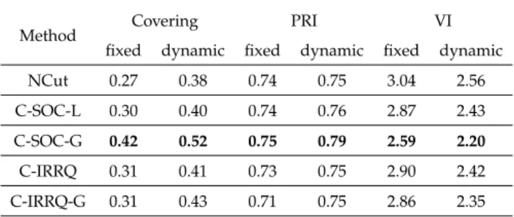
graph construction, averaged across images. Best results for each performance measure highlighted in bold. . . 28 5 Comparison of various segmentation methods on BSDS500 test set using gPb

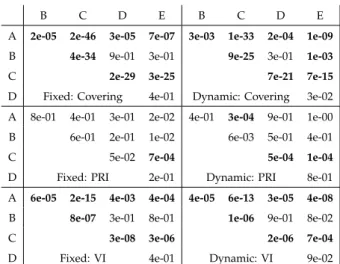
graph construction, averaged across images. Best results for each performance measure highlighted in bold. . . 28 6 p-values of two-sided Wilcoxon rank sum tests for the intensity graph

construc-tion at which we would reject the null hypothesis that performance measures computed from methodsiandjhave the same medians. Methods are: (A) NCut, (B) C-SOC-L, (C) C-SOC-G, (D) C-IRRQ, (E) C-IRRQ-G.p-values less than 0.05 are highlighted in bold. . . 29 7 p-values of two-sided Wilcoxon rank sum tests for the gPb graph construction at

which we would reject the null hypothesis that performance measures computed from methods i and j have the same medians. Methods are: (A) NCut, (B) C-SOC-L, (C) C-SOC-G, (D) C-IRRQ, (E) C-IRRQ-G.p-values less than 0.05 are highlighted in bold. . . 29

1

Introduction

In computer vision, image segmentation is the process by which a machine automatically segments an image into regions with similar characteristics. These segmented images often have diverse applications ranging from helping doctors identify tumors to serving as a pre-processing step in most modern computer vision and machine learning algorithms. As a pre-processing step, image segmentation is useful in providing initial estimates for tasks such as detection, recognition, and tracking of objects in both images and videos. While automating the task of image segmentation is known to be a challenging problem, automation can alleviate the need for human analysts with the added benefit of improved segmentation accuracy.

Image segmentation algorithms fall into a wide variety of categories, but one of the most popular is graph-based segmentation algorithms. A graph-based image segmentation algorithm is one that treats an image as a graph with vertices representing pixels and weighted edges representing the similarity between pixels. The algorithm then cuts edges between dissimilar groups of pixels, leaving different segments or partitions of the original image. One such algorithm is the Normalized Cuts (NCuts) algorithm [19, 20], which minimizes a normalized sum of weighted edges removed between groups of pixels in a graph. By normalizing the cut cost by the total degrees of each partition, the user eliminates trivial segmentations of the data, where a partition consists of a single pixel.

We argue that in some cases the NCuts algorithm goes too far in keeping partitionsbalanced, which often yields segments that look unnatural. In this thesis, we present a new cut cost which strikes a compromise between the desire to avoid too many singleton partitions and the notion thatall partitions should be balanced. This new cut cost, coinedCompassionately Conservative Normalized Cuts(CCNcuts), normalizes the original cut cost by thesquare rootof the total degrees of each partition. The CCNCut is more conservative in its normalization scheme than the original NCuts algorithm, which normalized by the total degrees of each partition. Computing solutions that minimize these various cuts is NP-hard. For NCuts, one way to efficiently approximate the solution is to relax the discrete minimization problem into a continuous one; the relaxed problem can then be transformed into a generalized eigenvalue problem. The relaxed problem is equivalent to the Laplacian Eigenmaps (LE) problem [4], which is a well-known technique for computing representations of data on manifolds. We will show in Chapter 3 that CCNCuts can be relaxed in a similar manner, yielding a continuous relaxation that coincides with the Piecewise Flat Embedding (PFE) problem [27]. The PFE problem is a weighted`₁-minimization subject to a quadratic (orthogonality) constraint.

To compute an approximation to the PFE problem, Yu et al. [27] introduced an iterative scheme based on the Splitting Orthogonality Constraint (SOC) algorithm [13]. While this algorithm demonstrated promising results on the BSDS500 dataset [1], we found that it was not computationally feasible for large images. However, we were able to propose two improvements that are described in Chapter 4 [16]*. The first improvement involves reformulating the original PFE problem to allow multiple linear algebra computations to be performed in parallel. The second improvement utilizes the preconditioned conjugate gradient iterative linear solver to quickly solve a succession of linear least-squares problems.

While the technique for solving PFE based on the SOC algorithm yielded promising results, there are some limitations to this approach. First, the algorithm relies on nested iterations of two algorithms that each have their own set of parameters that must be tuned. Second, due to the nested iterations approach, the algorithm does not strictly enforce the orthogonality constraint in the second loop, which means that the SOC algorithm is not actually approximating a solution to the exact PFE problem. Finally, the SOC algorithm requires an initial estimate of the embedding and can be highly sensitive to initialization.

Due to these limitations, in Chapter 5, we propose an alternative approach for solving the PFE problem inspired by the Iteratively Reweighted Least Squares (IRLS) algorithms commonly used to solve`1-minimization problems [9]. IRLS algorithms perform`1-minimization by iteratively solving a succession of weighted least-sqaures (`2-minimization) problems, with the weights updated at each iteration to reduce the impact of large residual errors. The advantage of IRLS algorithms is that they do not require an initial estimate of the embedding, although they can certainly be provided with one, and in specific cases [9], they have provable convergence guarantees. We show that the solution to the PFE problem can be approximated by iteratively solving a succession of weighted Rayleigh Quotient minimization problems, and thus we term this new algorithmIteratively Reweighted Rayleigh Quotient(IRRQ) minimization.

In Chapter 6, we demonstrate results of minimizing CCNCuts by solving the relaxed (PFE) problem using the IRRQ algorithm on the BSDS500 dataset [1] in a series of experiments. We then provide a detailed comparison of the original SOC algorithm to our proposed IRRQ algorithm. Finally, in Chapter 7 we provide conclusions as well as a list of open questions pertaining to the PFE problem.

*_{The proposed computational improvements to the SOC algorithm for computing PFE that are described in Chapter} 4 of this thesis were done in collaboration with Renee Meinhold.

2

Prior Work and Research Aims

2.1

Introduction to Image Segmentation Methods

Although the main objective of image segmentation is to group pixels into regions with similar characteristics, there are a wide variety of methods to choose from when performing segmen-tation. At the highest level, these methods could be considered threshold-based, edge-based, region-based, energy-based, or graph-based, with some algorithms combining several of these techniques.

Threshold-based methods are most commonly used for binary or gray-scale image segmentation. In these methods, a threshold is chosen based on some criteria, and pixels are assigned discrete labels based on whether they fall above or below this value. Often, a histogram of pixel values is generated, and large ‘peaks’ in the histogram counts distinguish the threshold values that should be chosen. One of the most common thresholding algorithms for segmentation isk -means clustering where initial cluster centers can be chosen based on thresholding a histogram of intensity values.

Edge-based methods form segmentation boundaries based on local or global edge and contour information in an image. Three of the most common contour or edge-based segmentation methods are the watershed algorithm [22], snakes [12], and level set methods such as fast marching methods [18]. These methods are useful in locating boundaries on images in an iterative fashion and, as such, are often coined active contouralgorithms [21]. In Chapter 4, we introduce the global probability of boundary (gPb) method [1] which yields a probability distribution of boundaries over an image.

Region merging techniques for segmentation fall into two main categories: region splitting techniques and region merging techniques. Region splitting, or divisive clustering, techniques treat the initial image as a single cluster, and use either thresholding or cost function optimiza-tion to partioptimiza-tion an image into smaller clusters. Region merging, or agglomerative clustering, techniques initially treat each pixel as a single cluster, and iteratively merge pixels with similar characteristics into larger clusters.

The similarity between each of these methods is in their ability to produce segmentations with small intra-pixel variability among clusters. If we add the restriction that pixels must be grouped together when they have small relative distances, then we have added a constraint to the segmentation problem. This constraint allows the segmentation problem to be reformulated as an energy function optimization problem, which can be formed using either a variational

formulation or a Markov random field (MRF). In the next section, we introduce the notion of graph-based segmentation, where an image is represented as a graph, and a partitioning of the data is found by optimizing a cost function involving the relationships between vertices in the graph.

2.2

Prior Graph-Based Work

Graph-based image segmentation algorithms have been of interest to the computer vision community due to their ability to model the relationship between pixels within a given neighborhood of an image. In these algorithms, the original image is modeled as an undirected, weighted graph with pixels represented by nodes and the similarity between pixels represented by weighted edges.

Consider an undirected weighted graphG = (V,E)that we wish to partition into two disjoint subgraphs,GA= (A,EA)andGB= (B,EB)whereASB=V. This partitioning can be achieved

by removing orcutting the edges connecting Aand B. The associated cost of this partition ofG is known as the cut cost and is defined as the total weight of the edges that have been removed:

Cut(A,B) =

∑

vi∈A,vj∈B

Wi,j , (2.1)

whereV={v1,v2, ...,vn}is the vertex set andWis the weighted adjacency matrix of the graph G.

One method to find an optimal partitioning ofGwould be to minimize (2.1) to find the minimum cut. The issue with the minimum cut, however, is that oftentimes the optimal partitioning leaves one subgraph with a single vertex [23]. A demonstration of this can be observed in Figure (1), in which the normalized cut, a cut that will be introduced in (2.3), yields a more desirable partioning of the data than the minimum cut due to its ability to maintain balanced partitions. To determine a more balanced partition, other cut costs have been proposed, including the Ratio Cut (RCut) [6]

RCut(A,B) = Cut(A,B)

(|A| · |B|) , (2.2)

and the Normalized Cut [19, 20]

NCut(A,B) = Cut(A,B) Assoc(A,V)+ Cut(A,B) Assoc(B,V) , (2.3) where Assoc(S,V) =

∑

vi∈S,vj∈V Wi,j (2.4)

In [20], it is shown that minimizing (2.3) is equivalent to solving the discrete minimization problem: min y yT(D−W)y yT_Dy subject to yi∈ {1,−b},i=1, 2, ...,n, yTD1=0 , (2.5)

whereDis the diagonal weighted degree matrix of the graphGdefined componentwise by di = Di,i = ∑jWi,j,b = (∑xi>0di)/(∑xi<0di), andy = (1+x)/2−b(1−x)/2, wherex is an

n-dimensional indicator vector wherexi = 1 if vertex vi is inAand xi = −1 otherwise. It

is then shown that if (2.5) is relaxed such that all components ofy∈ R, then the solution is equivalent to the generalized eigenvector corresponding to the smallest nontrivial eigenvalue of

(D−W)y=λDy . (2.6)

The components of the resulting eigenvector can then be clustered using an algorithm, such as k-means, and then assigned a discrete label.

Note that this formulation of the relaxed minimization problem is mathematically equivalent to that of Laplacian Eigenmaps (LE) [4], where it is assumed that the data being analyzed lie on a manifold that is embedded in a high-dimensional space. LE attempts to reduce the dimensionality of the data by seeking a mapping such that data points with similar attributes in the original space retain small distances in the new feature space. If the new feature space has dimension one, then LE can be expressed as the following constrained minimization problem: min y

∑

i,j Wi,jkyi−yjk22 subject to yTDy=I yTD1=0 . (2.7)

The orthogonality constraintyTDy=Iensures that the final data embedding is non-trivial, and the balance constraintyTD1=0is necessary to avoid the trivial eigenvalue and to ensure that partitions in the final data embedding arebalanced. A difficulty with using LE, however, is that while pixels with small local distances in the original feature space retain this relationship in the final embedding, pixels in the final data embedding may still be far enough apart that assignment of discrete labels is often ambiguous.

An ideal embedding of data in a new feature space would distribute pixels of the same region tightly around a single point, while pushing pixels of different classes apart to eliminate the ambiguity of cluster boundaries in the new feature space. The Piecewise Flat Embedding (PFE) [27] was proposed to achieve this goal and does so by modifying the LE objective function

Figure 1: An example of NCuts yielding a better partition of the data than the Minimum Cut [20].

to use an`<sub>1</sub>-norm. The use of an`₁-norm in minimization promotes sparse solutions to the segmentation problem, which makes the assignment of discrete labels to pixels a trivial process [27]. The PFE problem can be expressed as the constrained minimization problem:

min y

∑

i,j Wi,jkyi−yjk1 subject to yTDy=I . (2.8)

Incorporating the`₁-norm promotes sparse solutions such that pixels in the new feature space that belong to the same class have distances close to zero, while pixels belonging to different classes have much larger distances. This makes segmentation in the new feature space a straightforward process.

In addition to their introduction of the PFE problem [27], Yu et al. also introduced a two-stage numerical approach to solving (2.8), which we will further outline in Chapter 4. Although this two-stage approach yielded promising results on a publicly available dataset, the method does not scale well to large images, requires an initial estimate of the data embedding, and, due to its two-stage nature, has two different sets of parameters that must be tuned at each stage.

2.3

Research Aims

The main goals of this thesis are (1) introducing a new cut cost that, when relaxed, yields the PFE problem, (2) proposing computational improvements made to the two-stage numerical approach introduced in [27], (3) introducing a new algorithm for computing the PFE, and (4) illustrating how image segmentation performed with our new cut cost outperforms the SOC algorithm proposed in [27].

cut [23] and the normalized cut [19, 20]. While our new cut cost allows for singleton partitions as in [23], the new cut cost still maintains a notion of normalization, albeit to a lesser extent than the original normalized cut, that significantly reduces the number of singleton partitions in the final pixel labeling.

In Chapter 4, we demonstrate two computational improvements made to the algorithm in-troduced in [27] to allow the method to scale to larger images. We use these computational improvements to generate our own MATLAB implementation of the algorithm to reproduce the results generated in [27] and to utilize in our own experiments.

In Chapter 5, we introduce our new algorithm for solving the PFE problem. The inspiration for our algorithm came from the Iteratively Reweighted Least Squares (IRLS) algorithms typ-ically used for`1-minimization. The advantages of the IRLS algorithms are that they do not require an initial estimate of the data embedding and, in special cases [9], have provable linear convergence guarantees. Our algorithm seeks to overcome the shortcomings of the two-stage numerical approach presented in [27] by only requiring the tuning of a single hyperparameter and ensuring convergence to the global minimum independent of embedding initialization. In Chapter 6, we illustrate the use of CCNCuts for image segmentation on a publicly available database of images. We then compare the results from the SOC algorithm to our proposed algorithm and discuss the benefits and limitations of each algorithm.

3

Compassionately Conservative Normalized Cuts (CCNCuts)

In this Chapter, we introduce the Compassionately Conservative Normalized Cut (CCNCut), which provides an alternative normalization to NCut. When minimized, CCNCut yields graph partitions in such a way that few singleton partitions are permitted, but the notion ofbalanced partitions still exists. Consider the example presented in Figure (2), where we wish to partition the toy graph into three subgraphs. This toy graph (2a) contains 15 vertices and 19 edges; all but two of the edges have unit weight, and the two indicated edges have weightα∈(0, 1). For

each cost function, the three-way partitioning of minimum cost depends on whetherαfalls

above or below some critical valueα∗. As expected, when the three-way Cut cost is minimized,

the resulting partitions are heavily unbalanced, as shown in (2b).

While the three-way NCut cost (thek-way NCut cost is defined in [25]) yields more balanced partitions shown in (2c), the Cut costs of these partitionings are relatively high and these partitions do not necessarily look “natural” from a gestalt sense. We argue that the partitions demonstrated in (2d) have a more “natural” look than those in (2b), striking a compromise between the partitionings resulting from the Minimum Cut (2b) and the Normalized Cut (2c). The partition depicted in (2d) is our proposed Compassionately Conservative Normalized Cut, which differs from NCuts in its normalization by thesquare rootof the total degrees of each partition. This normalization is more conservative than the original NCuts formulation, allowing us the flexibility to obtain singleton partitions, while also maintaining a notion of balanced partitions. For natural imagery, this flexibility allows more realistic partitions of the data to be obtained.

3.1

Definition of the CCNCut

Consider an undirected weighted graphG = (V,E)that we we wish to partition intokdisjoint subgraphs,Gi= (Vi,Ei),i=1, 2, . . . ,k, whereSki=1Vi=V. G can be partitioned by removing

edges connecting each of the subgraphs to every other subgraph. To find an optimal partitioning of G, we must define and optimize a partitioning cost. A standard partitioning cost that is analogous to the minimum cut cost is themultiway cut cost, defined as the total weight of the edges that have been removed:

Cut(V1, . . . ,Vk) = 12

k

∑

`=1

0 1

(a) Toy Graph

∗ ∗ ∗

1 0

(b) arg min Cut (c) arg min NCut (d) arg min

CCN-Cut

Figure 2: (a) A graph we wish to partition into three subgraphs; all edges have unit weight except for the two edges with weightα∈(0, 1). Partitioning solutions differ based on whetherα

falls above or below a critical valueα∗. (b) Minimizing the 3-way cut (Cut) yields configurations

in which two single vertices are removed. (c) Minimizing the 3-way Normalized Cut (NCut) avoids singleton subgraphs, but forces cuts between strongly-connected vertices in order to yield “balanced” solutions. (d) Minimizing the 3-wayCompassionately Conservative Normalized Cut(CCNCut) enables singleton partitions where vertices are weakly connected to the rest of the graph, but retains balance between the remaining partitions.

where the pairwise cut cost is defined by:

Cut(A,B) =

∑

vi∈A,vj∈B

wi,j , (3.2)

the vertex setV={v1,v2,· · ·,vn}, andWis the weighted adjacency matrix (oraffinitymatrix)

ofGcontaining only positive weights. Since the graphG is undirected,Wwill be symmetric. Minimizing this Cut cost is undesirable, however, as it can yield partitionings in which one or more of the subgraphs contain a single vertex [23]. More balanced partitions emerge if the pairwise cut costs are normalized by the total degrees (volumes) of the subgraphs. Yu and Shi [25] define a multiway generalization of the NCut cost [19, 20] by:

NCut(V1, . . . ,Vk) = 12 k

∑

`=1 Cut(V`,V\V`) Vol(V`) , (3.3)

where Vol(V`) =∑vj∈V`dj, anddj=∑mwj,mis the degree of vertexvj.

Instead of normalizing the pairwise cut costs by the volumes of each subgraph, we propose normalizing by the square roots of the volumes:

CCNCut(V1, . . . ,Vk) = 12 k

∑

`=1 Cut(V`,V\V`) p Vol(V`) . (3.4)

In simple terms, minimizing the CCNCut cost (3.4) should still yield partitions that are more balanced than when minimizing (3.1), while better preserving strongly-connected subgraphs than when minimizing (3.3).

By defining ann×kindicator matrixXsuch thatXi,j =1 ifvi∈VjandXi,j=0 otherwise, it

is straightforward to see how (3.3)–(3.4) can be reformulated. Ifxi is theithcolumn ofX, then

Vol(Vi)can be written in terms of the degree matrixD=diag(d)asxTi Dxi, and the pairwise

cut cost betweenViandV\Vican be written as Cut(Vi,V\Vi) =xTiW(1−xi) =xiTd−xTi Wxi =

xT

iDxi−xTiWxi = xTiLxi, whereL=D−Wis the graph Laplacian matrix. This allows us to

express (3.3)–(3.4) as: NCut(V1, . . . ,Vk) = 1₂ k

∑

`=1 xT<sub>`</sub>(D−W)x` xT `Dx` , (3.5) CCNCut(V1, . . . ,Vk) = 12 k

∑

`=1 xT<sub>`</sub>(D−W)x` q xT<sub>`</sub>Dx` . (3.6)

Minimizing (3.3)–(3.4) is equivalent to minimizing (3.5)–(3.6) subject to the constraint thatXTX

is positive diagonal, which ensures that none of theVi’s will collapse to the empty set.

3.2

Relaxation of the CCNCut

Minimizing (3.6) is NP-hard, as is minimizing (3.5). However, relaxing (3.6) yields a problem whose solution can be efficiently approximated. To relax the CCNCut, we use an argument similar to Yu and Shi [25] in their relaxation of the NCut. From [25], we see that if Y = X XTDX−1/2

, then YTDY = I and (3.5) is equivalent to tr YTLY

. Hence, the solution to minimizing a relaxed version of (3.5) isY˜ =UQ, whereUis then×kmatrix whose columns are the orthonormal eigenvectorsu2, . . .,uk+1corresponding to the smallest nontrivial eigenvalues of D−1/2LD−1/2, and Q is an arbitrary k×k orthogonal matrix. The optimal solutionX˜ to (3.5) can then be approximated byk-means clustering [17], nonmaximal suppression [25] or Procrustean rounding [28] onY˜.

Now define ˆyi to be theithrow ofY. We then have that the minimization of the relaxed version

of (3.5) is equivalent to solving the constrained minimization problem: min Y∈Rn×k J2(Y):= n

∑

i=1 n

∑

j=1 wi,j ˆy_i−ˆy_j 2 2 (3.7) subject to: YTDY=I , YTD1=0 ,

which is identical to the Laplacian Eigenmaps (LE) problem [4] for computing embeddings of data that are assumed to lie on a manifold. Recall that thebalance constraintYTD1= 0is

necessary to avoid eigenvectors ofD−1/2LD−1/2corresponding to the trivial eigenvalue. Turning our attention now to (3.6), if we defineα_` =

∑idix2_i,` −1/2

for `=1, . . . ,k, and we note that XTDX−1/2

=diag(α), we can write:

CCNCut(V1, . . . ,Vk) = k

∑

`=1 ∑i,jwi,j xi,`−xj,` 2 ∑idix2<sub>i,`</sub> 1/2 = k

∑

`=1 α`

∑

i,j wi,j xi,`−xj,` =

∑

i,j wi,j XTDX−1/2 ˆxi−ˆxj ₁ =

∑

i,j wi,j ˆy_i−ˆy_j 1 . (3.8)

Hence, the relaxation of (3.6) is obtained by dropping the condition thatY=X XT_DX−1/2

and solving the constrained minimization problem: min Y∈Rn×k J1(Y):= n

∑

i=1 n

∑

j=1 wi,j ˆy_i−ˆy_j 1 (3.9) subject to: YTDY=I .

Interestingly enough, (3.9) is exactly the Piecewise Flat Embedding problem [27], which, in contrast with Laplacian Eigenmaps, yields embeddings in which the data are naturally clustered since it promotes sparsity in the differences between rows ofY.

4

Two-Stage Numerical Approach to Solving the Piecewise

Flat Embedding (PFE) Problem

In this Chapter, we present the two-stage numerical approach outlined in [27] for approximating a solution to the PFE problem. We then explore the limitations of this two-stage approach and present two improvements to allow the method to be more computationally feasible on larger images*.

4.1

Overview of the Two-Stage Numerical Approach

Recall the PFE problem outlined in (3.9) where, provided n data points X = {x1, . . . ,xn}

in Rd, we wish to transform the data to a new k-dimensional space where Y is our new n×kdimensional embedding representing the transformed data. Minimizing (3.9) is more difficult than minimizing (3.7) since (3.9) includes both an orthogonality constraint, as well as the minimization of a term involving the`1-norm. Due to the orthogonality constraint, (3.9) cannot be solved analytically; hence, Yu et al. [27] introduce a method that utilizes two nested algorithms to effectively minimize (3.9) subject to an orthogonality constraint. Since (3.9) is convex, they apply the Splitting Orthogonality Constraint (SOC) algorithm proposed in [13] to handle the orthogonality constraint, while also applying the Split Bregman algorithm proposed in [11] to handle the`₁minimization.

To handle the orthogonality constraint, the SOC algorithm definesP=D1/2Yand rewrites (3.9) as min Y∈Rn×k J1(Y):= n

∑

i=1 n

∑

j=1 wi,j ˆy_i−ˆy_j 1 (4.1) subject to: D1/2Y=P , PTP=I .

The SOC algorithm (Algorithm (1)) then approximates a solution to (4.1) by using a succession of Bregman iterations [5].

While the update toP(m+1)in step (b) of the SOC algorithm has a closed form solution described in [27], we note that the update to Y(m+1) in step (a) still includes a term involving the`1 -norm. To obtain a solution to this `1-norm minimization problem, Yu et al. [27] utilize the Split Bregman algorithm [11] to transform the original problem into a series of differentiable unconstrained convex optimization problems.

To updateY(m+1)using the Split Bregman algorithm, Yu. et al. [27] concatenate the columns of *_{The computational improvements described in this chapter were published in [16].}

Algorithm 1SOC Algorithm for Approximating (4.1)

procedureSOC(W,Y(0)₎

D:=diag(W1),m:=0,P(0):=D1/2Y(0),B(0):=0n×k

repeat

(a)Y(m+1):=arg min Y ∑i,jwi,j ˆy_i−ˆy_j 1+ r 2 D 1/2_Y−P(m)_+B(m) 2 2 (b)P(m+1):=arg min P P− D1/2Y(m+1)+B(m) 2 2 s.t. PTP=I (c)B(m+1):=B(m)+D1/2Y(m+1)−P(m+1) (d)m←m+1 untilconvergence return Y(m) end procedure

the matricesY(m),P(m), andB(m)into the vectorsYv(m),P(vm), andB(vm)respectively. They next

defineM=

Mi,j to be an n(n−1)/2×n dimensional sparse matrix withMm,i =wi,j and

Mm,j =−wi,jfor two pointsxi andxjwhich form them-th pair. Finally, a(kn(n−1)/2)×(kn)

matrixLand a(kn)×(kn)matrix ˜Dare defined as follows:

L:=Ik×k⊗M , (4.2)

˜

D:=Ik×k⊗D , (4.3)

where ⊗ denotes the Kronecker product. Using these new definitions, step (a) of the SOC algorithm is rewritten as Y(vm+1):=arg min Yv kLYvk1+r2 D˜ 1/2_Y v−P(vm)+B(vm) 2 2 , (4.4)

which can be solved using the Split Bregman algorithm [11] outlined in Algorithm (2). Note that a least-squares problem is formulated in step (a) of Algorithm (2), which we will minimize using its normal equations.

As in [27], we propose to perform these two algorithms in a two-stage approach. In the first stage, we implement the full numerical solution by using nested Bregman iterations and the SOC algorithm. This solves the`1-minimization problem while strictly enforcing the orthogonality constraint in the outer loop. In the second stage, we relax the orthogonality constraint and only execute the Bregman iterations to minimize the objective function involving the term with the

`1-norm. This stage utilizes the Split Bregman algorithm and allows the`1-term to reach lower energy levels. A flowchart outlining this two-stage approach is presented in Figure (3).

Algorithm 2Split Bregman Algorithm for Approximating (4.4)

procedureSplitBregman(M,D,P(m)_,B(m)₎

ConstructLand ˜Dfrom (4.2)–(4.3).

`:=0,b`:=0(kn(n−1)/2)×1,d` :=0(kn(n−1)/2)×1 while Y (m,`+1) v −Y(vm,`) ≤edo

(a)Y(vm,`+1):=arg min

Yv λ 2 LYv+b `<sub>−d</sub>` 2 2+ r 2 D˜ 1/2_Y v−P(vm)+B(vm) 2 2 (b)d`+1:=ShrinkLYv(m,`+1)+b`, 1/λ (c)b`+1:=b`+LYv(m,`+1)−d`+1 (d)`←`+1 end while return Y(m,`) end procedure procedureShrink(y,δ)

zi =sign(yi)·max(|yi| −δ, 0),i=1, . . . , numel(z)

return z end procedure Input Image Initialization of Embedding Stage 1: Full Numerical Solution Stage 2: Relaxed Orthogonality Constraint k-means Clustering Output Image

Figure 3: The two-stage approach using the SOC algorithm [13] paired with the Split Breg-man algorithm [11] to solve the`₁-minimization problem in (3.9) subject to an orthogonality constraint. The PFE is a result of the combination of stages 1 and 2.

4.2

Efficient Computation of the PFE Problem

Consider a 400×600 pixel image that we wish to partition into 20 clusters using the two-stage approach outlined in [27]. We construct a graph of the image with each node correspond-ing to a scorrespond-ingle pixel and use the 4-nearest neighbors algorithm to assign weights to edges between nodes that are within the 4-pixel neighborhood of one another. Based on this graph construction and the use of double-precision floating-point values for our computations, our sparse weighted adjacency matrixWand our data embeddingYwould require approximately 7.7MB and 38.4MB of storage respectively. To apply the Split Bregman algorithm, we must compute the sparse matricesM,L, andD˜, whereMwill be((400·600) (400·600−1)/2)× (400·600) = 28, 799, 880, 000×240, 000 with 1, 920, 000 non-zero entries (15.36MB), L will

be(20·(400·600) (400·600−1)/2)×(20·(400·600)) = 575, 997, 600, 000×4, 800, 000 with 38, 400, 000 non-zero entries (307.2MB), and ˜D will be (20·(400·600))×(20·(400·600)) =

4, 800, 000×4, 800, 000 with 4, 800, 000 non-zero entries located on the main diagonal (38.4MB). While the image in our example is relatively small and we use a modest neighborhood structure to construct our graph, the storage space required for these matrices is still quite large. As such, the task of multiplyingLbyYvin step (a) of the Split Bregman algorithm will be

computation-ally intensive for solving the PFE problem. Recall that the solution to step (a) of Algorithm (2) requires the solution to the following normal equations:

h λ 2LTL+2rD˜ i Y(m,`+1)= λ 2LTq1+r2D˜1/2q2 , (4.5) where q1 = d`−b` andq2 = B(vm)−P(vm). Solving (4.5) by inverting λ2LTL+ r2D˜ would be unwise as it would require the formation of a large, dense matrix (4, 800, 000×4, 800, 000 matrix (184.32TB) in our example). Attempting to use a direct solver for (4.5) would be infeasible due to the large amount of memory required since λ

2LTL+2rD˜ is sparse and banded, but its bands are far from the main diagonal.

While downsampling the image would preserve storage space, we would sacrifice clarity in the image, possibly resulting in a poor partitioning of the data. Thus, we present the following modifications to the two-stage approach outlined in [27] for approximating a solution to the PFE problem.

First, we define the functionvec: Rs×t→Rst _{that “unwraps” a matrixZ= {z}

1, . . . ,zt}into the vectorvec(Z) =

zT₁, . . . ,zT_tT

. This allows us to writeY(vm)=vec Y(m),P(vm)=vec P(m), andB(vm)=vec

B(m)and thus we have:

LYv=vec(MY) , (4.6)

˜

D1/2Yv=vec

D1/2Y . (4.7)

By using thevecnotation, equation (4.6) allows us to rewrite steps (b)–(c) of the Split Bregman algorithm as:

d`+1=ShrinkvecMY(m,`+1)+b`, 1/λ

, (4.8)

where Shrink is as defined in Algorithm (2)

b`+1=b`+vecMY(m,`+1)−d`+1 , (4.9) which reduces the computation time for steps (b)–(c) by a factor of k. Moreover, we can write:

LTLYv=vec

˜

DYv=vec(DY) , (4.11)

and thus, we rewrite (4.5) as:

h λ 2M T_M+r 2D i Y(m,`+1)= λ 2M T<sub>Q</sub> 1+<sub>2</sub>rD1/2Q2 , (4.12) wherevec(Q1) =d`−b`andQ2=B(m)−P(m). By replacing steps (a), (b), and (c) in the Split Bregman algorithm with (4.12), (4.8), and (4.9) respectively, we arrive at our first computational efficiency improvement to the two-stage approach outlined in [27]. We nowsimultaneouslysolve thekdifferent n×n systems of equations in (4.12) instead of solving the single(kn)×(kn)

system of equations in (4.5), which eliminates the necessity of computing the large matricesL

and ˜D.

Although the formulation in (4.12) preserves memory by a factor ofkwhen compared to (4.5), we found experimentally that (4.12) is still infeasible to solve by matrix inversion or by a direct solver. Thus, our second computational improvement utilizes the preconditioned conjugate gradient (PCG) method [3] with an incomplete Cholesky preconditioner to approximate a solution to (4.12). This solution completes the approximation to step (a) of the Split Bregman algorithm.

4.3

Two-Stage Approach for Segmentation

To investigate the consistency of our efficient PFE implementation on an image segmentation task, we replicate two of the experiments in [27] that utilize the 200 test images in the BSDS500 dataset [1], each of which has a variety of manually-labeled segmentations with different numbers of segments that can be used as ground truth. We follow the two-stage approach outlined in [27]. A first stage is run with ten outer iterations, five inner iterations, and hyperparametersλ=10000 andr=100, and a second stage with a maximum of 100 iterations, λ=10000, andr=10, whereλandrare used in Algorithms (1) and (2). (These are the same

parameter choices as in [27]). To approximate the PFE, we use a Gaussian Mixture Model (GMM) initialization andk-means clustering on the final embedding described in [27]. We test our efficient PFE implementation using two different methods of graph construction as in [27]. The first is based on the nearest-neighbor construction proposed in [4]. Given two pixels, xi and xj, that are within the 4-nearest neighbors of one another, we place an edge

between them with a weight defined by the heat kernel: wi,j=exp −

kxi−xjk2

σ

!

(a) Original Image 0.1 0.2 0.3 0.4 0.5 0.6 0.7 0.8 0.9 1 (b) gPb Signal 1000 2000 3000 4000 5000 6000 7000 8000 9000 1000 2000 3000 4000 5000 6000 7000 8000 9000 0 0.05 0.1 0.15 0.2 0.25 (c) Affinity Matrix

Figure 4: The gPb signal and resulting affinity matrix from an image in the BSDS500 dataset at one-quarter the original resolution. The resized image resolution is 121×81 pixels in this example.

where σ is a user-defined parameter. Ifxi andxj are far from one another, the exponential

function will be raised to a large, negative value, forcing the weight to be small. Ifxi andxj are

close to one another, the exponential function will be raised to a small, negative value, forcing the weight to be large. We refer to this graph construction as the “intensity graph construction” for the remainder of this thesis, since the weights between neighboring pixels are based on their differences in pixel intensity.

The second graph construction is based on the globalized probability of boundary (gPb) [1]. The gPb measures the differences in features between two halves of a disc that is divided at a specific angle. These measured differences allow us to predict the posterior probability of a boundary at every pixel in an image. To compute the gPb graph construction, we utilize the code provided with the BSDS500 dataset [1]. The code first places a vertex at each pixel in the original image and then computes the gPb at each pixel. The maximum gPb at eight different angles is determined and an edge is placed between pixelxiandxjwith weight

wi,j =exp   −maxngPbp_i,jo ρ   , (4.14)

whenkp_i,jk ≤randwi,j =0 otherwise, wherepi,j is the line segment connecting pixelxi to

xj,ρis a constant andris a user-defined threshold. We refer to this graph construction as the

“gPb graph construction” for the remainder of this thesis. Figure (4) demonstrates an example of the gPb signal from an image and the resulting affinity matrix.

4.4

Performance Comparison Between Algorithms Against Ground-Truth

To quantitatively compare the PFE implementations, we evaluate the segmentations with respect to ground-truth using the three criteria described in [1] and used in [27]: Segmentation covering, Probabilistic Rand Index (PRI), and Variation of Information (VI). Segmentation covering is the measure of overlap between two regions, PRI compares the compatibility of two regions, and VI measures the distance between two regions based on their average conditional entropy [1]. That is, for a ground truth imageS0, the covering by a machine segmentationSis defined in [1] as: C S0 →S = _N1

∑

R∈S |R| ·max R0_∈S0O R,R 0 , (4.15)

where Nis the total number of pixels in the image and the overlap between regionsRandR0 is defined as

O R,R0

= |R∩R

0_|

|R∪R0_| . (4.16)

The Probabilistic Rand Index for a set {Gi}of ground truth segmentations is defined in [1]

as

PRI(S,{Gi}) = T1

∑

i<j

cijpij+ 1−cij 1−pij , (4.17)

whereTis the total number of pixel pairs in the image,cijis the event that pixeliand pixelj

have the same label, andpijis the corresponding probability forcij. Variation of Information is

defined in [1] as:

VI S,S0

=H(S) +H S0

−2I S,S0

, (4.18)

whereHandIrepresent the entropies and mutual information between two segementations respectively. As a segmentation becomes closer to ground-truth, covering and PRI will increase, while VI will decrease.

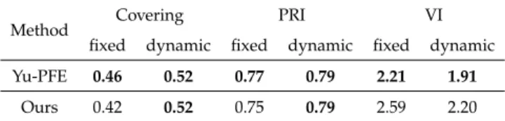
Following the strategy outlined in [27], we report results for both afixedscheme, where we run the algorithm repeatedly withkcorresponding to each number of segments in the ground-truth and average the performance across multiple runs, and adynamicscheme, where we choose the value ofkfromk=5, 10, 15, 20, 25 that yields the best performance for a particular image. The results pertaining to both of these schemes using the intensity graph construction are presented in Table (1) and the results using the gPb graph construction are presented in Table (2). From these tables, we observe that our efficient implementation of PFE yields similar covering and PRI values when compared to the implementation in Yu et al. [27] for both methods of graph construction. We note, however, that for both methods of graph construction, our VI measures were slightly higher than those reported in [27]. If we consider only the gPb graph construction, we found the standard deviation in VI values to be approximately 0.44

Method Covering PRI VI fixed dynamic fixed dynamic fixed dynamic Yu-PFE 0.46 0.52 0.77 0.79 2.21 1.91

Ours 0.42 0.52 0.75 0.79 2.59 2.20

Table 1: Comparison of Yu et al. implementation of PFE (Yu-PFE) and our efficient PFE method (Ours) on the BSDS5000 dataset using the intensity-based affinity construction. All results were averaged across images and the best results for each performance measure have been highlighted in bold.

Method Covering PRI VI

fixed dynamic fixed dynamic fixed dynamic Yu-PFE 0.45 0.56 0.78 0.81 2.26 1.77

Ours 0.43 0.51 0.74 0.78 2.30 2.04

Table 2: Comparison of Yu et al. implementation of PFE (Yu-PFE) and our efficient PFE method (Ours) on the BSDS5000 dataset using the gPb-based affinity construction [1]. All results were averaged across images and the best results for each performance measure have been highlighted in bold.

for both the fixed and dynamic schemes, with similar high deviation values for the intensity graph construction as well. If the implementation in Yu et al. [27] had high standard deviation values as well (which were not reported in their paper), it is likely that the difference in VI values between methods is not statistically significant. We will further explore the statistical significance of each of the three quantitative measures outlined here in Chapter 6.

In Figure (5), we show a plot of the computation time (in seconds), as a function of cluster number, required to compute the PFE for the 200 test images. From this figure we can see that using the intensity-based graph construction, our implementation takes anywhere between 10 seconds and 15 minutes to compute the PFE, while the gPb-based graph construction takes anywhere between 1.5 and 110 minutes to compute the PFE, depending on how many clusters are desired. The large amount of time required for the gPb-based graph construction could possibly be a result of the structure of the adjacency matrix, and could be investigated in future work. While Yu et al. [27] report that their implementation requires approximately 15 minutes to compute the PFE per image, they have not yet released code, prohibiting us from performing a direct comparison.

In this Chapter, we presented the two-stage approach outlined in [27] for approximating a solution to the PFE problem. We then outlined the computational improvements that we made to the approach and demonstrated the results of our efficient implementation based on two experiments evaluated on the BSDS500 dataset [1]. We note that at this time, code for the Yu et

0 10 20 30 40 50 60 70 80 90 100 Number of segments 101 102 103 104

Computing Time (sec)

Intensity gPb

Figure 5: Computation times for the efficient implementation of PFE based on the intensity and gPb graph constructions.

al. [27] implementation of PFE has not yet been publicly released. For this reason, our efficient implementation of PFE will be used for all experiments pertaining to the SOC algorithm for PFE approximation for the remainder of this thesis.

5

Piecewise Flat Embeddings (PFE) with Iteratively Reweighted

Rayleigh Quotients (IRRQ)

In this Chapter, we present an alternative algorithm for solving the PFE problem motivated by the Iteratively Reweighted Least Squares (IRLS) algorithms commonly used to solve`<sub>1</sub> -minimization problems [9]. In IRLS, `₁-minimization is performed by iteratively solving a succession of weighted least-squares (`₂-minimization) problems, with weights updated at each iteration to decrease the impact of large residual errors. Our new algorithm is termed Iteratively Reweighted Rayleigh Quotients (IRRQ), and, in contrast with the two-stage approach outlined in [27], it does not require an initial estimate of the data embedding, only requires the tuning of a single hyperparameter, and does not rely on a nested iterative structure.

5.1

Iteratively Reweighted Rayleigh Quotients Minimization Algorithm

To solve (3.9) subject to an orthogonality constraint, we will show that the final data embedding can be computed by iteratively solving a series of constrained weighted `<sub>2</sub>-minimization problems, with weights updated similarly to IRLS. Each constrained weighted`₂-minimization problem has the form

min Y∈Rn×k J Γ 2(Y):= n

∑

i=1 n

∑

j=1 wi,jγi,j ˆy_i−ˆy_j 2 2 (5.1) subject to: YTDY=I , YTD1=0 ,

whereΓis then×nmatrix of weights (with entriesγi,j) that is updated at each iteration.

To establish a connection between (3.9) and (5.1), we must first eliminate the balance constraint from (5.1) using the result of the following Lemma, which is proved in Appendix 8.1.

Lemma 5.1. SupposeY=D−1/2BG, whereB∈Rn×(n−1)_andG∈R(n−1)×k_{, withB=C C}T_C−1/2

, and whereCT∈R(n−1)×n_{projects vectors onto the subspace orthogonal toq=D}1/2_1/

D

1/2₁ . Then YTD1=0andYTDY=GTG.

By using this Lemma, we can solve (5.1) by first solving:

ˆ G:=arg min GT_G=IJ Γ 2 D−1/2BG , (5.2)

and then computingY=D−1/2B ˆG.

If we assume the restrictive assumption that our embedding must be one-dimensional and that none of the differences in embedding components vanish, then we can show that the

solution to (5.1) coincides with the solution to (3.9) when we choose weights according to γi,j= y ∗ i −y∗j −1

fori6=j. This proof is shown in Appendix 8.2. In practice, however, many of the component-wise differences will vanish and hence we regularize the weights as in [9]:

γi,j := h wi,j ˆy_i−ˆy_j 2 2+ε 2i−1/2 _{, (5.3)}

and we updateεaccording to the schedule prescribed by [9], which suggests:

ε←min

ε,n−1r(Y)_κ+1

, (5.4)

wherer(Y)_κ is theκthlargest element of

n wi,j ˆy_i−ˆy_j 2,∀i,j=1, . . . ,n o .

Combining the steps of solving (5.1) and updating (5.3)–(5.4) into a sequence of iterations yields Algorithm (3) for computing the PFE. Note that (5.2) can be transformed into an unconstrained minimization of the following Rayleigh quotient:

ˆ

G:=arg min trGTBTD−1/2ˆLD−1/2BG ·GTG−1

, (5.5)

where ˆLis the Laplacian of the graph having weight matrixWΓanddenotes Hadamard product. Since (5.1) is equivalent to (5.2) and (5.2) can be transformed into an unconstrained minimization of a Rayleigh Quotient, we term this algorithmIteratively Reweighted Rayleigh Quotient(IRRQ) Minimization.

In contrast with the SOC algorithm, IRRQ requires the tuning of only a single hyperparamter,

κ, and it guarantees a solution in which the orthogonality constraint is strictly enforced.

Furthermore, IRRQ does not require an initial estimate of the final data embedding. With an initial set of unit weights, IRRQ can be thought of as being implicitly initialized with the solution to the relaxed NCut problem, sinceJ11T

2 (Y)is equivalent to the LE objective function

J2(Y) in (3.7). If different initializations are desired, for instance, by computing an initial embeddingY(0)using a Gaussian Mixture Model as in [27], these can be incorporated by setting the initial weightsγ(_i,0_j)=

ˆy (0) i −ˆy (0) j −1 2 orγ (0) i,j = wi,j ˆy (0) i −ˆy (0) j 2 2+ε 2 0 −1/2 .

5.2

Solving Step (a) of the IRRQ Algorithm

The computation to be done in step (a) of Algorithm (3) is non-trivial. From the relationship between (5.1)–(5.2), we can see that computingY(m+1)is equivalent to solving

ˆ G(m+1):=arg min GT_G=IJ Γ(m) 2 D−1/2BG (5.6)

Algorithm 3IRRQ Minimization Algorithm for PFE

procedureIRRQ(W,k,κ)

γ(_i,0_j):=1,ε0:=1,m:=0,n:=size(W, 1)

whileεm >0do

(a)Y(m+1):=arg min YT_DY=I YT_D1=0 Y∈Rn×k J₂Γ(m)(Y) (b)εm+1:=min εm,n−1r Y(m+1) κ+1 (c)γ(_i,m_j+1):= h wi,j ˆy_i−ˆy_j 2 2+ε 2 m+1 i−1/2 end while return Y(m) end procedure

and then computingY(m+1)=D−1/2B ˆG(m+1). The problem posed in (5.6) can be expressed as the following Rayleigh quotient minimization:

ˆ

G(m+1):=arg min trGTBTD−1/2ˆL(m)D−1/2BG ·GTG−1

, (5.7)

where ˆL(m) _{is the Laplacian of the graph having weight matrix WΓ}(m) _{and denotes}

Hadamard product. The solution to (5.7) is given byGˆ(m+1) = UH, whereU ∈ R(n−1)×k _is

the matrix whose columns are the orthonormal eigenvectorsu1, . . .,ukcorresponding to the

smallest eigenvalues ofBTD−1/2ˆL(m)D−1/2B, andH∈Rk×k_{is an arbitrary orthogonal matrix.}

(Note that by eliminating the balance constraint, we also eliminate the possibility of a trivial eigenvalue ofBTD−1/2ˆL(m)D−1/2B. Such an eigenvalue would have eigenvectorpfor which

Bpis in the direction ofq; however, this is contradicted by the fact that range(B) =range CT

.)

In order for this solution to scale to largen, we must consider the structure ofC, and whether or not the matrixBmust explicitly be constructed. Since we have the ability to choose anyC

such thatCTprojects vectors onto the subspace orthogonal toq, we chooseCT= [ˆq| −q1In−1], where ˆq = [q2,q3, . . . ,qn]T and In−1 is the(n−1)×(n−1) identity matrix. This particular choice ofCis sparse, and therefore, as shown in Appendix 8.3, the multiplication of an arbitrary vector byBTD−1/2ˆL(m)D−1/2Bcan be performed efficiently without explicitly constructingB. Finally, we note that the solution to step (a) is not unique: postmultiplyingY(m+1)byHT, where

H is orthogonal, still produces a valid solution. This does not pose a problem for steps (b) and (c) of Algorithm (3) sincerandγi,j are invariant to such transformations ofY(m+1). As a

consequence, IRRQ minimization could yield an entire family of solutions to the PFE problem, which could be problematic since the`<sub>1</sub>-norm is not invariant under orthogonal transformations. In practice, however, we have found that the`1-norm is minimized for the choiceH=Iand, as such, we suggest this choice. Proof that this is the best choice remains an open problem.

5.3

Choosing

κ

for Rapid Convergence

Linear convergence in IRLS algorithms for`1-minimization can typically be achieved ifκ is

chosen large enough so that if the solution isθ-sparse, thenκ > θ. We note that there are

more sophisticated convergence results provided in [9], but this is a good rule-of-thumb. While proving convergence results for the IRRQ algorithm remains an open problem, we use a similar strategy to [9] in choosingκ. In practice, the main difficulty in choosingκis thatθis not known

exactly until the problem is solved. To approximateθ, we use an estimate ˆθequal to twice the

number of graph edges that connect different clusters from ak-means clustering performed on the initial embeddingY(0).

To provide “scale-free” behavior, we introduce the hyperparameter ˜κ that can be selected in

(0, 1). ˜κ can then be mapped toκ by κ = θˆ+κ˜ 2|E| −θˆ, where |E| is the total number of

6

Segmentation Experiments and Results

In this Chapter, we provide an overview of the experiments we conducted to test the relative performance of both CCNCut and NCut minimization and to compare the SOC and IRRQ algorithms on the task of image segmentation. We then provide results from these experiments and explore the benefits and limitations of the two algorithms.

6.1

Segmentation Experiments

To compare the performance of CCNCut and NCut minimization, as well as to compare the relative performance of the SOC and IRRQ algorithms for CCNCut minimization, we use these algorithms to segment the 200 test images in the BSDS500 dataset [1]. This dataset contains a variety of manually-labeled segmentations with varying numbers of segments that can be used as ground truth. Similar to the experiments we conducted in Chapter 4, we construct two types of graphs for each image. We first downsample the image by a factor of four and then compute either the intensity differences across pixels within a four-pixel neighborhood of one another based on the 4-nearest neighbor algorithm, or compute the globalized probability of boundary (gPb) at each pixel using the code provided with the BSDS500 dataset.

For each of the algorithms, we segment each image multiple times, once for eachk(number of segments) value reflected in the ground truth and once for eachk=5, 10, 15, 20, and 25 not reflected in the ground truth. Each segmentation algorithm proceeds by computing the desired data embedding (LE or PFE) and then performingk-means clustering on the final embedding to assign discrete labels to each pixel.

For CCNCut minimization using the SOC algorithm, we test segmentation performance based on two different initializations. The first is based on the Laplacian Eigenmaps (LE) algorithm and the second is based on the Gaussian Mixture Model (GMM) as in [27]. These two initialization schemes are labeled as C-SOC-L and C-SOC-G respectively in our experimental results. For both initialization methods, we perform the two-stage approach outlined in [27]. Unless otherwise stated, in stage one, we set the maximum number of outer iterations to 10 and the maximum number of inner iterations to 5 with hyperparameters λ = 10, 000 and r = 100.

Unless otherwise stated, in stage two, we set the maximum number of inner iterations to 100 with hyperparametersλ=10, 000 andr=10. All of these parameter choices are the same as in

[27].

based on two different weight initialization schemes. The first is our default scheme where all weights are initialized to unity (implicit LE initialization of PFE) and the second is a scheme where weights are initialized according to embeddings formed from a GMM. These two initialization schemes are labeled as C-IRRQ and C-IRRQ-G respectively in our experimental results. In both initialization schemes, unless otherwise stated, the maximum number of iterations is 20, and the hyperparameter ˜κ is set to 0.02. The seed for the random number

generator is reset before every initialization, ensuring that the same GMM’s are used to initialize the C-SOC-G and C-IRRQ-G algorithms.

6.2

State-of-the-Art on BSDS500

Although Yu et al. [27] held state-of-the-art results on the BSDS500 dataset at the time of their publication in 2015, we must note a few key points. First, the state-of-the-art results published in [27] were based on the contour-driven hierarchical segmentation schemes presented in [1] and [2]. While the hierarchical schemes were not used in this thesis for discrete labeling, we believe these clustering strategies would be interesting to explore in future work for both the SOC and IRRQ algorithms. Second, in 2016, [7] developed a scheme to better align hierarchical data partitions based on depth and scale that produced comparable results to those presented in [27].

In 2016, Zhao and Griffin [29] utilized multi-level cues and semantic predictions from a Fully Convolutional Neural Network (FCNN) [14] to build an image segmentation scheme based on a bottom-up approach. At the time of writing this thesis, the results presented in [29] hold state-of-the-art on the BSDS500 dataset. Table (3) shows the results from [7, 27, 29] to give the reader an understanding of current state-of-the-art segmentation covering, PRI, and VI values on the BSDS500 dataset. In the table, there are two results reported for each quantitative measure: Optimal Dataset Scale (ODS) and Optimal Image Scale (OIS) [1]. ODS and OIS provide two different approaches for generating a single segmentation of an image, based on the use of hierarchical clustering techniques.

6.3

Results

Figures (6) and (7) demonstrate segmentation results for various images from the BSDS500 dataset, each chosen for specific values ofkbased on the gestalt sense of the image provided by the segmentation. Figure (8) demonstrates C-IRRQ segmentation results for varying cluster numbersk.