Current and future intensity-duration-frequency curves based on weighted ensemble GCMs and temporal disaggregation

http://dx.doi.org/10.17576/jsm-2020-4910-03

Current and Future Intensity-Duration-Frequency Curves based on Weighted

Ensemble GCMs and Temporal Disaggregation

(Lengkung Keamatan-Tempoh-Frekuensi Semasa dan Masa Hadapan berdasarkan Pemberatan GCM Ensembel dan Pengasingan Temporal)

NURADDEEN MUKHTAR NASIDI*, AIMRUN WAYAYOK, AHMAD FIKRI ABDULLAH & MUHAMAD SAUFI MOHD KASSIM

INTRODUCTION River

ABSTRACT

Hydrological events are expected to increase in both magnitude and frequency in tropical areas due to climate variability. The Intensity – Duration – Frequency (IDF) curves are important means of evaluating the efficiency of irrigation and

drainage systems. The necessity to update IDF curves arises from the need to gain better understanding of the impacts of climate change. This study explores an approach based on weighted Global Circulation Models (GCMs) and temporal disaggregation method to develop future IDFs under Representative Concentration Pathways (RCP)

emission scenarios. The work consists of 20 ensemble GCMs, three RCPs (2.6, 4.5, and 8.5) and two projection periods (2050s and 2080s). The study compared three statistical distributions and selected Generalized Extreme Value

(GEV) being the best fitting distribution with baseline rainfall series and therefore used for IDF projection. The result obtained shows that, the highest rainfall intensities of 19.32, 35.07 and 39.12 mm/hr occurred under 2-, 5-, and 20 years return periods, respectively. IDFs from the multi-model ensemble GCMs have shown increasing intensity in the future for all the return periods. This study indicated that the method could produce promising results which can be extended to other catchments.

Keywords: Cameron Highlands; climate change; flooding; HYETOS; soil erosion ABSTRAK

Kejadian hidrologi dijangka meningkat pada magnitud dan kekerapan di kawasan tropika kerana perubahan iklim. Lengkung Keamatan-Tempoh-Frekuensi (IDF) ialah kaedah penting untuk menilai kecekapan sistem pengairan dan saliran. Keperluan untuk mengemas kini lengkung IDF timbul daripada keperluan untuk mendapatkan pemahaman yang lebih baik mengenai kesan perubahan iklim. Kajian ini meneliti pendekatan berdasarkan pemberatan Model Peredaran Global (GCM) dan kaedah tidak pengagregatan secara temporal untuk memajukan IDF masa hadapan di bawah senario pelepasan Laluan Konsentrasi Perwakilan (RCP). Karya ini terdiri daripada 20 GCM ensembel, tiga

RCP (2.6, 4.5 dan 8.5) dan dua tempoh unjuran (2050-an dan 2080-an). Kajian ini membandingkan tiga taburan statistik dan Nilai Ekstrim Umum (GEV) terpilih sebagai taburan yang paling sesuai dengan garis tapak siri curahan hujan. Oleh itu, ia digunakan untuk unjuran IDF. Hasil yang diperoleh menunjukkan bahawa keamatan curahan hujan tertinggi ialah 19.32, 35.07 dan 39.12 mm/jam dan masing-masing berlaku dalam jangka masa pengembalian 2-, 5- dan 20 tahun. IDF daripada multi-model GCM ensembel telah menunjukkan peningkatan keamatan pada masa hadapan untuk semua tempoh pengembalian. Kajian ini menunjukkan bahawa kaedah tersebut dapat menghasilkan keputusan yang menggalakkan serta dapat diaplikasikan ke kawasan tadahan curahan hujan yang lain.

Kata kunci: Banjir; hakisan tanah; HYETOS; perubahan iklim; Tanah Tinggi Cameron

INTRODUCTION

The impact of climate change on extreme rainfall has received a great deal of attention in few decades because the climate change affects society, economy, and environment.

Global warming has gradually increased with a steady increase in global average temperatures over the last three decades (Zhiying & Fang 2016). Global warming induces irregular weather events, and significant changes in the frequency and intensity of extreme rainfall have been

. , observed over the past decades. Existing studies have shown that as warmer climates increase water vapor, precipitation, and the risk of increasing flooding (IPCC 2013). Some reports warn that although the effects of climate change cannot be accurately predicted, an increase in rainfall variability raises the risk of more frequent and more severe extreme precipitations events (Choi et al. 2019; Gericke et al. 2019).

Observations on a global scale have shown that the frequency and intensity of extreme events have significantly changed over the last decades (Perkins et al. 2012). Irregular changes in extreme precipitation have been reported regardless of changes in annual and seasonal precipitations (Araji et al. 2018). Moreover, on a regional scale, several studies in Southeast Asia have shown a rise in the rate of heavy rainfall over recent decades (Choi et al. 2019). Several areas of application, such as overall risk assessments or the design of flood protection systems, require reliable precipitation statistics with high spatial resolution, including estimates for events with high return periods (Ehmele & Kunz 2019). The GCMs datasets are obtainable from the Fifth Assessment Report (AR5) of the Intergovernmental Panel on Climate Change (IPCC) (IPCC 2013). Although, the uncertainty inherently possessed by each GCM is significant (Mandal et al. 2016; Mondal et al. 2017), the multi-model ensemble approach is recommended by many existing studies to improve accuracy of climate impact assessments (Amanambu et al. 2019).

Rainfall in Malaysia is usually received using a daily rain gauge available at weather stations across the country. To develop IDF curves, rainfall data are often needed at a finer scale, such as hourly rather than daily scale. The temporal disaggregation method have been used to reduce large scale temporal series, usually daily or monthly to small scale sub daily series (Koutsoyiannis & Onof 2001; Kristvik et al. 2019). One of the challenges of urban drainage modeling is that IDFs with a short duration are required due to the corresponding concentration time within the catchment area. Therefore, disaggregation has recently become a major technique for hydrological modeling of rainfall time series. This study applied temporal disaggregation method to obtain hourly rainfall series from the available daily time series. Future climate shows high extremes for hydrological events particularly at tropical regions with consequences of frequent unexpected flooding (Song et al. 2019).

Severe flood events resulting from heavy rainfall over large areas have the potential to cause huge economic losses of billions Ringgit (MYR) in Malaysia. The recent most devastating flood incident in Malaysian occurred in 2004 which claimed 64 lives with economic

loss of about 480 million USD (D-iya et al. 2014). The main causes of this disaster were identified as problems associated with drainage systems and high unusual rainfall amount. Similarly, the study reported that, 45% of entre river basins of Malaysia are vulnerable to recurrent floods, with estimated 9% of Malaysia under considerable risk of flood disaster. Furthermore, there were occurrences of mud flows in Cameron Highlands due to high frequency of extreme rainfall events. For example, the mud flow that occurred in 2014 killed at least three people, injured five people and necessitated evacuation of 90 victims to the relief center at Ringlet settlement (Abdullah et al. 2019). Thus, there is urgent need to adjust the design calculations to reflect the actual Malaysian present conditions.

Consequently, this study aimed to develop current and future IDF curves using multi-model ensemble climate models and temporal disaggregation at Cameron Highlands watershed. The study compared three statistical distributions to select the best one fits with current rainfall series for generating future IDF curves. Thus, the outcome of this study can be replicated in other areas with similar climate and would provide useful information for management to make adequate preparations.

MATERIALS AND METHODS STUDY AREA

Cameron Highlands is located at the Pahang State of Peninsular Malaysia situated on 4o_{28’N, and 101°23’E}

with average temperatures of 24and 14 ℃ during the day and night, respectively (Figure 1). The elevation ranges between 187 and 2067 m above mean sea level with average annual precipitation of 2660 mm (Abdullah et al. 2019; Razali et al. 2018). This region has two distinctive peaks periods of monthly rainfall with first peak rainfall observed in April while the second with higher rainfall volume in November (Abdullah et al. 2019). The highlands are regarded as a vital hill stations for the country which occupies an area of 712.18 km2_.

Moreover, the area is surrounded by Kelantan and Perak from north and west, respectively, and has a potential for growing a wide variety of vegetables, flowers, and other ornamental plants. The excellent climatic condition in the highlands provides opportunity for agricultural activities as the main business and attracts many tourists from all over the globe (Gasim et al. 2012; Razali et al. 2018). The study flow chart is presented in Figure 2 showing major activities involved for the IDF curves development.

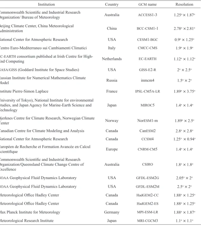
GLOBAL CIRCULATION MODELS AND FUTURE SCENARIOS In this study, the GCMs data were accessed from World Climate Data Center (https://cera-ww.dkrz.de/WDCC/ ui/cerasearch) under Fifth Assessment Report (AR5)

of Intergovernmental Panel on Climate Change (IPCC) (Table 1). The projections were conducted under three emission scenarios; RCP2.6, RCP4.5, and RCP8.5 and two projection periods (2050s and 2080s). The scenarios represent low, medium, high, and very high greenhouse FIGURE 2. Study flow diagram for the major activities

gas emission levels, respectively (Araji et al. 2018). In addition, the data source contains GCMs outputs of the Coupled Model Intercomparison Project Phase 5 (CMIP5) archive with both historical and future projected climate data on global scale. In this study, thirty years’ historical data (1976-2005), is defined as baseline climate while the multiplicative delta change statistical method is applied

for bias correction. The GCM data are in a form of grids as shown in Table 1, and the lower the degree indicates high resolution. Normally, interpolation is required to get the exact climate data for a specific location of interest. This work obtains the GCMs datasets by supplying appropriate coordinates of the study area during the process downscaling.

TABLE 1.Atmospheric global circulation models (GCMs)

Institution Country GCM name Resolution

Commonwealth Scientific and Industrial Research

Organization/ Bureau of Meteorology Australia ACCESS1-3 1.25o × 1.87o Beijing Climate Center, China Meteorological

Administration China BCC-CSM1-1 2.78o×2.81o

National Center for Atmospheric Research USA CESM1-BGC 0.9o _{× 1.25}o Centro Euro-Mediterraneo sui Cambiamenti Climatici Italy CMCC-CMS 1.9o_{× 1.9}o EC-EARTH consortium published at Irish Centre for

High-End Computing Netherlands EC-EARTH 1.12o× 1.12o

NASA/GISS (Goddard Institute for Space Studies) USA GISS-E2-R 2o_{× 2.5}o Russian Institute for Numerical Mathematics Climate

Model Russia inmcm4 1.5o× 2o

Institute Pierre-Simon Laplace France IPSL-CM5A-LR 1.89o_{× 3.75}o University of Tokyo), National Institute for environmental

Studies, and Japan Agency for Marine-Earth Science and

Technology Japan MIROC5 1.4

o_{× 1.4}o Bjerknes Centre for Climate Research, Norwegian Climate

Center Norway NorESM1-m 1.89o× 2.5o

Canadian Centre for Climate Modeling and Analysis Canada CanESM2 2.8o_{× 2.8}o National Center for Atmospheric Research Canada CCSM4 1.25o _{× 0.94}o Européen de Recherche et Formation Avancée en Calcul

Scientifique Europe CNRM-CM5 1.4o×1.4o

Commonwealth Scientific and Industrial Research

Organization/Queensland Climate Change Centre of

Excellence Australia CSIRO 1.8

o_{× 1.8}o NOAA Geophysical Fluid Dynamics Laboratory USA GFDL-ESM2G 2.05o_{× 2}o NOAA Geophysical Fluid Dynamics Laboratory USA GFDL-ESM2M 2.5o_{× 2}o Meteorological Office Hadley Center Canada HadGEM2-CC 1.88o_{× 1.25}o Meteorological Office Hadley Center Canada HadGEM2-ES 1.88o_{× 1.25}o Max Planck Institute for Meteorology Germany MPI-ESM-LR 1.88o_{× 1.87}o Meteorological Research Institute Japan MRI-CGCM3 1.1o_{× 1.1}o

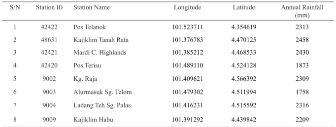
RAINFALL STATIONS AND GCMS DOWNSCALING METHOD The work uses of thirty years observed rainfall data on daily basis from eight metrological stations within the study watershed (Table 2). The data was obtained from department of Drainage and Irrigation Drainage (DID) Malaysia. Two stations (Alurmasuk Sg. Telom and Pos Terisu) have missing data for about three month each. Thus, the missing data was filled by taking average of rainfalls recorded from nearest neighboring stations (Hanaish et al. 2011; Koutsoyiannis & Onof 2001) two case studies (from the UK and US. Highest annual

rainfall amount of 2458 mm was recorded at Kajiklim Tanah Rata whereas the lowest amount (1758 mm) was received at Alurmasuk Sg. Telom rainfall stations.

Moreover, downscaling of the climate data was done by change factor method which entails several steps to estimate the empirical cumulative distribution functions (CDFs) for future GCM (GCM_f) and baseline (GCM_b) for all the emission scenarios. For the detail procedure of downscaling using change factor method, the reader may refer to (Anandhi et al. 2011).

TABLE 2. Metrological stations and the corresponding observed rainfall data

S/N Station ID Station Name Longitude Latitude Annual Rainfall

(mm)

1 42422 Pos Telanok 101.523711 4.354619 2313

2 48631 Kajiklim Tanah Rata 101.376783 4.470125 2458

3 42421 Mardi C. Highlands 101.385212 4.468533 2430

4 42420 Pos Terisu 101.489110 4.524128 1873

5 9002 Kg. Raja 101.409621 4.566392 2309

6 9003 Alurmasuk Sg. Telom 101.479302 4.511994 1758

7 9004 Ladang Teh Sg. Palas 101.416231 4.515592 2316

8 9009 Kajiklim Habu 101.391292 4.439842 2209

WEIGHTED MEANS ENSEMBLE OF GCMS

The method of weighted ensemble GCMs has been practiced by Araji et al. (2018) and it gave promising results, because it improves accuracy of the climate projection. It is believed that this approach ensures minimum level of uncertainty inherently contained in the global models. Since, each GCM can project different future climate variables, which indicates the gross uncertainty associated with the climate models (Araji et al. 2018). Thus, it is agreed that weighted ensemble means can help to make stronger projection taking into consideration, the contribution of each model studied. In this study, the weight given to each GCM was based on mean deviation between simulated and observed monthly values of precipitation from the baseline period (1976-2005). Therefore, GCMs with greater weight predicts climatic values with more accuracy in the future. The equation (1) was used for weight determination of individual GCM with each climate scenario (Araji et al. 2018)

(1)

where W_i is the weight of each model in month i and ΔP_{i, j} is the difference between average of precipitation simulated j in month i of the baseline period (1976-2005) from the corresponding observed data in the same period.

To establish climate change scenarios, Equation (6) was applied to the average of 30 years future periods; (2040-2069) and (2070-2099) for each climate model and its corresponding simulated baseline period (1976-2005). Also, in order to generate mean weighted ensemble GCMs, Equations (2) and (3) were applied to the scenario files with different GCMs and emission scenarios, that are RCP2.6, RCP4.5, and RCP8.5 emission scenarios,

(2)

(3)

where Pi is climate change scenarios related precipitation for month i (1< i <12); P̅is the simulated future and historical average precipitation of 30 years, derived from each climate model for month I, P_i,j and W_{i j} are obtained

Wi = (_∆Pi,j1 ) ∑ (n _∆Pi,j1 ) j=1 Pi= _{P̅GCM baseline,i}P̅GCM Future,i

E = ∑ Pni=1 i,j× Wi,j

Pi= _P̅P̅_{GCM baseline,i}GCM Future,i

from Equations (5) and (6), n is the number of climate models, and E represents mean ensemble GCMs.

DISAGGREGATION OF MONTHLY RAINFALL TO HOURLY TEMPORAL SCALE USING HYETOS

Hyetos is based on the Bartlett - Lewis Rectangular Pulse (BLRP) process theory that has been built into a computer program. This is a validated disaggregation technique that changes larger scale data to obtain finer scale data without affecting the stochastic structure of the model (Koutsoyiannis & Onof 2001). The fundamental assumptions of the model are: the origin of the storm after the Poisson process (rate lambda-λ), the origin of the cells of each storm after the Poisson cycle (rate beta-β), the arrival of each storm after the exponentially distributed time (parameter gamma-γ), the length of each cell is exponentially distributed (parameter eta-η), and each cell has a uniform intensity with a defined distribution (exponential or gamma). The parameter η is uniformly varies from storm to storm with a gamma distribution with the form parameter alpha-α and the scale parameter v. Subsequently, the parameters β and γ also differ in such a way that the ratios k = β/η and φ = γ/η remain constant. The distribution of the Xij uniform intensity is usually considered to be exponential with the 1/μX parameter. Hyetos adopts the Bartlett-Lewis model for the generation of synthetic precipitation along with an adjustment protocol to keep consistency with the daily data observed. For a wet-day sequence, the model runs many times and produces a sequence that best matches the daily data observed. The series of synthetic hourly rainfall is adjusted according to the proportional adjustment process, which is aggregated to the daily data, in such a way that certain statistics are preserved between daily and hourly data (Liew et al. 2014). In addition to the adjustment process, the model uses repetition to ensure consistency between observed and modeled results. For longer series, the model divides the wet series into different clusters separated by at least one day, minimizing the computational time. The model runs separately for each wet cluster series until the departure of the sequence of daily amounts from the specified sequence of daily rainfall is lower than the acceptable limit (Equation 4). For the sequence of L wet days produced, the daily precipitation depths are computed and compared to the observed precipitation depths by logarithmic distance, which is mathematically indicated as (Koutsoyiannis & Onof 2001),

(4) where Z_i and Z_i are observed and generated daily rainfall depth of day i of wet day sequence, respectively; and c is

constant (= 0.1 mm). The model verifies if departure d is smaller than acceptable limit da, which continues for the allowed number of repetitions and if the condition is not satisfied, the cell is discarded and new one is generated.

CREATING INTENSITY–DURATION–FREQUENCY (IDF) CURVES

There are several distribution functions for IDF analysis: Extreme Value Type I, i.e., Gumbel (EVI) distribution, Generalized Extreme Value (GEV) distribution, Gamma distribution, Log Pearson III distribution, Lognormal distribution, Exponential distribution, and Pareto distribution, Example (Shrestha et al. 2017) and GEV distribution, example (Choi et al. 2019; Shrestha et al. 2017), are the most commonly used function for IDF analysis. In this present work, the annual maximum series of observed rainfall data (1976-2005) is integrated into the distributions of GEV, Gamma and Gumbel using moment and L-moment methods. The mathematical expression for GEV probability distribution is Equation (5).

(5) where k (shape parameter); σ (scale parameter, σ > 0) and µ (location parameter) are to be determined. For k = 0, GEV reduces to Gumbel (EVI) distribution and for k < 0, it reduces to Extreme Value Type I distribution, which implies an upper bound of the variable, which is not the case in maximum rainfall intensity.

The method of L-moments, first introduced by Karl Pearson in 1902, considers that the good estimates of the parameters of the probability distribution are those for which the moments of the probability density function of the origin are equal to the corresponding moments of the sample data (Chow et al. 1988). L-moments are enhancements over traditional moments, which have a major advantage, being the linear functions of the data, are less influenced by the effects of sampling variability and are more resilient than standard data outlier moments. It is also less prone to error in estimation and allows for more accurate inferences from small samples on the underlying probability distribution (Hosking 1990; Shrestha et al. 2017).

Let X_1:n ≤ X_2:n ≤ . . . ≤ X_n:n be the order statistics of the random sample size n from the distribution X, and X is the real random variable measured with the cumulative distribution function F(x), the L-moments can be calculated using Equation (6).

(6) r = 1, 2. . ., where the EX_{j: r} and can be expressed as in Equation (7). d = [∑ ln (Zi+c Z̃i+c) 2 L i=1 ] 1/2 𝐹𝐹(𝑥𝑥) = exp⁡ [−⁡(1 − 𝑘𝑘𝑥𝑥−𝜇𝜇_𝜎𝜎 )1/𝑘𝑘] λr= r−1∑r=1k=0(−1)k(r − 1_k )EXr−k:r

(7) For more details of L-moments and parameters for various probability distributions, the readers may refer to Hosking and Wallis (1997). For the selection of distribution functions, the fitness of the probability distributions is performed by a comparative test of the theoretical and sample values of the relative frequency or cumulative frequency function, using the Chi-Squared test to determine whether the annual maximum rainfall data is compatible with the defined distribution.

VALIDATION OF THE SIMULATED PRECIPITATION The Root Mean Square Errors (RMSE) and Efficiency Index (EI) have been used as standard metrics to show that the model can reproduce past rainfall (Shrestha & Jetten 2018). RMSE and EI are mathematically expressed in Equations (8) - (10), (8) (9) (10) where X_i is observed data at time i;

RMSE = √1_n∑ (Xni=1 i− Yi)2 (8)

EI =∑ (Xni=1 i − X̅ )2−∑ (Xni=1 i−Yi)2

∑ (Xni=1 i−X)̅̅̅2 (9)

𝑋𝑋

̅is mean of observed =1_𝑛𝑛∑𝑛𝑛𝑖𝑖=1𝑋𝑋𝑖𝑖 (10)

data; Yi is synthetic data at time i; and n is the total number of data points. The RMSE for both mean and maxima are in acceptable range and further EI is greater than 90% for the two projected rainfall datasets.

The procedure for the IDF development and making future Projection has been described by Singh and Panda

(2017). The method involves extracting climate models, downscaling to finer resolutions, extreme value analysis, and IDF curve development. The IDF curves explains the relationship between rainfall intensity, rainfall duration and return period (inverse of its probability of exceedance). Moreover, IDF curves are obtained through frequency analysis of rainfall observations commonly used in the design of hydrologic, hydraulic, and water resource systems.

RESULTS AND DISCUSSION

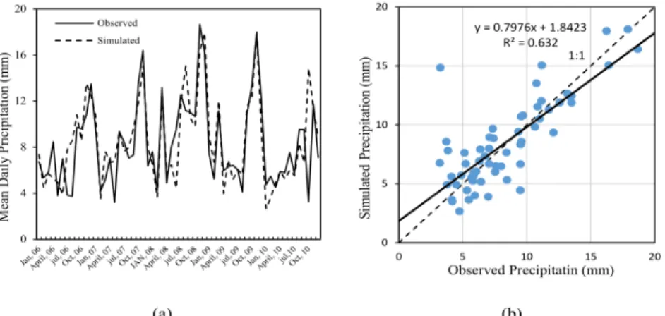
PERFORMANCE OF THE MULTI-MODEL ENSEMBLE GCMS In this study, both observed and simulated rainfall series are compared for the periods of five years testing datasets starting from January 2006 to December 2010 (Figure 3). This indicates the uniformity and consistency between observed and simulated rainfall series (Nkunzimana et al. 2019). The peak observed daily rainfall of 18.4 mm is observed in October 2018 while the least of 3.8 mm occurred in January 2017 (Figure 3(a)). Similarly, the simulated precipitation follows the same patterns as that of the observed throughout the testing period, except in July 2010 where discrepancy of 4.8 mm is recorded. Moreover, the comparison between the two datasets showed 63.2% coefficient of determination and form a linear distribution around 1:1 straight line (Figure 3(b)). The outcome showed that, RMSE and EI for the simulated model are 19.7 and 0.91 for 2050s, and 12.5 and 0.94, respectively. Moreover, fifteen years observed mean daily precipitation data. During the validation period, highest mean daily precipitation of about 18.6 mm was recorded for both observed and simulated precipitations (Figure 3(b)). This relationship shows a good distribution pattern of rainfall for the period of performance assessment. Thus, the performance of this model during testing period shows its capability to predict future precipitation.

𝐸𝐸𝐸𝐸𝑗𝑗:𝑟𝑟= _{(𝑗𝑗−1)!(𝑟𝑟−𝑗𝑗)!}𝑛𝑛! ∫𝑥𝑥{𝐹𝐹(𝑥𝑥)}𝑗𝑗−1{1 − 𝐹𝐹(𝑥𝑥)}𝑟𝑟−𝑗𝑗𝑑𝑑𝐹𝐹(𝑥𝑥)

RMSE = √1_n∑ (Xni=1 i− Yi)2 (8)

EI =∑ (Xni=1 i − X̅ )2−∑ (Xni=1 i−Yi)2

∑ (Xni=1 i−X)̅̅̅2 (9)

𝑋𝑋̅=1_𝑛𝑛∑𝑛𝑛𝑖𝑖=1𝑋𝑋𝑖𝑖 (10)

RMSE = √1_n∑ (Xni=1 i− Yi)2 (8)

EI =∑ (Xni=1 i − X̅ )2−∑ (Xni=1 i−Yi)2

∑ (Xni=1 i−X)̅̅̅2 (9)

𝑋𝑋̅=1_𝑛𝑛∑𝑛𝑛𝑖𝑖=1𝑋𝑋𝑖𝑖 (10)

FIGURE 3. Performance of ensemble GCMs (a) during calibration (b) comparing observed vs simulated precipitations

STATISTICAL DOWNSCALLING

In this study, the multi-model ensemble GCMs projects future rainfall variations in two periods of the same length within 21st century. The periods are 2040-2069 and 2070-2099 which were represented in this study as 2050s and 2080s for simplicity. All the future scenarios are downscaled at mean daily scenarios and then disaggregated to hourly forms. Moreover, the weighted average of the ensemble means of 20 GCMs projection is aimed to supply an average change of the rainfall distribution patterns projected at the study location.

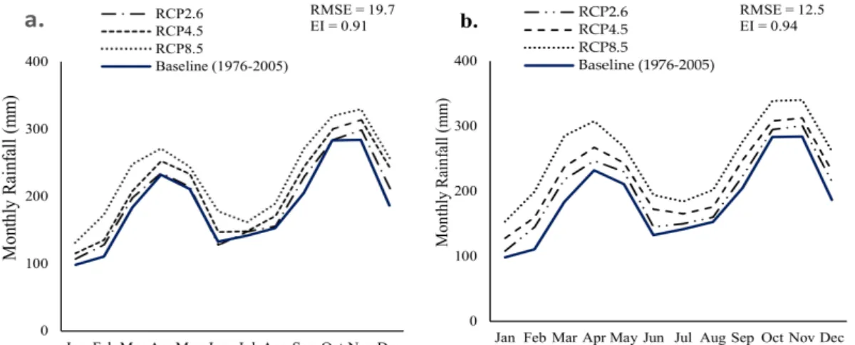
Figure 4 shows the rainfall distribution patterns for

2050s and 2080s for baseline and projection scenarios. In this period, the amount of projected rainfall for all the emission scenarios has been increased to at least 30% compared to baseline conditions. However, there is no considerable changes found among the scenarios in June and September. Conversely, there is noticeable increment of projected rainfall volumes particularly in both November and December where the ensemble GCMs predicted in the range of 9 and 20% increments, respectively. Moreover, during March, changes of projected rainfalls were observed, except that RCP4.5 have the same projection patterns (Figure 4(a)).

In 2080s projection, the ensemble model predicts substantially higher rainfall distribution patterns when compared to 2050s projection, where all the scenarios projected volume of rainfall relatively above the baseline (Figure 5(b)). In this period, we found that, there is more distinctive variations of projected rainfalls among the emission scenarios. For example, there are 7, 12, and 29% more rainfall in January under RCP2.6, RCP4.5, and RCP8.5 relative to baseline climate, respectively. However, it is seen that RCP2.6 scenario projects slightly above current rainfall amounts for both 2050s and 2080s periods. This can be explained by the fact that, RCP2.6 scenario assumes that, stringent measures are applied in the release of greenhouse gases which is a factor responsible for climate variability (IPCC 2014).

Another noticeable change in rainfall amount occurs during October and November where all the scenarios produced distinctly high rainfall amounts. The RCP8.5 emission scenario projects high volume of rainfall of more than 20% from baseline which may be unsafe for the watershed drainage systems, unless adequate measures are put in place. This shows an increasing trend of potential soil

FIGURE 4. Future precipitation relative to baseline (1976-2005):

(a) for 2050s projection, (b) for 2080s projection

erosion due to climate change and could be more severe toward the end of 21st century.

GENERATING FUTURE IDF CURVES FROM DISAGGREGATED SUB-DAILY PRECIPITATION

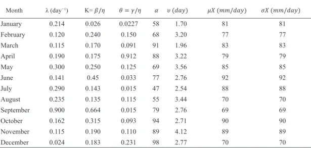
The approach is based on the assumption of the BLRP process that can be extracted from the expressions described by the parameters - λ, k, φ, α, v, µX and σX that mathematically elucidate the event of precipitation. The purpose of this approach was to maintain statistical characteristics such as mean, and variance of the time series observed with the synthetically generated disaggregated time series. The calculation of the BLRP parameters was made by measuring the statistical characteristics of the 3, 12 and 24 h observed data for each month from 1976 to 2006 separately (Figure 5). The timeline between 1976 and 2006 was chosen for analysis as the maximum daily rainfall occurred during the same period. To minimize the relative error between the synthetic and the observed values, the parameters λ, k, φ, α, v, µX and σX were optimized.

FIGURE 5. Means of rainfall distribution for various durations

Similarly, Figure 6 shows the variance of monthly time series during calibration for both historical and simulated precipitations. Moreover, Table 3 presents

Modified Bartlett-Lewis Parameters for rainfall disaggregation to hourly scales.

FIGURE 6. Varians of rainfall distribution for various durations

TABLE 3. Modified Bartlett-Lewis parameters

January 0.214 0.026 0.0227 58 1.70 81 81 February 0.120 0.240 0.150 68 3.20 77 77 March 0.115 0.170 0.091 91 1.96 83 83 April 0.190 0.175 0.912 88 3.22 79 79 May 0.300 0.250 0.125 69 3.56 85 85 June 0.141 0.45 0.033 77 2.76 92 92 July 0.290 0.143 0.015 47 2.54 88 88 August 0.235 0.135 0.115 55 3.44 70 70 September 0.900 0.664 0.015 79 2.76 69 69 October 0.162 0.315 0.093 94 2.71 90 90 November 0.115 0.190 0.110 89 4.12 89 89 December 0.024 0.183 0.231 98 2.77 70 70

GENERATION OF FUTURE IDF CURVES

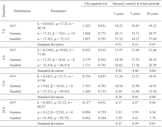
In this study, the annual maximum rainfalls at different durations from 1976 to 2005 were fitted into Generalized extreme value (GEV) distribution, Gamma distribution, Gumbel distribution. Chi-squared (χ2) test results showed the GEV distribution fits better than both Gamma and Gumbel for all the annual maximum rainfall durations (Table 4). Similarly, the Gamma fits better than Gumbel

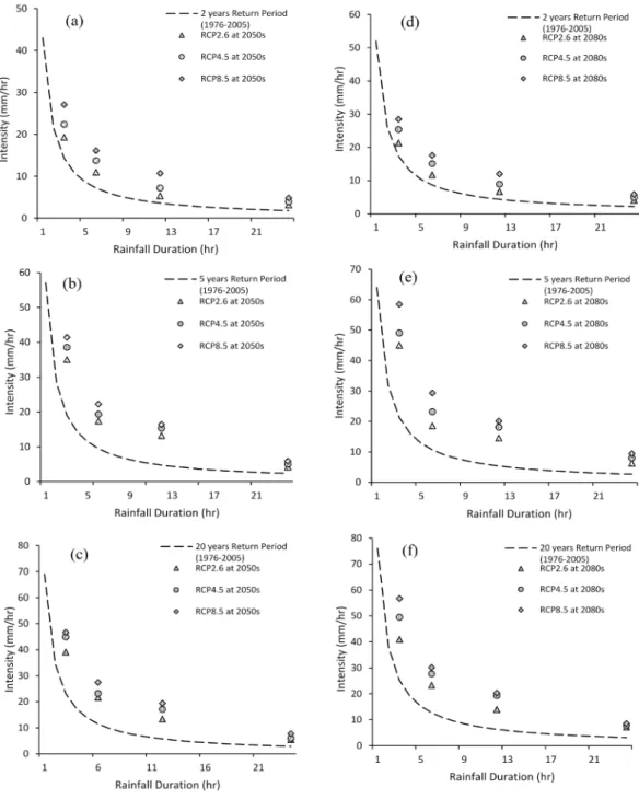
The downscale and disaggregated outputs of the 20 GCMs under RCP2.5, RCP4.5, and RCP8.5 emission scenarios were used to build IDFs for future with durations ranging from 1 to 24 h and return periods of 2, 5, and 20 years. The return periods of 2, 5, and 20 years are chosen which are of practical significance to the design and operation of drainage and irrigation systems. The comparisons between current and future IDF curves under various emission scenarios are shown in Figure 7. It shows that, future scenarios showed higher values for 2-, 5-, and 20 years return periods in Figure 7(a),

for annual maximum rainfall at 12 and 24 h durations, while Gumbel distribution fits better than Gamma at 3 and 6 h duration. Ultimately, GEV seemed to fit better than any other distribution, so we found the distribution of GEV to produce better present and future IDFs. Table 4 also presents a comparison of rainfall intensities at 2-, 5- and 20-year return intervals as annual maximum rainfall is separated into different distributions.

TABLE 4. GEV, Gamma, and Gumbel distributions for annual maximum precipitation (1976-2005) and corresponding intensities for various return periods

Duration

Distribution Parameters

Chi-squared test Intensity (mm/h) at return periods

2 years 5 years 20 years

3 h GEV k = 0.03421, µ=17.32, σ = _66.34 1.325 0.851 19.32 35.07 39.12 Gamma α = 17.32, β = 7.011, γ = 0 1.044 0.772 24.11 33.71 38.77 Gumbel α = 17.423, µ = 72.112 1.015 0.791 27.33 34.17 37.69 Standard deviation 0.51 0.31 0.47 6 h GEV k = 0.13421, µ=19.02, σ = 71.46 0.255 0.912 17.97 17.44 31.66 Gamma α = 11.25, β = 14.61, γ = 0 2.179 0.563 18.39 17.53 28.53 Gumbel α = 22.434, µ = 84.514 1.173 0.741 18.62 17.34 26.39 Standard deviation 0.42 0.46 0.64 12 h GEV k = 0.2421, µ= 21.71, σ = 81.94 0.734 0.853 11.34 13.27 18.41 Gamma α = 9.82, β = 18.43, γ = 0 1.553 0.783 10.56 12.88 16.93 Gumbel α = 37.213, µ = 89.432 1.269 0.733 8.39 11.09 15.38 Standard deviation 0.26 0.41 0.60 24 h GEV k = 0.3021, µ=23.12, σ = 86.57 0.117 0.931 6.17 6.27 9.44 Gamma α = 8.12, β = 22.83, γ = 0 0.994 0.755 5.23 5.59 8.34 Gumbel α = 41.503, µ = 92.731 0.852 0.544 5.39 6.41 7.78 Standard deviation 0.21 0.39 0.61

7(b), 7(c). Similarly, the IDFs curve under all emission scenarios have higher magnitudes at lower rainfall durations. However, the relative differences between the curves reduced with increase of rainfall durations. Similar characteristics was found in in the IDF curves established while developing for future curves under various return periods in Thailand (Shrestha et al. 2017). Moreover, the ensemble GCMs projected non-linear IDFs curves especially at lower return periods for all the RCPs emission scenarios. The rainfall intensities increase with both return periods and emission scenarios, except in 20

years return period of 2050s (Figure 7(c)). This could be attributed to the uncertainties associated with climate models and downscaling techniques adopted. The selected future scenarios RCP2.6, RCP4.5 and RCP8.5 represent low to high greenhouse gas emission scenarios,

and RCP8.5 is broadly a scenario where no strict action is taken. The maximum potential rainfall increments were projected in 2080s under the RCP8.5 emission scenario. The implementation of rigorous disaggregation and analysis techniques in the sense of a newer future climate scenario will further strengthen this strategy.

FIGURE 7. Results of Current and Future IDFs generated from 20 ensemble GCMs for 2-, 5- and 20-years return periods: RCP scenarios (a, b, c, d, e, f) for future

Furthermore, IDFs projection in 2080s under scenarios showed notable change from the baseline condition as in Figure 7(d), 7(e), 7(f)). The weighted ensemble climate models (GCMs) has improved the accuracy of climate projection in this study, since individual GCM produced different future rainfall series. This has been recommended by recent studies because minimize the degree of uncertainty in climate projection (Araji et al. 2018). Overall findings show an increase in potential rainfall for the Cameron Highlands region. Most rainfall stations worldwide lack long-term, higher-temporal rainfall resolution data for lengthy periods, while most GCM outputs are available on a daily time scale. Where the availability of such data is a problem, the Temporary Disaggregation Approach may provide quantified evidence of the impact of climate change on precipitation intensity. One of the main advantages of using temporal disaggregation is its ability to support urban hydrological studies and its practical applications, using only short-term higher-resolution data along with fairly rougher long-term resolution data available in most cities. Short-term sub-daily rainfall at a specific station or nearby stations is needed to generate BLRP parameters using Hyetos. Nevertheless, the BLRP parameters may vary depending on the location and quality of the rainfall data.

CONCLUSION

This study presents an approach based on statistical downscaling of twenty General Circulation Models (GCMs) to develop future IDFs using weighted ensemble means and a rainfall disaggregation tool Hyetos. The results obtained indicate that the method can produce promising results which can be extended to other catchments. Multiplicative change factor downscaling yielded reasonable results in estimating extreme climate variables (i.e. precipitation series) and the downscaled-disaggregated IDFs showed underestimation in rainfall intensity, especially for short durations, hence, it indicates the necessity to correct bias in IDF generation. The generated curves for future scenarios were increased relative to the current situation for all the return periods considered. It has been indicated in this study that, multi model ensemble approach of climate study is providing more reliable projection of climate variables and thus, should be adopted. Furthermore, the statistical approaches for selection of best fitting distributions were Generalized Extreme Value (GEV), Gamma, and Gumbel distributions. Thus, Chi-squared (χ2) test showed the GEV distribution fits better than both Gamma and Gumbel for all the annual maximum rainfall durations and therefore, applied for IDF curves projections. It shows that, IDF curves produced for 2080s periods are higher than both 2050s and baselines periods under 2-, 5-, 20 years return periods. The future studies in this direction

will focus on improving temporal disaggregation methods and achieving more reliable performance of future climate downscaling models in higher resolutions.

ACKNOWLEDGEMENTS

The authors would like to acknowledge the Ministry of Higher Education (MOHE) and Universiti Putra Malaysia (UPM) for sponsoring this research under research number LRGS-NANOMITE/5526305. Authors declare no conflict of interest.

REFERENCES

Abdullah, A.F., Aimrun, W., Nasidi, N.M., Hazari, K., Mohd Sidek, L. & Selamat, Z. 2019. Modelling erosion and

landslides induced by faming activities at hilly areas,

Cameron Highlands, Malaysia. Jurnal Teknologi 81(6): 195-204.

Amanambu, A.C., Li, L., Egbinola, C.N., Obarein, O.A., Mupenzi, C. & Chen, D. 2019. Spatio-temporal variation in rainfall-runoff erosivity due to climate change in the lower Niger Basin, West Africa. CATENA 172: 324-334.

Anandhi, A., Frei, A., Pierson, D.C., Schneiderman, E.M., Zion, M.S., Lounsbury, D. & Matonse, A.H. 2011. Examination

of change factor methodologies for climate change impact

assessment. Water Resources Research 47(3): 1-10. Araji, H.A., Wayayok, A., Bavani, A.M., Amiri, E., Abdullah,

A.F., Daneshian, J. & Teh, C.B.S. 2018. Impacts of climate change on soybean production under different treatments of field experiments considering the uncertainty of general circulation models. Agricultural Water Management 205(2018): 63-71.

Choi, J., Lee, O., Jang, J., Jang, S. & Kim, S. 2019. Future

intensity-depth-frequency curves estimation in korea under representative concentration pathway scenarios of

Fifth assessment report using scale-invariance method. International Journal of Climatology 39(2): 887-900. Chow, V.T., Maidment, D.R. & Mays, L.W. 1988. Applied

hydrology. In McGraw-Hill Series in Water Resources and Environmental Engineering. New York: McGraw-Hill Book

Company.

D-iya, S.G., Gasim, M.B., Toriman, M.E. & Abdullahi, M.G. 2014. Floods in Malaysia: Historical reviews, causes, effects and mtigations approach. International Journal of Interdisciplinary Research and Innovations 2(4): 59-65. Ehmele, F. & Kunz, M. 2019. Flood-related extreme precipitation

in southwestern Germany: Development of a

two-dimensional stochastic precipitation model. Hydrology and Earth System Sciences 23(2): 1083-1102.

Gasim, M.B., Mokhtar, M., Surif, S., Toriman, M.E., Abd. Rahim, S. & Lun, P.I. 2012. Analysis of thirty years recurrent floods of the Pahang River, Malaysia. Asian Journal of Earth Sciences 5(1): 25-35.

Gericke, A., Kiesel, J., Deumlich, D. & Venohr, M. 2019. Recent

and future changes in rainfall erosivity and implications for the soil erosion risk in Brandenburg, NE Germany. Water 11(5): 1-18.

Hanaish, I.S., Ibrahim, K. & Jemain, A.A. 2011. Daily rainfall

disaggregation using HYETOS model for Peninsular

Mathematics, Simulation and Modelling. Wisconsin: World

Scientific and Engineering Academy and Society (WSEAS). pp. 46-50.

Hosking, J.R.M. 1990. L-Moments: Analysis and estimation

of distributions using linear combinations of order

statistics. Journal of Royal Statistical Society. Series B (Methodological) 52(1): 105-124.

Hosking, J.R.M. & Wallis, J.R. 1997. Regional Frequency Analysis: An Approach Based on L-Moments. Cambridge: Cambridge University Press.

IPCC. 2013. Climate Change 2013: The Physical Science Basis. Contribution of Working Group I to the Fifth Assessment Report of the Intergovernmental Panel on Climate Change, edited by Stocker, T.F., Qin, D., Plattner, G.K., Tignor, M.M.B., Allen, S.K., Boschung, J., Nauels, A., Xia, Y., Bex, V. & Midgley, P.M. Cambridge: Cambridge University Press. IPCC. 2014. Climate Change 2014: Synthesis Report.

Contribution of Working Groups I, II and III to the Fifth Assessment Report of the Intergovernmental Panel on Climate Change. Geneva: The Intergovernmental Panel on

Climate Change.

Koutsoyiannis, D. & Onof, C. 2001. Rainfall disaggregation using adjusting procedures on a Poisson cluster model. Journal of Hydrology 246(1-4): 109-122.

Kristvik, E., Johannessen, B.G. & Muthanna, T. 2019. Temporal

downscaling of IDF curves applied to future performance

of local stormwater measures. Sustainability 11(5): 1-24. Liew, S.C., Raghavan, S.V. & Liong, S.Y. 2014. How to construct

future IDF curves, under changing climate, for sites with scarce rainfall records? Hydrological Processes 28(8): 3276-3287.

Mandal, S., Breach, P.A. & Simonovic, S.P. 2016. Uncertainty in

precipitation projection under changing climate conditions:

A regional case study. American Journal of Climate Change 5(1): 116-132.

Mondal, A., Khare, D., Kundu, S., Mukherjee, S., Mukhopadhyay, A. & Mondal, S. 2017. Uncertainty of soil erosion

modelling using open source high resolution and aggregated

DEMs. Geoscience Frontiers 8(3): 425-436.

Nkunzimana, A., Bi, S., Jiang, T., Wu, W. & Abro, M.I. 2019.

Spatiotemporal variation of rainfall and occurrence of

extreme events over burundi during 1960 to 2010. Arabian Journal of Geosciences 12(176): 1-22.

Perkins, S.E., Alexander, L.V. & Nairn, J.R. 2012. Increasing

frequency, intensity and duration of observed global

heatwaves and warm spells. Geophysical Research Letters 39(20): 1-5.

Razali, A., Syed Ismail, S.N., Awang, S., Praveena, S.M. & Zainal Abidin, E. 2018. Land use change in highland area and its

impact on river water quality: A review of case studies in

Malaysia. Ecological Processes 7(19): 1-17.

Sardari, M.R.A., Bazrafshan, O., Panagopoulos, T. & Sardooi, E.R. 2019. Modeling the impact of climate change and land

use change scenarios on soil erosion at the Minab Dam

watershed. Sustainability 11(2): 1-21.

Shrestha, D.P. & Jetten, V.G. 2018. Modelling erosion on a daily

basis, an adaptation of the MMF approach. International Journal of Applied Earth Observation and Geoinformation 64: 117-131.

Shrestha, A., Babel, M.S., Weesakul, S. & Vojinovic, Z. 2017.

Developing Intensity-Duration-Frequency (IDF) curves under climate change uncertainty: The case of Bangkok,

Thailand. Water 9(2): 1-22.

Singh, G. & Rabindra, K.P. 2017. Grid-cell based assessment of soil erosion potential for identification of critical erosion

prone areas using USLE, GIS and remote sensing: A case

study in the Kapgari watershed, India. International Soil and Water Conservation Research 5(3): 202-211.

Song, X., Zhang, J., Zou, X., Zhang, C., AghaKouchak, A. & Kong, F. 2019. Changes in precipitation extremes in the beijing metropolitan area during 1960-2012. Atmospheric Research 222(1): 134-153.

Zhiying, L. & Fang, H. 2016. Impacts of climate change on water erosion: A Review. Earth-Science Reviews 163: 94-117.

Nuraddeen Mukhtar Nasidi*, Aimrun Wayayok, Ahmad Fikri

Abdullah & Muhamad Saufi Mohd Kassim

Department of Biological and Agricultural Engineering Faculty of Engineering

Universiti Putra Malaysia

43300 UPM Serdang, Selangor Darul Ehsan Malaysia

Aimrun Wayayok, Ahmad Fikri Abdullah & Muhamad Saufi

Mohd Kassim

SMART Farming Technology Research Center Faculty of Engineering

Universiti Putra Malaysia

43300 UPM Serdang, Selangor Darul Ehsan Malaysia

Nuraddeen Mukhtar Nasidi*

Department of Agricultural and Environmental Engineering Bayero University

Kano, P.M.B. 3011

Gwarzo Road Kano - Nigeria

*Corresponding author; email: [email protected]

Received: 10 March 2020 Accepted: 9 May 2020