Masters Theses Student Research & Creative Works
Spring 2014
Two driven pile load tests for use in Missouri LRFD
guidelines
Matthew Garry Stuckmeyer
Follow this and additional works at:http://scholarsmine.mst.edu/masters_theses Part of theCivil Engineering Commons
Department: Civil, Architectural and Environmental Engineering
This Thesis - Open Access is brought to you for free and open access by the Student Research & Creative Works at Scholars' Mine. It has been accepted for inclusion in Masters Theses by an authorized administrator of Scholars' Mine. For more information, please [email protected].
Recommended Citation
TWO DRIVEN PILE LOAD TESTS FOR USE IN MISSOURI LRFD GUIDELINES by
MATTHEW GARRY STUCKMEYER A THESIS
Presented to the Faculty of the Graduate School of the MISSOURI UNIVERSITY OF SCIENCE AND TECHNOLOGY
In Partial Fulfillment of the Requirements for the Degree MASTER OF SCIENCE IN CIVIL ENGINEERING
2014 Approved by
Dr. Ronaldo Luna, Advisor Dr. J. David Rogers
ABSTRACT
A static pile load test program was initiated by the Missouri Department of Transportation (MoDOT) to evaluate the use of pile load tests in Missouri LRFD guidelines. The program’s approach involves two phases to achieve the appropriate levels of reliability for driven piles in the state of Missouri. This thesis focuses on the data collection efforts of Phase 1. Two quick static pile load tests were performed to failure on test piles in the Southeast Lowlands geologic region of Missouri. The piles were dynamically monitored during installation and subsequent restrike tests performed. The results of the static and dynamic pile testing were evaluated and interpreted. Overall, the nominal resistances predicted by dynamic tests (CAPWAP) at beginning of restrike (BOR) compared well to the results of the static load tests evaluated using Davisson’s method (at these specific sites). A comparison of the load transfer distributions from the dynamic and static load tests provided mixed results. The effects of pile set-up after driving are a significant factor to consider in determining the need for a restrike. The additional resistance available following pile setup can have a substantial effect on the nominal resistance determined using dynamic methods. When BOR capacities are measured using dynamic methods they can be used with confidence for the calibration of resistance factors with respective pile types and geologic units. Available pile load test data sets from Missouri’s neighboring states and previous efforts conducted in Missouri were compiled as well. Two recently available pile load test databases were evaluated and considered for the upcoming phase to conduct calibration of resistance factors.
ACKNOWLEDGMENTS
I would like to express my sincere appreciation and gratitude to my advisor, Dr. Ronaldo Luna, for his support, motivation, and guidance throughout this research program. The direction and collaboration provided by Dr. Luna has made my time in graduate school a very memorable learning experience. I would also like to thank my committee members Dr. J. David Rogers and Craig Kaibel; their comments, suggestions, and additional motivation was very valuable. I would also like to thank fellow Missouri S&T graduate student Kerry Magner for his continuous input and assistance. Thank you to several staff members of the Missouri S&T Civil Engineering Department including, Brian Swift, Gary Abbott, and John Bullock for their help with high-bay activities and field work.
Additionally, I would like to thank the Missouri Department of Transportation (MoDOT) for being the primary financial supporter of this research effort. Thank you to all the MoDOT personnel, both in Jefferson City and the multiple District offices, for their contribution and cooperation throughout the process. Special thanks to Thomas Fennessey and Jen Harper, MoDOT personnel, for their continued communication and support. The author would also like to thank Craig Kaibel and Joe Cravens of Geotechnology, Inc. for conducting the dynamic testing and associated data reduction portions of this research. Their knowledge and input was very valuable to the success of this project.
I am extremely grateful to my parents, Garry and Dianne, sister, Katie, and fiancée, Ashley for their consistent love and encouragement. The successful completion of this thesis would not have been possible without the continuous support of my family and friends.
TABLE OF CONTENTS
Page
ABSTRACT ... iii
ACKNOWLEDGMENTS ... iv
LIST OF ILLUSTRATIONS ... x
LIST OF TABLES ... xii
SECTION 1. INTRODUCTION ... 1
1.1. INTRODUCTION ... 1
1.2. PILE DESIGN IN MISSOURI ... 2
1.3. RESEARCH OBJECTIVES ... 3
1.4. THESIS ORGANIZATION ... 4
2. LITERATURE REVIEW ... 6
2.1. INTRODUCTION ... 6
2.2. DRIVEN PILE FOUNDATIONS ... 6
2.2.1. Timber Piles ... 7 2.2.2. Steel Piles ... 7 Pipe piles ...8 2.2.2.1 H-piles ...8 2.2.2.2 2.2.3. Concrete Piles ... 8
2.3. DETERMINING PILE RESISTANCE ... 9
2.3.1. Static Methods. ... 10
2.3.2. Wave Equation Analysis ... 11
2.3.3. High-Strain Dynamic Testing ... 11
PDA...12
2.3.3.1 Wave equation/Case method analysis remarks ...12
2.3.3.2 CAPWAP ...13
2.3.3.3 2.3.4. Static Pile Load Tests ... 13
Loading procedures ...13
2.3.4.1 2.3.4.1.1 Slow Maintained Load (ML) method ... 13
Interpretation of test results ...14
2.3.4.2 2.3.4.2.1 Davisson (1972) method ... 15
2.3.4.2.2 Chin (1970) method ... 15
2.3.4.2.3 De Beer (1967) method ... 16
2.3.4.2.4 Brinch Hansen (1963) 90 Percent Criterion ... 16
2.3.4.2.5 Mazurkiewicz (1972) method ... 16
2.4. PILE DESIGN METHODS ... 17
2.4.1. Allowable Stress Design (ASD) ... 18
2.4.2. Load and Resistance Factor Design (LRFD) ... 19
2.5. VARIOUS STATES LRFD IMPLENTATION EFFORTS ... 21
2.5.1. Florida ... 22
2.5.2. Illinois ... 23
2.5.3. Louisiana ... 24
2.5.4. Wisconsin ... 24
2.5.5. Iowa... 25
2.6. MISSOURI LRFD IMPLEMENTATION EFFORTS ... 26
2.6.1. Former Research Projects ... 26
2.6.2. Current Research Project ... 29
3. MISSOURI’S STATE OF PRACTICE ... 31
3.1. BACKGROUND ... 31
3.2. MODOT’s STATE OF PRACTICE ... 31
3.2.1. Pile Types... 33
3.2.2. Static Methods ... 33
3.2.3. Pile Structural Resistance Factors ... 33
3.2.4. Geotechnical Resistance Factors ... 34
3.2.5. Special Provisions ... 34
Dynamic testing ...35
3.2.5.1 Static Pile Load Test (PLT) ...36
3.2.5.2 3.3. GEOLOGY IN MISSOURI ... 37
3.3.1. The Ozark Highlands ... 37
3.3.3. The Glaciated Plains ... 38
3.3.4. The Southeast Lowlands ... 39
4. PILE LOAD TEST PROGRAM METHODS ... 40
4.1. INTRODUCTION ... 40
4.2. TEST EQUIPMENT ... 40
4.2.1. Load Frame Design. ... 40
4.2.2. Load Frame Construction ... 41
4.2.3. Load Application and Measurement ... 41
4.3. SUPPORTING INSTRUMENTATION ... 42
4.3.1. Applied Load ... 42
4.3.2. Pile Head Displacement ... 43
4.3.3. Incremental Strain ... 44 Concrete embeddable VWSGs ...44 4.3.3.1 Weldable VWSGs ...45 4.3.3.2 4.3.4. Redundant Instrumentation ... 45
4.4. DATA ACQUISITION SYSTEM ... 46
4.4.1. System Requirements ... 46
4.4.2. Description of the Completed System ... 46
4.5. DYNAMIC MONITORING PROCEDURE ... 50
4.6. STATIC PILE LOAD TEST PROCEDURE ... 51
4.7. DATA REDUCTION ... 52
5. RESULTS OF PILE LOAD TESTS ... 55
5.1. TESTING SITES ... 55
5.2. SIKESTON, MISSOURI ... 56
5.2.1. Site and Project Description... 56
5.2.2. Subsurface Conditions ... 58
Geology ...58
5.2.2.1 Soil and groundwater ...58
5.2.2.2 5.2.3. Static and Wave Equation Analyses and Results ... 59
Static analysis...59
5.2.3.1 Wave equation analysis...60 5.2.3.2
5.2.4. Anchor Pile & Test Pile Installation ... 61
5.2.5. Dynamic Testing ... 62
5.2.6. Dynamic Testing Results ... 62
5.2.7. Test Pile Instrumentation. ... 63
5.2.8. Static Load Test ... 67
5.2.9. Static Load Test Results... 67
5.2.9.1.1 Nominal resistance ... 69
5.2.9.1.2 Load transfer distribution ... 73
5.3. POPLAR BLUFF, MISSOURI ... 74
5.3.1. Site and Project Description... 75
5.3.2. Subsurface Conditions ... 75
Geology ...76
5.3.2.1 Soil and groundwater ...76
5.3.2.2 5.3.3. Static and Wave Equation Analyses and Results ... 77
Static analysis...77
5.3.3.1 Wave equation analysis ...78
5.3.3.2 5.3.4. Anchor Pile & Test Pile Installation ... 79
5.3.5. Dynamic Testing ... 80
5.3.6. Dynamic Testing Results ... 80
5.3.7. Test Pile Instrumentation Installatio ... 81
5.3.8. Static Load Test ... 83
5.3.9. Static load test results ... 84
5.3.9.1.1 Nominal resistance ... 86
5.3.9.1.2 Load transfer distribution ... 90
6. SUMMARY AND DISCUSSION OF PILE LOAD TEST RESULTS ... 91
6.1. INTRODUCTION ... 91
6.2. PILE LOAD TEST – DYNAMIC AND STATIC ... 91
6.2.1. Dynamic Load Tests ... 91
6.2.2. Static Load Test – Nominal Resistance ... 93
6.2.3. Static Load Test – Load Transfer Distribution ... 94
7. COMPILATION OF PILE LOAD TEST DATA ... 99 7.1. INTRODUCTION ... 99 7.2. PLT DATABASE CONSIDERATIONS ... 99 7.2.1. Comprehensive Data ... 99 General ...100 7.2.1.1 Design ...102 7.2.1.2 Testing...103 7.2.1.3 7.2.2. Data Quality ... 103 7.2.3. Database Queries ... 104
7.3. AVAILABLE DATA SETS ... 105
7.3.1. FHWA Deep Foundations Load Test Database ... 105
Installation...106
7.3.1.1 Overview ...106
7.3.1.2 7.3.2. Iowa State’s PILOT Database ... 109
Installation...109
7.3.2.1 Overview ...109
7.3.2.2 7.3.3. Missouri Previous Efforts ... 111
7.3.4. Current Research Project ... 112
8. CONCLUSIONS AND RECOMMENDATIONS ... 113
8.1. CONCLUSIONS ... 113
8.2. RECOMMENDATIONS ... 114
APPENDICES A. MODOT BRIDGE PLANS AND SPECIAL PROVISIONS ON CD-ROM 116 B. STATIC ANALYSIS RESULTS ON CD-ROM ... 118
C. WEAP ANALYSES AND DYNAMIC TESTING REPORTS ON CD-ROM ... 120
D. STATIC LOAD TEST DATA AND RESULTS ON CD-ROM ... 122
E. PILE LOAD TEST DATA FROM OTHER RESEARCH PROJECTS ON CD-ROM ... 124
BIBLIOGRAPHY ... 126
LIST OF ILLUSTRATIONS
Figure Page
2.1 Extent of LRFD Implementation Following Oct. 1, 2007 Deadline ... 22
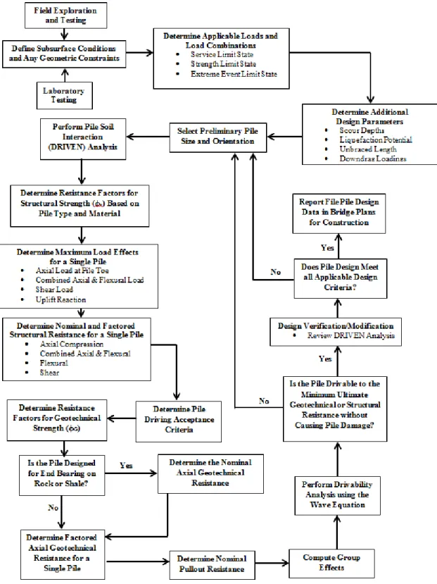
3.1 Interpreted Flow Chart of MoDOT Pile Design Process ... 32
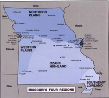
3.2 Missouri’s Geologic Regions ... 37
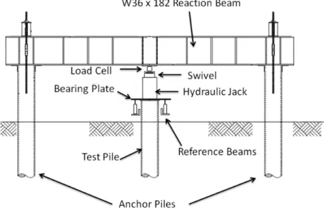
4.1 Diagram of the Pile Load Test Components ... 42
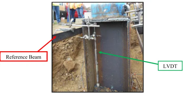
4.2 Orientation of LVDT When Mounted to the Reference Beam ... 43
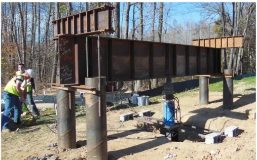
4.3 Orientation of Reference Beams With Respect to Load Frame ... 44
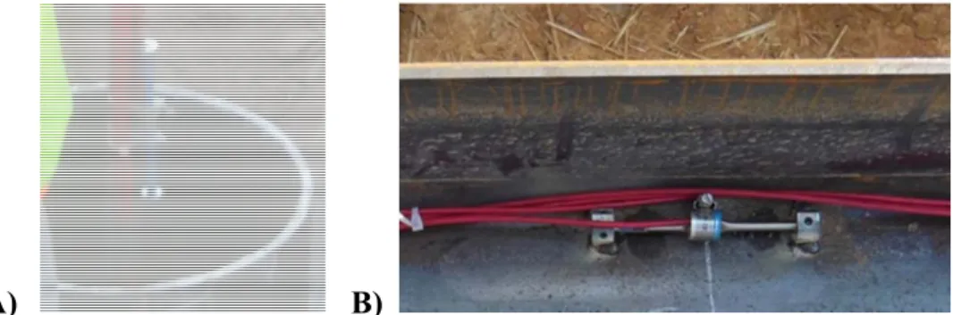
4.4 The VWSGs Used to Measure Load Transfer Distribution.. ... 45
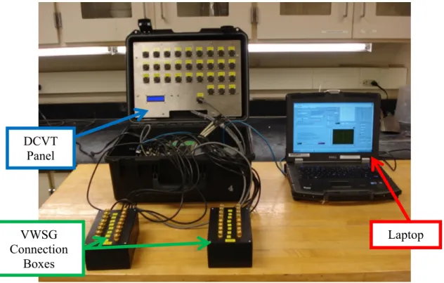
4.5 Data Acquisition System Peripherals... 50
5.1 Static Pile Load Testing Locations ... 55
5.2 A7956 Site Location Map ... 56
5.3 MoDOT Illustration of the Proposed Structure ... 57
5.4 A7956 Soil Profile along the Test Pile ... 59
5.5 A7956 Reaction Pile Installation ... 61
5.6 A7956 CAPWAP Wave Match and Load-Displacement Curve ... 63
5.7 Installation of the Center Bar and VWSGs ... 64
5.8 Process of Test Pile Concrete Placement. ... 65
5.9 Completed A7956 Pile Load Test Set-up ... 67
5.10 A7956 Static Load Test Results ... 69
5.11 Interpretation of A7956 Nom. Resistance Using the Davisson (1972) Method ... 70
5.12 Interpretation of A7956 Nom. Resistance Using the Chin (1970) Method ... 70
5.13 Interpretation of A7956 Nom. Resistance Using the De Beer (1968) Method ... 71
5.14 Interpretation of A7956 Nom. Resistance Using the Mazerkiewicz (1980) Method ... 71
5.15 Interpretation of A7956 Nom. Resistance Using the Brinch Hansen 90% (1963) Method ... 72
5.16 A7956 Load Transfer Plot ... 74
5.17 A7669 Site Location Map ... 74
5.18 MoDOT Illustration of A7669 Proposed Structure ... 75
5.20 A7669 Test Pile Installation ... 79
5.21 A7669 CAPWAP Wave Match and Load-Displacement Curve ... 81
5.22 H-Pile Instrumentation Process... 82
5.23 Completed A7669 Pile Load Test Set-up ... 83
5.24 A7669 Static Load Test Results ... 85
5.25 Interpretation of A7669 Nom. Resistance Using the Davisson (1972) Method ... 86
5.26 Interpretation of A7669 Nom. Resistance Using the Chin (1970) Method ... 87
5.27 Interpretation of A7669 Nom. Resistance Using the De Beer (1968) Method ... 87
5.28 Interpretation of A7669 Nom. Resistance Using the Mazurkiewicz (1980) Method ... 88
5.29 Interpretation of A7669 Nom. Resistance Using the Brinch Hansen 90% (1963) Method ... 88
5.30 A7669 Load Transfer Plot ... 90
7.1 Data Requirements of a PLT Record ... 100
7.2 Example General Data Requirements of a PLT ... 101
7.3 Example Design Data Requirements of a PLT ... 102
7.4 Example Test Data Requirements of a PLT Record ... 104
7.5 DFLTD User Query Window ... 107
7.6 PILOT's Display Form ... 109
LIST OF TABLES
Table Page
2.1 Factor of Safety Based on Level of Construction Control (AASHTO, 2004) ... 19
2.2 Suggested Geotechnical Resistance Factors (adapted from Kebede, 2010) ... 28
2.3 Results of Neighboring State Questionnaires……….30
3.1 MoDOT Pile Structural Resistance Factors ... 34
3.2 MoDOT Geotechnical Resistance Factors ... 34
3.3 MoDOT Approved Manufacturers and Products for Dynamic Pile Testing ... 35
3.4 Minimum Restrike Durations Based on Subsurface Materials ... 36
4.1 Data Acquisition Components ... 48
4.2 Instrument Connection Locations Within the DAS ... 51
4.3 Geokon VWSG Calibration Factors ... 53
5.1 A7956 Foundation Data (adapted from MoDOT Plans, 2013) ... 58
5.2 A7956 WEAP Analysis Results for Gain/Loss Ratios ... 60
5.3 Summary of CAPWAP Estimated Nominal Resistance for the A7956 test pile ... 62
5.4 A7956 Load Test Schedule ... 68
5.5 Parameters Used in A7956 Data Reduction ... 68
5.6 Summary of Interpreted A7956 Nominal Resistances ... 72
5.7 Comparison of A7956 Nominal Resistance Results ... 73
5.8 A7669 Foundation Data ... 76
5.9 A7669 WEAP Analysis Results for Gain/Loss Ratios ... 78
5.10 Nominal Resistances Estimated From the A7669 CAPWAP Analysis ... 80
5.11 A7669 Loading Schedule ... 84
5.12 Parameters Used in the A7669 Data Reduction ... 85
5.13 Summary of Interpreted A7669 Nominal Resistance ... 89
5.14 Comparison of A7669 Pile Nominal Resistance Results ... 89
6.1 Nominal Resistance Estimated From the CAPWAP Analyses ... 91
6.2 Summary of Static and Dynamic Load Test Results ... 94
6.3 Load Transfer Distribution Results ... 95
7.1 Distribution of DFLTD PLT records from Missouri and Missouri’s Neighboring States ... 108
1.INTRODUCTION
1.1.INTRODUCTION
Driven piles are the most common foundation system used in nearly 10,000 bridges encompassed within Missouri’s state highway system. The geotechnical community in the United States has traditionally used the Allowable Stress Design (ASD) method to produce sufficient structural foundations (DiMaggio et al. 1999). ASD compares the actual forces estimated to be applied to the structure to the structure’s available resistance, or strength, through a value known as the factor of safety (FS). The FS is a summary of the engineer’s best estimate of the uncertainty associated with the project as a whole. Using the FS to determine the design loads of a foundation often reflect conservative estimates of a member’s actual available resistances. Traditionally, different magnitudes of FS have been used to reflect the different levels of control in foundation design and construction, as well as past experience and engineering judgment (Paikowsky, 2004). However, it has long been recognized that standard bridge design specifications based on ASD do not promote a consistent reliability for design (AbdelSalam, 2010). Realizing this deficiency, extensive research efforts have been devoted to the development of a more rational design approach known as Load and Resistance Factor Design (LRFD). LRFD has been well established in design codes around the world for Structural Engineering, and was first adopted in North America through the American Concrete Institute (ACI) Code in 1953 (DiMaggio et al. 1999). The objective of LRFD is to produce engineering designs with consistent levels of reliability using procedures from probability theory to ensure a prescribed margin of safety (Paikowsky, 2004). Under LRFD, the uncertainties in loading are assessed separately from the uncertainties in resistance through load factors and resistance factors, respectively. The load factors and resistance factor are applied in such a way that the engineer is essentially over-estimating the loads on the structure and underestimating the structure’s strength, thus assuring a consistent level of safety.
In 1994, the American Association of State Highway and Transportation Officials (AASHTO) published the first edition of LRFD bridge specifications. The
new LRFD specification contains comprehensive design and construction guidance on both structural and geotechnical features. Initial use of the new specification, however, showed that the approach used in LRFD for structures is not fully compatible with geotechnical design needs (DiMaggio et al. 1999). As a result many geotechnical engineers reverted back to the ASD method of designing foundations that they were accustomed to using in the past. The structural engineers using the LRFD method to design the bridge’s superstructure and the geotechnical engineers designing the substructure using ASD not only created uneconomical designs but also decreased the reliability of the designs.
In order to produce more reliable, consistent designs AASHTO and the Federal Highway Administration (FHWA) issued a policy memorandum on June 28, 2000, requiring all new bridges initiated after October 1, 2007, to be designed using the LRFD approach (Densmore, 2000). AASHTO included resistance factors in the LRFD specifications developed from a collection of Static Pile Load Test (PLT) data from around the U.S. However, these national resistance factors were overly conservative when applied to localized regions because of the variability in the geology and construction practices used to calibrate them. For this reason, AASHTO permitted state Departments of Transportation (DOTs) to develop their own resistance factors based on regional practices and geology to minimize the unnecessary conservatism built into a design. Following the authorization of regional resistance factors, many states such as Florida, Illinois, Washington, and Iowa have all published studies recommending LRFD resistance factors for driven pile foundations within their respective states.
1.2.PILE DESIGN IN MISSOURI
Upon the inception of LRFD in Missouri, the Missouri Department of Transportation (MoDOT) adopted the resistance factors from the AASHTO LRFD Bridge Design Specifications (2010) for designing bridge pile foundations. However, due to the relatively low resistance factors associated with the analysis methods commonly employed by MoDOT, the acquired design loads continue to reflect conservative estimates of a member’s available resistance. As a result, MoDOT is unable to gain from the advantages encompassed in LRFD design.
In 2008, MoDOT supported its first research program to develop a series of LRFD specifications based on the local geotechnical practices and geology within the state. Upon the project’s completion in 2010, a newly developed set of resistance factors were calibrated using existing data from historical construction records of dynamic testing of piles. That is, Pile Driving Analyzer (PDA) and CAse Pile Wave Analysis Program (CAPWAP) software. Although the results of the program suggested the current resistance factors used should be increased, no records of static pile load test data were available to evaluate the actual ultimate capacity of the piles. Therefore, the newly calibrated resistance factors were developed under the strict assumption that dynamic testing methods provide the actual ultimate capacity values.
To validate this assumption a subsequent research project entitled, Evaluation of Pile Load Test for Use in Missouri LRFD Guidelines, was initiated. This thesis will discuss the current research efforts to evaluate the previously calibrated resistance factors based on high-strain dynamic testing methods for use in Missouri.
1.3.RESEARCH OBJECTIVES
The research provided herein is dedicated to allow MoDOT to produce more reliable and economically efficient design for pile foundations by accomplishing the following objectives:
Evaluate MoDOT’s current practice for pile foundations and provide recommendations for improvement in future practice, as well as for future research.
Develop research grade, static pile load test data sets from previously characterized locations within the Missouri highway system.
Evaluate the ability of high-strain dynamic testing to predict the actual nominal resistance measured by the static pile load tests, in hope of proving the accuracy of the 2008-10 developed resistance factors
Compile the data collected from Missouri and it’s neighboring states to assist in the establishment of a database and regional resistance factor calibration in a future phase.
Propose recommendations to improve pile load testing procedures for future development of LRFD resistance factors in future research programs.
1.4.THESIS ORGANIZATION
The research provided herein consists of a literature review of driven piles summarizing: various methods for determining pile resistance, two methods used to design piles, and various states, including Missouri, efforts to accommodate LRFD design. MoDOT’s state-of-practice and the multiple geologic regions found in Missouri are discussed followed by the methods, results, and data compilation of the current research effort. The thesis is organized as follows:
Section 1 introduces the research effort.
Section 2 describes piles in general, various methods for determining pile
resistance (static analysis, wave equation analysis, high-strain dynamic testing, and static load testing). Two methods used to design piles (Allowable Stress Design and Load and Resistance Factor Design) are introduced and previous research programs devoted toward the development of regionally calibrated resistance factors are discussed.
Section 3 discusses MoDOT’s effort to implement LRFD, MoDOT’s current
state-of-practice and procedure for designing pile foundations including common types, sizes, and methods for determining resistance and length, together with an overview of Missouri’s geological regions.
Section 4 discusses the methods used throughout the pile load test program,
including descriptions of the test equipment, instrumentation, and data acquisition system used, as well as an outline of the testing procedures and data reduction procedures.
Section 5 discusses the results of two (2) pile load tests conducted at different sites within the Missouri highway system in the Southeast Lowlands of Missouri. Section 6 provides a summary and discussion of the results presented in Section 5.
Section 7 discusses the effort established to compile datasets from projects
completed in Missouri’s neighboring states and previous projects completed in Missouri.
Section 8 provides conclusions based on the research presented herein, as well as recommendations for the future practice for MoDOT and future research projects.
The appendices include MoDOT bridge plans, MoDOT special provisions, static
analysis results, GRL WEAP analysis results, dynamic testing reports (produced by Geotechnology, Inc.), unreduced static pile load data, and static pile load test results associated with each of the load tests performed during Phase I of this research project. A series of files containing pile load test data from other research projects are also included.
2.LITERATURE REVIEW
2.1.INTRODUCTION
Foundations are the structural components that distribute a structure’s load to the soil. Composed of concrete, steel, wood, or a combination thereof, these elements are most commonly characterized as either shallow foundations or deep foundations. Shallow foundations (spread footings, wall footings, and mat foundations) transfer loads to near-surface soils. In contrast, deep foundations (both piles and drilled shafts) transmit some or all of the loads to a depth at which adequate support becomes available (Prakash, 1990). Whenever possible, shallow foundations are used because they are both cost effective and simple to construct. However, when the construction of shallow foundations is not feasible (i.e., when the required loads cannot be adequately supported at shallow depths), deep foundations provide an alternative solution. Based on the objectives of this research, driven piles will be the only foundation type discussed herein. The following sections will provide a brief overview of pile foundations, discuss various methods for determining pile resistance, and introduce two methods used to design piles.
2.2.DRIVEN PILE FOUNDATIONS
Piles are long, slender, prefabricated structural elements that are typically installed by either hammering or driving them into the ground. Pile foundations are generally used when proper bearing stratum are unavailable at shallow depths. They may also be used for structure’s with large structural loads that would make shallow foundations would either uneconomical or infeasible (Das, 2007). Deep foundations provide resistance through mechanisms known as end-bearing and side friction. End-bearing is the resistance contributed by the area of the tip (or toe) of the pile; side friction is the development of resistive forces along the pile’s length due to the friction/adhesion between the soil and pile during driving (Prakash, 1990).
When bedrock is located within a reasonable distance from the ground’s surface, piles are commonly driven until they come into contact with the underlying bedrock. As a result, the pile’s nominal resistance is significantly dependent on the bedrock
material’s load-bearing capacity (Das, 2007). Piles that obtain their resistance in this manner are classified as end-bearing piles. When bedrock is located at great depths and the installation of end-bearing piles is uneconomical, driven piles must rely largely on their side friction for resistance. Naturally, these piles are categorized as friction piles.
Piles are available in a variety of materials, diameters, and lengths, each depending on their application within a project. The following sections will present some of the common types of piles, as well as, each type’s most common size and use.
2.2.1.Timber Piles. Throughout history, timber piles have been the most widely used form of piling. Derived from trunks of trees, timber piles are still a common option for use today due to their low construction cost. Timber piles can be fabricated from a variety of acceptable trees. Both Southern Yellow Pine and West Coast Douglas Fir are most commonly used today because they are tall, straight, and relatively abundant (Coduto, 2001). The dimensions of a timber pile are dependent on the specific tree being used. Diameters between 6 and 18 inches and lengths of up to 60 feet are, however, most typical (Das, 2007). Timber piles can be spliced together, though this process usually increases the cost of construction significantly. If the required length cannot be achieved with a single timber pile, an alternative material is typically chosen. Timber piles can carry design loads of up to 100 kips. They are best suited for light driving conditions, however, because they are more susceptible to damage during driving than piles made of other materials. Timber piles are most commonly used as friction piles in either loose sand or soft to medium clays (Prakash, 1990).
2.2.2.Steel Piles. Steel piles are commonly used in practice for projects with either difficult ground conditions or heavily loaded structures. The high strength and ductility of steel makes them ideal for driving in hard soils. Steel’s high tensile strength also makes steel piles the common choice for tensile loaded applications. Steel piles are often the primary pile choice in areas with variable bedrock depths because they are easy to both splice and cut (Prakash, 1990). Disadvantages of steel piles include cost, noise during installation, and susceptibility to corrosion (Coduto, 2001). The most common steel piles used in engineering practice are pipe piles and H-piles.
Pipe piles. Pipe piles are available in a variety of diameters and wall
2.2.2.1
thicknesses; diameters between 8 and 36 inches and wall thicknesses of up to ½ inch are typical (Coduto, 2001). These long cylinders can be driven open-ended or closed-end by welding a thick plate to the end of the pile. Closed-end pipe piles are commonly used as friction piles due to the increase in resistance created by the closed end. Consequently, the closed end causes a larger displacement of soil to occur making driving more difficult.
In the United States pipe piles are often filled with concrete after driving (Prakash, 1990). Once concrete has been placed in a pipe pile, it is referred to as a cast-in-place (CIP) pile. The placement of concrete provides the advantages of increased uplift resistance due to the additional dead-weight, greater shear and moment resistance due to the concrete’s strength, and a longer service-life in corrosive environments (Coduto, 2001). The design resistance of CIP piles can be as high as 250 kips. However, when lengths surpass 80 feet, the cost of CIP piles generally becomes uneconomical (Prakash, 1990).
H-piles. H-piles are steel members manufactured specifically to be used
2.2.2.2
as piles. Their shape resembles wither wide flange (WF) beams or I-beams. The primary difference is the web and flange thicknesses of H-piles are equal (the web thickness of both WF beams and I-beams is thinner than the flanges) (Prakash, 1990). H-piles are suitable for use in hard driving conditions because they displace a relatively small amount of soil during driving. Thus, H-piles are typically used as end-bearing piles and are driven to bedrock (Coduto, 2001). They may be damaged or deflected from vertical during driving through hard layers or past major obstructions. As a result, hardened steel points are regularly welded to the pile toe to provide protection during driving (Das, 2007).
2.2.3. Concrete Piles. Concrete piles are pre-cast, reinforced concrete members designed to withstand damage from not only handling and driving but also service loads (Prakash, 1990). Concrete piles are typically wither square or orthogonal in shape. Reinforcement is provided within the pile using lateral bars and ties, pre-tension, or post-tension methods. In the past, conventionally reinforced concrete piles (lateral bars and ties) were very common. Today, however, pre-stressed methods (pre-tension or
post-tension) are almost always used in the U.S. (Coduto, 2001). Although concrete piles are more susceptible than steel piles to damage in hard driving conditions, they cost less than steel piles and can be used in corrosive environments (where steel is susceptible to degradation). Concrete piles can be used as either end-bearing or friction piles, although they are more difficult to cut and splice than steel piles. They are best suited for use in either end-bearing when bedrock depths are well defined or as friction piles that will not reach refusal (Coduto, 2001).
2.3.DETERMINING PILE RESISTANCE
An engineer must consider a number of options when designing a foundation with piles. These options include: pile type, length, diameter, shape, number and spacing. While the selection of these qualities is often determined by not only previous experience but also the availability of materials, the end result of all pile designs are the same: they must provide the required load-bearing resistance needed to support the structure. Although the nominal load of a structure is usually well-defined by the structural engineer, determining the actual nominal resistance available from the geotechnical engineer’s design is not as straightforward. The uncertainties in the geotechnical design are primarily attributed to the prediction of the strength-deformation behaviors of soil and the overall performance of the soil-foundation system (Goble, 1996).
The maximum load a pile can carry before failing is known as the pile’s nominal resistance (in LRFD design. It should be noted that piles provide axial, lateral, and pullout (or tension) resistances and although each of these modes can be evaluated separately, axial resistance will be the only form discussed herein. Furthermore, the term “resistance” throughout the remainder of this thesis will be in reference to the nominal resistance in the axial direction. The nominal axial resistance of a pile is a combination of the resistances provided by the end-bearing and the skin friction. The nominal resistance of an axially loaded pile is expressed in the following equation:
(2.1) where Qeb represents the end-bearing resistance and
Qt represents the skin friction resistance.
The following sections will discuss the various methods for determining pile resistance including: static methods, wave equation analysis, high-strain dynamic testing, and low-strain static testing.
2.3.1.Static Methods. Static methods are empirical equations that usemeasured strength parameters from subsurface materials to predict the available side-friction and toe-bearing resistances of a pile during driving. Because in-situ tests are both subjective and highly-variable, the correlations provided by static methods have been viewed as less precise and conservative (Fang et al., 1975). Because geotechnical investigations are performed before construction is initiated, static methods are attractive because the geotechnical data needed for their calculation are usually readily available.
Static methods are most often used to initiate a preliminary design because they are the quickest and cheapest way to predict a pile’s nominal resistance. These methods, however, require an engineer to both recognize and understand their limitations. Unlike shallow foundations, the installation of deep foundations causes changes to the local soil conditions. For example, as piles are driven into the ground, the displaced soil induces large horizontal stresses which consolidate the soil, changing its engineering properties (Coduto, 2001). As a result, the strength parameters measured before installation (in the geotechnical investigation) are not necessarily representative of the soil’s strength parameters after installation.
The Federal Highway Administration (FHWA) provides a compilation of static methods to predict pile resistance through the computer program DRIVEN. This program is commonly used by the Missouri Department of Transportation (MoDOT) to create the preliminary design and follows both the methods and the equations presented by Thurman (1964), Meyerhof (1976), Nordlund (1963, 1979), Tomlinson (1980, 1986), Cheney and Chassie (1982), and Hannigan et al. (1997). The pile’s nominal resistance is determined at selected depth intervals from the soil profile once the entire soil profile is input into the program. At each interval, DRIVEN distinguishes how much of the nominal resistance is contributed by skin-friction and how much is contributed by
end-bearing. DRIVEN also has the ability to analyze multiple water tables, negative skin friction, and scour (Cravens, 2011).
2.3.2.Wave Equation Analysis. The wave equation is a numerical model that simulates the pile driving process by applying the theory of one-dimensional stress wave propagation (Rausche et al., 2012). Smith (1962) used a series of masses, springs, and dashpots to model all of the aspects influencing pile driving, including hammer mass and travel, combustion in a diesel hammer, helmet mass, cushion stiffness, hammer efficiency, soil strength, elastic properties of the pile, and so forth. The wave equation analysis then calculates the velocities, displacements, and resulting forces as a result of the impact per time for all of the elements in the system (Fang et al., 1975).
Many companies have commercially produced computer software to simplify use of the wave equation. The Wave Equation Analysis of Piles (GRLWEAP), produced by Pile Dynamics, Inc. is one of the most commonly used of these programs. When performed before driving, a WEAP analysis can be used to estimate the driving resistance, pile stresses, and hammer performance.
2.3.3. High-Strain Dynamic Testing. High-strain dynamic testing involves recording stress wave measurements at the pile head, under dynamic loading, to estimate the nominal resistance of a pile foundation (Uddin, 2001). Both the cost and the duration of this testing are much smaller than the cost and duration of an ordinary static load test. High-strain dynamic testing has become a common pile testing procedure for estimating not only pile resistance but also evaluating pile integrity for the driven pile (Rajagopal, 2012).
A series of instruments are installed approximately two pile diameters below the pile to measure the stress wave produced by the pile-driving hammer during impact. Two strain gages measure the induced strain and two accelerometers are installed to measure the induced acceleration. Both measurements are transmitted through a cable or wireless transmitter to a data acquisition system known as a Pile Driving Analyzer (PDA). This PDA (provided by Pile Dynamics, Inc.) is used to record, digitalize, and process both the force and the acceleration signals measured at the pile head.
PDA. The signals received on the PDA screen are given in plots of the 2.3.3.1
measured force and velocity with respect to time. These plots are known as “wave traces” and provide valuable qualitative information on the distribution and magnitude of the soil’s resistance (Fang et al., 1975). The PDA uses these wave traces to estimate the pile’s nominal resistance through a simplified field procedure known as the Case Method (the uses of wave traces for the CAPWAP procedure will be discussed in Section 2.2.3.2.). Pile driving stresses, structural integrity, and hammer/driving system performance can also be evaluated from the received data (Coduto, 2001).
Wave equation/Case method analysis remarks. Although the Wave 2.3.3.2
Equation and Case Method analyses are useful in practice, an engineer must be aware of their limitations. A wave equation analysis contains a more powerful numerical model than the Case method analysis. The parameters used in WEAP (or any other Wave Equation software) to estimate the hammer performance and transferred energy to the pile, however, are really variables with certain value ranges. Without knowing the actual energy delivered by the hammer and the resultant reaction of the soil-pile system, an analysis is only qualitatively correct; it is not necessarily quantitatively correct unless corrected by observation (Fang et al., 1975).
In contrast, the Case method analysis uses the actual energy delivered to the pile to produce the computation of some 40 dynamic variables in real time. However, it also contains an empirical value known as a damping factor (commonly represented as JC) (Coduto, 2001). This damping factor calibrates the analysis by considering the energy loss that takes place during driving. Because it is a function of the interaction between the soil-pile system, the numerical magnitude of the damping factor is specific to the soil conditions at the site. While the damping factor can be determined by on-site static or dynamic load tests, this value is most often determined from empirical correlations developed from sites with similar subsurface conditions, thus simplifying the true dynamics of pile driving (Coduto, 2001). Thus, the accuracy of the results determined from a Case method analysis are dependent on the engineer’s ability to select the proper damping factor value and the quality of the collected data.
CAPWAP. The CAse Pile Wave Analysis Program (CAPWAP) uses
2.3.3.3
the method of characteristics to solve the one-dimensional wave equation (PDI, 2006). The CAPWAP analysis can use the force, velocity, or wave-up values by the PDA at the end of drive (EOD) (or beginning of restrike [BOR]) to complete a more rigorous evaluation of the nominal resistance. The CAPWAP model divides the pile and soil into a series of segments which the user can adjust the damping, quake, and soil resistance variables to calculate a resulting force, velocity, or wave-up trace. By trial and error, the variables are adjusted until the calculated force, velocity, or wave-up trace plots on top of the traces measured during driving.
2.3.4. Static Pile Load Tests. A static pile load test (PLT) is the only method available to determine the actual pile nominal resistance. The objective of a PLT is to directly measure nominal pile resistance by slowly increasing an applied load until the member fails. Note that each of the methods previously mentioned estimate nominal resistance in an indirect, less precise manner. PLTs can be performed on both production piles that will remain in service or on “sacrificial” piles installed for load testing purposes only and removed after testing is complete. During a PLT, the applied load and the resulting settlement are measured to develop a load-settlement curve. This curve is used to determine the pile’s nominal resistance. ASTM D-1143 (2007) contains the standard specifications of various arrangements and various methods for conducting a PLT under axial compressive loads.
Loading procedures. PLTs are categorized as either controlled stress 2.3.4.1
tests or controlled strain tests (Coduto, 2001). Controlled stress tests apply predetermined loads to the test pile and measure the corresponding displacement. Controlled strain tests are simply the opposite. Because controlled stress tests are most common in practice, they will be the only type of loading procedure discussed herein. The following sections will discuss the various types of PLTs and multiple methods for determining the pile’s nominal resistance from collected data.
2.3.4.1.1Slow Maintained Load (ML) method. The Slow Maintained Load
(ML) method is considered the traditional or “standard loading procedure.” During this method, the test pile is loaded in eight equal increments up to a maximum load. Increments of 25, 50, 75, 100, 125, 150, 175, and 200 percent of the predetermined
factored resistance are typically used (Fang et al., 1975). It is not uncommon for any load test to be performed past the 200 percent value. The most important aspect, however, is that both the skin-friction and the end-bearing resistance become fully mobilized to ensure failure has occurred.
Each increment is maintained until a minimum movement is reached. This movement is commonly referred to as the “zero movement.” Zero movement is usually defined as either 0.01 in/hr or .002in/10min; it may be required to maintain each load 1 to 2 hours to meet this criterion (Fellenius, 1990). The maximum load, equal to 200 percent or greater, is always held for a duration of 24 hours. Overall, a Slow ML Test is very time consuming and can require between 30 to 70 hours to complete (Fang, 1975).
2.3.4.1.2Quick Maintained Load (ML) method. The Quick Maintained Load (ML) Test, or, more simply, the Quick Test, is similar to the Slow ML Test. Unlike the Slow ML Test , however, each load increment in the Quick Test is held for a predetermined time interval before the next loading, regardless of the rate of pile movement (Coduto, 2001). For most Quick Tests, a maximum load of 200 percent of the predetermined allowable load is still used, though, in most cases, the number of loading increments is increased. A typical Quick Test arrangement may consist of 10 percent load increments held between 5 and 15 minutes each. When only the applied load and the movement of the pile head are monitored, time intervals of 5 minutes will typically suffice (Prakash, 1990). ASTM standards permit intervals of time between load increments as short as 2 minutes. Time intervals shorter than 5 minutes, however, may not be practical unless a data acquisition system is used (Fellenius, 1990).
A Quick Test can usually be completed within 3 to 6 hours, depending on the interval each load is held. The use of Quick Tests in practice has significantly increased due to their technical, practical, and economical advantages.
Interpretation of test results. As previously mentioned, data collected 2.3.4.2
during PLTs is used to develop the load-settlement curve. Once this curve has been obtained, the engineer must determine when the pile’s nominal resistance occurred. A number of methods have been proposed to interpret the nominal resistance (or failure load) from load-settlement curves. Choosing one method for use over another, however, is difficult; it is often heavily dependent on one’s past experience and one’s definition of
failure. The following presents the procedures for five separate methods for determine the nominal resistance from PLT results.
2.3.4.2.1 Davisson (1972) method. Davisson’s Method, also known as the offset limit, was developed in conjunction with the wave analysis of driven piles and dynamic measurements. This method is defined as the load corresponding to the movement that exceeds the elastic compression of the pile by a value of 0.15 inch, plus a factor equal to the diameter of the pile divided by 120 inches (Fellenius, 1990). The procedure for Davisson’s (1972) Method, as outlined by Prakash (1990), is given as the following:
Plot the load-movement curve. Plot the line of elasticity as:
∗
∗ (2.2)
where Qva is the applied load, L is the pile length,
A is the pile cross-sectional area, and
E is the modulus of elasticity of the pile material. Plot a parallel line and offset a distance of x from the line of elasticity:
0.15 (2.3)
where D is the pile diameter in inches.
The failure load is at the intersection of offset line and the
load-movement curve.
The primary advantage of Davisson’s method is that it can be used as acceptance criteria for proof-tested contract piles because both the line of elasticity and the offset line can be plotted before testing begins (Prakash, 1990).
2.3.4.2.2Chin (1970) method. Chin (1970) proposed a method applicable for either Slow ML or Quick ML Tests as long as equal time increments are used between loadings. Under Chin’s (1970) Method, each settlement reading is divided by its
corresponding applied load value. The resulting value is then plotted versus the recorded settlement values. In general, the plot should result in a straight line with limited slope charges as the load is increased (Fang et al., 1975). The inverse slope of the resulting line is defined as the Chin failure load. The Chin Method allows the engineer to continuously monitor the readings being recorded. Particularly, sharp changes in slope can indicate a problem with either the pile or the test arrangement (Chin, 1978).
2.3.4.2.3De Beer (1967) method. The De Beer (1967) Method plots the load-settlement values in a log-log diagram. This diagram, in turn, produces in two approximate straight lines. The De Beer (1967) failure load is then defined as the load that falls at the intersection of these two straight lines. De Beer’s (1967) Method was proposed for Slow ML Tests, though it is often used for Quick ML Tests as well because of its simplicity.
2.3.4.2.4Brinch Hansen (1963) 90 Percent Criterion. The Brinch Hansen (1963) Method defines the failure load (Qva) as the load and corresponding deformation (Δu) that yields twice the movement of the pile head as obtained for 90 percent of the applied load (Fellenius, 1990). The method is applied as follows:
Plot the load-movement curve.
Using trial and error, find the load (Qva) that yields twice the movement of the pile head (Δu) as that obtained for 90 percent of the load (Qva):
∆
∆ @ % = 2 (2.4)
2.3.4.2.5Mazurkiewicz (1972) method. The Mazurkiewicz (1972) Method, also known as “the method of intersections,” consists of the following steps:
Plot the load-movement curve.
Choose a series of equal pile head movements, and draw vertical lines
that intersect on the curve. Draw horizontal lines from these intersection points on the curve to intersect (and extend past) the load axis.
Draw 45° line to intersect with the succeeding load line at the intersection of each horizontal line and the applied load axis.
These intersections fall, approximately, on a straight line. The line of these intersections drawn back towards the load axis defines the failure load.
It is important to note that not all of these line intersections fall on a straight line. Therefore some judgment may be required in drawing the straight line to define the failure load (Prakash, 1990).
2.4.PILE DESIGN METHODS
All of the available information about the proposed structure, subsurface conditions, anticipated loading, and so forth must be compiled and analyzed to determine a suitable foundation design. The ideal foundation effectively transfers structural loads to the subsurface in a way that minimizes cost without sacrificing either safety or performance (Salgado, 2008). The difficulty in determining the ideal foundation lies in effectively evaluating the physical uncertainties associated with geotechnical practice: interpreting site conditions, understanding soil behavior, accounting for construction effects, and more (Paikowsky, 2004). Because each of these uncertainties increases the level of risk associated with a project, various methods are available to improve reliability within a design, ensuring a required level of performance is met. Regardless of the design philosophy used, the fundamental requirement of all design criteria is that the resistance (or strength) of the system must be greater than the demands (or loads) on a system (Becker, 1996). In the United States, the geotechnical community has traditionally used the Allowable Stress Design (ASD) method to produce sufficient structural foundations. Over the past two decades, however, both the American Association of State Highway and Transportation Officials (AASHTO) as well as the Federal Highway Administration (FHWA) have developed a new specification based on the Load and Resistance Factor Design (LRFD) method to replace its previous ASD specification (DiMaggio et al., 1999). It is important to note the differences in terminology between the ASD and the LRFD methodologies. In ASD the term “ultimate capacity” was used to define a member’s failure load. Conversely, in LRFD the term “nominal resistance” is used to define the failure load. In the following ASD section, the term ultimate capacity will be used because it is standard in the
methodology. However, in the LRFD section and the remainder of this thesis term nominal resistance will be used to refer to the pile’s failure load. The following sections describe the traditional method of ASD and the transition to the contemporary design method of LRFD.
2.4.1.Allowable Stress Design (ASD). Allowable Stress Design (ASD), also known as Working Stress Design (WSD), has been the principal design method of civil engineering since the early 1800s (Paikowsky, 2004). ASD reduces the estimated ultimate capacity (Qultimate) to be applied to the structure by a value known as a factor of safety (FS). To produce a conservative estimate of the member’s resistance, or allowable capacity (Qallow), ASD is expressed in equation-form as:
(2.5)
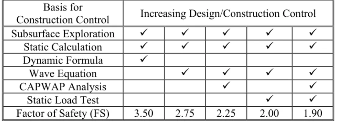
Under ASD, the FS is a summary of the engineer’s best estimate in the uncertainty associated in determining the actual structural loads, material strengths, potential failure modes, geotechnical strength parameters, and so forth (Becker, 1996). Traditionally, different magnitudes of FS have been used to reflect the different levels of control in foundation design and construction. Presumably, when more reliable methods are used to establish a higher level of control, a smaller FS can be used. This smaller FS, in turn, leads to a more economical design (Paikowsky, 2004). Table 2.1 reflects the minimum value of FS permitted by AASHTO (2004) for the ultimate axial geotechnical capacity of driven piles based on the level of construction control (Withiam, 2003).
The primary advantage of ASD is its simplicity. A number of weaknesses, however, have been cited with regard to its approach in designing driven piles. For example, “analyses varying in quality and/or quantity cannot be incorporated directly into reduction of the required FS for design” (Rahman et al., 2002). Essentially, more intensive subsurface exploration or laboratory testing programs do not necessarily result in the ability to use a smaller FS. Additionally, ASD also does not associate different degrees of uncertainty with both the estimated loads on the structure and its available resistance. As a result, different probabilities of failure may correspond to the same FS.
Table 2.1 Factor of Safety Based on Level of Construction Control (AASHTO, 2004)
Basis for
Construction Control Increasing Design/Construction Control
Subsurface Exploration
Static Calculation
Dynamic Formula
Wave Equation
CAPWAP Analysis
Static Load Test
Factor of Safety (FS) 3.50 2.75 2.25 2.00 1.90
2.4.2.Load and Resistance Factor Design (LRFD). Load and Resistance Factor Design (LRFD) is an alternative design method that has been progressively developed specifically for bridges since the mid-1980s. LRFD was well established in design codes around the world for structural engineering, but was first adopted in North America by the American Concrete Institute (ACI) Code in 1953 (DiMaggio et al. 1999). The objective of LRFD is to produce engineering designs with consistent levels of reliability using procedures from probability theory to ensure a prescribed margin of safety (Paikowsky, 2004).
Under LRFD, the uncertainties in loading are assessed separately from the uncertainties in resistance through a series of partial factors. These factors are known as load factors and resistance factors. The use of separate factors is a more rational approach than the use of a single FS (as in ASD) because loads and resistances have considerably separate and unrelated sources of uncertainty (Becker, 1996). For instance, the nominal loads of a structure are significantly influenced by the uncertainty related to estimating their magnitude; their influence has little impact on the uncertainty associated with evaluating the subsurface conditions that are providing resistance. Therefore, through LRFD, the design is not “penalized” for any uncertainties that pertain primarily to either the nominal load or the resistance (as it is in ASD).
Load factors, (typically those greater than 1) are used to account for the inherent uncertainties in determining the magnitude of the structural loads (dead load, live load, wind load, and so forth). In contrast, resistance factors (usually those less than 1) are
used to account for the uncertainty in individual resistance components (e.g., shaft resistance and end bearing) caused by such factors as soil behavior during different modes of failure, model specifications, and variations in soil conditions (Yoon, 2011). The LRFD criteria is expressed by the following equation:
(2.6)
where LF is the load factors, Qn is the nominal loads, RF is the resistance factor, and Rn is the nominal resistance.
By applying the load factors and resistance factors, the engineer is, in effect, over-estimating the structure’s loads and underestimating the structure’s strength. The primary advantage of LRFD is that it allows a more consistent, uniform level of safety. This, in turn, produces a more economical, repetitive design.
AASHTO published the first edition of LRFD bridge specifications in 1994. This new LRFD specification contained comprehensive design and construction guidance for both structural and geotechnical features. Initial use of the new specification, however, revealed showed that the approach used in LRFD for bridge superstructures (structural engineering design) was not fully compatible with the needs of bridge substructures (geotechnical engineering design). The primary disadvantage stems from the uncertainties in external loads being relatively small when compared with the uncertainties in strength-deformation behaviors of soils (DiMaggio et al., 1999). As a result, many geotechnical engineers reverted back to the ASD method of designing foundations they were accustomed to using in the past.
When structural engineers used the LRFD method to design a bridge’s superstructure, engineers struggled when designing the substructure with ASD because the critical load conditions were defined differently for the two procedures (Goble, 1996). Implementing different design methods for superstructures and substructures not only created uneconomical designs but also decreased the reliability of the designs that were constructed.
To ensure consistency between design methods, AASHTO and the Federal Highway Administration (FHWA) together issued a policy memorandum requiring all new bridges initiated after October 1, 2007 to be designed using the LRFD approach (Densmore, 2000). Resistance factors included in the LRFD specifications were calibrated using the FHWA developed Deep Foundation Load Test Database (DFLTD). The DFLTD consists of load test data for 1307 deep foundations collected between the years of 1985 and 2003 from all over the world. Following the mandate, concern rose that the nationally developed resistance factors were overly conservative when applied to localized regions because of the variability in not only the geology but also the construction practices used to calibrate them. For this reason, AASHTO permitted state Departments of Transportation (DOTs) to develop their own resistance factors based on regional practices and geology to minimize the unnecessary conservatism built into a design.
2.5.VARIOUS STATES LRFD IMPLENTATION EFFORTS
Following the release of the first edition of LRFD Bridge Specifications (1994) multiple state DOTs, including Florida, Pennsylvania, and Washington, began aggressively developing plans to fully implement LRFD.
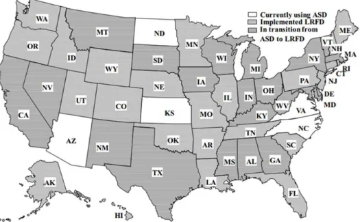
Following the imposed October 1, 2007 deadline, a number of surveys were conducted to determine the extent of LRFD state DOTs had implemented in bridge foundation design. AbdelSalam (2010) found that approximately 52% of the respondents were fully implementing LRFD, 33% were in a transition stage from ASD to LRFD, and the remaining 15% were still using ASD with FS between 2 and 2.5. Many of the states either implementing LRFD or in transition from ASD to LRFD initiated research programs to develop their own regionally calibrated LRFD resistance factors for foundation designs. Florida, Illinois, Louisiana, Wisconsin, and Iowa each published notable studies recommending LRFD resistance factors for driven pile foundations. The following sections will briefly summarize select efforts of multiple state DOTs to develop resistance factors for use within their respective states. Figure 2.1 illustrates the implementation status of each state as determined by AbdelSalam (2010).
Figure 2.1 Extent of LRFD Implementation Following Oct. 1, 2007 Deadline (AbdelSalam, 2010)
2.5.1. Florida. The Florida Department of Transportation (FDOT) began
training its engineers to incorporate LRFD after the original specification became available in 1994. Like most state DOTs, Florida recognized the over-conservatism built into the AASHTO recommended resistance factor. Resistance factors, however, were not included in AASHTO specifications for the common pile design software used by FDOT. Thus, FDOT was particularly interested in developing resistance factors based on the common geotechnical practices currently used in that state. In 1995, FDOT presented a plan to implement LRFD through the state’s specifications by 1998. FDOT outlined the process to fully implement LRFD specifications in the following steps:
1. Convert all design documents to LRFD
2. Modify all software to reflect LRFD environments
Both FDOT and the University of Florida (UF) used a series of pile load test databases progressively developed at UF since 1989 to calibrate geotechnical resistance factors for use in the state of Florida. The UF pile load test database for driven piles, entitled PILEUF, included data collected from over 72 different sites and more than 180 different tests (both End-of Drive and Beginning of Restrike) conducted across Florida (McVay, 2000).
FDOT recently initiated several research efforts focused on calibrating resistance factors for new foundations types. FDOT plans to continuously adjust and refine the calibrated resistance factors as more data becomes available. McVay et al. (2000) presented detailed information on this study, including pile data, statistical analysis, and the development of resistance factors.
2.5.2. Illinois. Previously, the Illinois Department of Transportation (IDOT)
estimated pile lengths using static analysis methods. The final pile length, however, was determined with a dynamic formula that was based on the pile driving resistance as determined in the field (Long et al, 2009a). Using separate methods to establish the design and acceptance criteria often resulted in a significant difference between the estimated lengths and actual pile lengths installed. For this reason, the Illinois Center of Transportation (ICOT) performed a study to evaluate IDOTs methods for predicting pile resistance and length. The objective of this research was to define the abilities of each predictive method, provide improvement if possible, and develop a calibrated series of resistance factors for the most reliable methods to be used in IDOT’s LRFD specifications.
ICOT developed and analyzed three separate databases of driven pile data to quantify the agreement between evaluated methods (Long et al, 2009). These databases included the International Database (a composite database of pile data used in several different studies), the Comprehensive Database (a database of 26 static pile load test records), and the IDOT Database (a database of piles only driven by IDOT). The analysis was used to not only identify but also correct the most accurate predicative methods for predicting pile resistance, including: combinations of static methods and dynamic formulas, pile type, and soil type. Findings from this study resulted in a series of LRFD resistance factors developed for the most reliable predicative methods. For
detailed information of this study, including pile data, statistical analysis, and the development of resistance factors, refer to Long et al. (2009a).
2.5.3.Louisiana. The Louisiana Department of Transportation and Development (LADOTD) began considering the use of LRFD specifications in 1995 but did not fully implement the method until 2005 (Yoon et al, 2008). Initially, LADOTD began using LRFD on select local projects by applying the national resistance factors suggested by AASHTO. As the familiarity and confidence in using LRFD increased, both LADOTD and the Louisiana Transportation Research Center (LTRC) initiated a research effort to calibrate regional geotechnical resistance factors for driven piles. This effort consisted of an extensive search of historical pile load test records collected within Louisiana. The search itself was limited to the installation records of containing both adequate subsurface information and a static load test performed to failure. The results of the search yielded 42 pile load tests that met these criteria. The soil boring information, pile driving logs, dynamic testing and analysis, static load test results were organized into a driven pile database. Using the collected data, LADOTD developed a series of resistance factors for various static and dynamic methods to be used within Louisiana. The resulting LADOTD resistance factors were 25 to 60 percent greater than the AASHTO recommended resistance factors, with an equivalent factor of safety at approximately 2.6 for the static methods analyzed.
As a result of their research program, LADOTD has currently initiated a major effort to not only write a geotechnical design manual but also rewrite the 2006 Louisiana Standard Specification for Roads and Bridges. In the future, LADOTD intends to continue improving their LRFD design and calibration for various methods and tests. They also hope to improve the state’s code to account for the new methods of contracting, construction, and ownership needed to properly implement LRFD. For detailed information, including the various static methods considered, statistical characterization performed, and LRFD resistance factors developed, refer to Yoon et al. (2008).
2.5.4. Wisconsin. In the past, the Wisconsin Department of Transportation (WisDOT) often drove piling in the field based on the Engineering News (EN) dynamic formula. The Federal Highway Administration (FHWA), however, has encouraged state
DOTs to migrate away from the EN Formula and toward a more accurate dynamic formula known as the FHWA-modified Gates formula (Long et al., 2009b). As a result, the University of Illinois initiated a study through the Wisconsin Highway Research Program to assess the use of both the Gates formula and other dynamic formulas in WisDOT practice.
Several datasets were collected and organized into two databases to provide a quantitative comparison of the predictive methods. The first database contained data from several smaller load test databases collected from various locations across the United States. The dataset collected for the nationwide database was limited to historical installation records of h-piles, pipe piles, and metal shell piles. It included static pile load test data and provided sufficient information to predict pile resistance using various dynamic formulae (if dynamic analysis was not already provided). A total of 156 records were compiled within this database.
The second database was created from the installation records of 316 piles driven exclusively by WisDOT. In some cases, CAPWAP (BOR) predictions were available. Very few records, however, included static pile load test data. At a minimum, each installation record included in this database was required to include the appropriate data needed to estimate the nominal resistance from simplistic dynamic formulas.
These program findings resulted in a new series of resistance factors for three commonly used WisDOT dynamic formulas. These new factors exceeded the values provided in the AASHTO (2010) specification by between 20 and 50 percent. For detailed information of this study, including the pile datasets, statistical analyses, and resulting resistance factors, refer to Long et al. (2009b).
2.5.5.Iowa. Historically, the Iowa Department of Transportation (IowaDOT) has aggressively collected static pile load test data. According to Roling et al. (2011), this data includes information from 264 pile static load tests conducted over a 24 year period (between 1966 and 1989) on steel H-piles, timber, pipe, monotone, and concrete piles. In 2005 IowaDOT and Iowa State University conducted a joint research project directed at the development of LRFD procedures for driven piles in IowaDOT bridges. This study focused on creating an electronic database of the historical IowaDOT pile load tests data to allow for the calibration of LRFD regional resistance factors.
The electronic database PIle-LOad Tests (PILOT) was developed using
Microsoft AccessTM to organize the available IowaDOT static load tests records.
Currently, PILOT contains 274 records of static pile load tests, varying in pile type and geological conditions, performed in Iowa. Researchers at Iowa State University surveyed both different state DOTs and Iowa county engineers to identify the most common, well-performing dynamic pile driving formulas. They then calibrated geotechnical resistance factors according to their response using the information available in PILOT. In all cases, the new series of calibrated resistance factors either equaled or exceeded the resistance factors recommended in the AASHTO (2010) specifications.
This compilation of available data into an electronic database allows IowaDOT designers and researchers the opportunity to access not only the quality but also the quantity of data needed for the accurate, effective calibration of regional LRFD resistance factors. For detailed information of both the methods evaluated and the determined results in this study, refer to AbdelSalam et al. (2008) and Roling et al. (2011).
2.6.MISSOURI LRFD IMPLEMENTATION EFFORTS
MoDOT adopted the national resistance factors found in the AASHTO LRFD Bridge Design Specifications Manual (2007) to design bridge foundations according to the FHWA mandate imposed in 2007. These specifications allow state DOTs to develop resistance factors based on their own regional practices and geology. To take advantage of this provision, MoDOT initialed its first research project to optimize design from both an economic and safety point of view.
2.6.1.Former Research Projects. In 2008, researchers from both Missouri University of Science and Technology (Missouri S&T) and the University of Missouri (Columbia) began the first MoDOT supported research program to develop a series of regional resistance factors for use within the state. These researchers used existing data from historical construction records on dynamic pile testing (i.e., Pile Driver Analyzer [PDA] and CAse Pile Wave Analysis Program [CAPWAP] software) to develop a new set of resistance factors for the static methods used by MoDOT. These factors were to