THÈSE
En vue de l’obtention duDOCTORAT DE L’UNIVERSITÉ DE TOULOUSE
Délivré par :Université Toulouse III Paul Sabatier (UT3 Paul Sabatier) Discipline ou spécialité :
Intelligence Artificielle
Présentée et soutenue par : Alexandre NIVEAU
le :27 mars 2012 Titre :
Knowledge Compilation for Online Decision-Making: Application to the Control of Autonomous Systems
École doctorale :
Mathématiques Informatique Télécommunications (MITT) Unité de recherche :
ONERA/DCSD/CD — IRIT/ADRIA Directeurs de Thèse :
Hélène FARGIER directrice de recherche CNRS IRIT, Université Paul Sabatier
Cédric PRALET ingénieur de recherche ONERA/DCSD Toulouse
Gérard VERFAILLIE directeur de recherche ONERA/DCSD Toulouse
Rapporteurs :
Enrico GIUNCHIGLIA professeur DIST, Università di Genova
Pierre MARQUIS professeur CRIL, Université d’Artois
Membres du jury :
Martin COOPER professeur IRIT, Université Paul Sabatier
submitted to the
University of Toulouse
in partial fulfillment of the requirements for the degree of
DOCTOR OF PHILOSOPHY
in Computer Science, specialty: Artificial Intelligence
delivered by theToulouse III–Paul Sabatier University (EDMITT)
Knowledge Compilation for Online
Decision-Making: Application to
the Control of Autonomous Systems
Presented and defended by
Alexandre NIVEAU
on March the 27th, 2012
Advisors:
Hélène FARGIER dir. de recherche CNRS Paul Sabatier University
Cédric PRALET ingénieur de recherche ONERA Toulouse
Gérard VERFAILLIE directeur de recherche ONERA Toulouse
Dissertation Examiners:
Enrico GIUNCHIGLIA professor University of Genova
Pierre MARQUIS professor University of Artois
Jury Members:
Martin COOPER professor Paul Sabatier University
Philippe JÉGOU professor Paul Cézanne University
This document was typeset using X E LATEX and the TEXLive library. Thanks to all contributors. Version 2.2.1-en, compiled October 15, 2012.
without whom I would, undoubtedly, still be in the process of writing Chapter 1.
Controlling autonomous systems requires to make decisions depending on cur-rent observations and objectives. This involves some tasks that must be executed online—with the embedded computational power only. However, these tasks are generally combinatory; their computation is long and requires a lot of memory space. Entirely executing them online thus compromises the system’s reactivity. But entirely executing them offline, by anticipating every possible situation, can lead to a result too large to be embedded. A tradeoff can be provided by knowledge compilation techniques, which shift as much as possible of the computational effort before the system’s launching. These techniques consists in a translation of a prob-lem into some language, obtaining a compiled form of the probprob-lem, which is both easy to solve and as compact as possible. The translation step can be very long, but it is only executed once, and offline. There are numerous target compilation languages, among which the language of binary decision diagrams (BDDs), which have been successfully used in various domains of artificial intelligence, such as model-checking, configuration, or planning.
The objective of the thesis was to study how knowledge compilation could be applied to the control of autonomous systems. We focused on realistic planning problems, which often involve variables with continuous domains or large enumer-ated domains (such as time or memory space). We oriented our work towards the search for target compilation languages expressive enough to represent such prob-lems.
In a first part of the thesis, we present various aspects of knowledge compi-lation, as well as a state of the art of the application of compilation to planning. In a second part, we extend the BDD framework to real and enumerated variables, defining the interval automata (IAs) target language. We draw the compilation map of IAs and of some restrictions of IAs, that is, their succinctness properties and their efficiency with respect to elementary operations. We describe methods for compil-ing into IAs problems that are represented as continuous constraint networks. In a third part, we define the target language of set-labeled diagrams (SDs), another generalization of BDDs allowing the representation of discretized IAs. We draw the compilation map of SDs and of some restrictions of SDs, and describe a method for compiling into SDs problems expressed as discrete continuous networks. We experimentally show that using IAs and SDs for controlling autonomous systems is promising.
Keywords
You would not be reading this thesis but for a number of people, whom I thank wholeheartedly. First of all, I owe a deep gratitude to my advisors Hélène Fargier, Cédric Pralet, and Gérard Verfaillie, for their amazing availability and dedication,1 for having patiently spurred on my work, leaving me all latitude to go in the direc-tions I wanted without imposing anything—and of course for having proofread this thesis (multiple times).
I am also grateful to all members of the jury: Enrico Giunchiglia and Pierre Marquis, who accepted the burden of being dissertation examiners; Martin Cooper, who presided the committee, and made numerous corrections and suggestions to the text; Philippe Jégou, who helped me relax during the defense by asking ques-tions in French; and Bruno Zanuttini, whose enthusiasm was much appreciated. Also, special thanks to Pierre, if only for having insightfully answered many of my questions about compilation throughout my PhD.
Furthermore, I am thankful to Christophe Garion, Thomas Schiex, and Florent Teichteil-Königsburg for their helpful comments and advice on the occasion of my first-year thesis committee. I owe a lot to Christophe, since he is also the one who introduced me to formal logic, who organized the introductory SUPAERO courses thanks to which I discovered artificial intelligence, and who suggested that I contact Cédric and Gérard for my Master research project.
I would like to offer my regards to people working at ONERA Toulouse, and in particular to thank secretaries and librarians, not only at ONERA but also at IRIT and at the university, for having made my life easier. Thanks to the PRES and ONERA for having awarded me the stipend thanks to which I could carry out my work; also, I stand indebted to people at the CRIL and the IUT de Lens for their warm welcome during the final months of my writing of this dissertation.
Thanks to all students whom I met during my Master and PhD at the ONERA-DCSD. I hold you greatly responsible for having made these years a quite enjoyable experience. I cannot afford being exhaustive—I would necessarily forget someone anyway; but I wanted to at least cite Caroline, Julie, Mario, Pascal, Prof. Jacquet,
you just won a beer; drop me an email. Among these, special thanks to Simon for his invaluable help with the cover, to Damien the little delivery boy, and to the mailmen Thibs and Simon (again).2 Rest assured that I will not hesitate to exploit you again in the future.
Last but not least, I am utterly grateful to my family for a fair numbers of rea-sons, among which having encouraged my curiosity, and simply having been there when I needed it (and also when I thought I did not). Above all, thanks to my wife for her patience, wisdom, and unqualified support.
2
While I am at it, let me stress that this work owes nothing at all to the following people: Ben, François, Paul, and Rod.
Introduction 1
I Context 3
1 Knowledge Compilation 5
1.1 Presentation . . . 5
1.1.1 Concepts and History . . . 5
1.1.2 Example of a Target Language: OBDDs . . . 7
1.2 A Framework for Language Cartography . . . 11
1.2.1 Notation . . . 12
1.2.2 Representation Language . . . 13
1.2.3 Language Comparison . . . 17
1.3 Boolean Languages . . . 22
1.3.1 General Rooted DAG Languages . . . 23
1.3.2 Fragments Based on Operator Restrictions . . . 27
1.3.3 “Historical” Fragments . . . 28
1.3.4 Fragments Based on Node Properties . . . 30
1.3.5 The Decision Graph Family . . . 30
1.3.6 Ordering for Decision Graphs . . . 34
1.3.7 Closure Principles . . . 36
1.4 Compilation Map of Boolean Languages . . . 37
1.4.1 Boolean Queries and Transformations . . . 37
1.4.2 Succinctness Results . . . 43
1.4.3 Satisfaction of Queries and Transformations . . . 44
1.5 Non-Boolean Languages . . . 45 1.5.1 ADDs . . . 46 1.5.2 AADDs . . . 47 1.5.3 Arithmetic Circuits . . . 48 1.5.4 A Unified Framework: VNNF . . . 49 1.6 Compiling . . . 49
1.6.1 Compilation Methods . . . 50
1.6.2 Existing Compilers: Libraries and Packages . . . 53
1.7 Applications of Knowledge Compilation . . . 54
1.7.1 Model Checking . . . 54 1.7.2 Diagnosis . . . 57 1.7.3 Product Configuration . . . 58 2 Planning 61 2.1 General Definition . . . 61 2.1.1 Intuition . . . 61
2.1.2 Description of the World . . . 62
2.1.3 Defining a Planning Problem . . . 64
2.1.4 Solutions to a Planning Problem . . . 66
2.2 Planning Paradigms . . . 69
2.2.1 Forward Planning in the Space of States . . . 70
2.2.2 Planning as Satisfiability . . . 70
2.2.3 Planning as Model-Checking . . . 72
2.2.4 Planning Using Markov Decision Processes . . . 72
2.2.5 More Paradigms . . . 74
2.3 Knowledge Compilation for Planning . . . 75
2.3.1 Planning as Satisfiability . . . 75
2.3.2 Planning as Heuristic Search . . . 77
2.3.3 Planning as Model-Checking . . . 77
2.3.4 Planning with Markov Decision Processes . . . 79
3 Orientation of the Thesis 81 3.1 Benchmarks . . . 81
3.1.1 Drone Competition Benchmark . . . 81
3.1.2 Satellite Memory Management Benchmark . . . 82
3.1.3 Transponder Connections Management Benchmark . . . . 83
3.1.4 Attitude Rendezvous Benchmark . . . 83
3.2 A First Attempt . . . 84
3.2.1 Our Approach to theDroneProblem . . . 84
3.2.2 Results for theDroneproblem . . . 86
3.3 Towards More Suitable Target Languages . . . 86
3.3.1 General Orientation . . . 86
3.3.2 Identifying Important Operations . . . 86
3.3.3 New Queries and Transformations . . . 87
II Interval Automata 91
4 Interval Automata Framework 95
4.1 Language . . . 95
4.1.1 Definition . . . 95
4.1.2 Interval Automata . . . 96
4.1.3 Relationship with theBDDfamily . . . 98
4.1.4 Reduction . . . 99
4.2 Efficient Sublanguage . . . 103
4.2.1 Important Requests on Interval Automata . . . 103
4.2.2 Focusingness . . . 104
4.3 The Knowledge Compilation Map ofIA . . . 106
4.3.1 Preliminaries . . . 106
4.3.2 Succinctness . . . 109
4.3.3 Queries and Transformations . . . 110
4.4 Chapter Proofs . . . 112
4.4.1 Reduction . . . 112
4.4.2 Sublanguages . . . 113
4.4.3 Preliminaries to the Map . . . 116
4.4.4 Queries and Transformations . . . 121
5 Building Interval Automata 127 5.1 Continuous Constraint Networks . . . 127
5.2 Bottom-up Compilation . . . 128
5.2.1 Union of Boxes . . . 128
5.2.2 Combining Constraints . . . 129
5.3 RealPaver with a Trace . . . 129
5.3.1 RealPaver’s Search Algorithm . . . 129
5.3.2 Tracing RealPaver . . . 130
5.3.3 Taking Pruning into Account . . . 132
5.3.4 Example . . . 134
5.3.5 Properties of Compiled IAs . . . 134
6 Experiments on Interval Automata 137 6.1 Implementation . . . 137
6.1.1 Experimental Framework . . . 137
6.1.2 Interval Automaton Compiler . . . 137
6.1.3 Operations on Interval Automata . . . 138
6.2 Compilation Tests . . . 139
6.3 Application Tests . . . 140
6.3.1 Simulating Online Use of theDroneTransition Relation . 140 6.3.2 Simulating Online Use of theSatelliteSubproblem . . . . 143
III Set-labeled Diagrams 145
Back to Enumerated Variables 147
Remarks about Meshes and Discretization . . . 147
Discrete Interval Automata . . . 148
7 Set-labeled Diagrams Framework 151 7.1 Language . . . 151
7.1.1 Definition . . . 151
7.1.2 Reduction . . . 153
7.2 Sublanguages of Set-labeled Diagrams . . . 154
7.2.1 TheSDFamily . . . 154
7.2.2 Relationship with theIAandBDDFamilies . . . 155
7.3 From IAs to SDs . . . 157
7.3.1 A Formal Definition of Discretization . . . 158
7.3.2 Transforming IAs into SDs . . . 159
7.4 The Knowledge Compilation Map ofSD . . . 160
7.4.1 Preliminaries . . . 161
7.4.2 Succinctness . . . 162
7.4.3 Queries and Transformations . . . 165
7.5 Chapter Proofs . . . 167
7.5.1 Reduction . . . 167
7.5.2 Relationship with Other Languages . . . 168
7.5.3 Discretization of IAs . . . 168
7.5.4 Preliminaries to the Map . . . 170
7.5.5 Succinctness . . . 179
7.5.6 Queries and Transformations . . . 184
8 Building Set-labeled Diagrams 199 8.1 Discrete Constraint Networks . . . 199
8.2 Bottom-up Compilation . . . 200
8.3 CHOCO with a Trace . . . 201
8.3.1 CHOCO’s Search Algorithm . . . 201
8.3.2 Tracing CHOCO . . . 202
8.3.3 Caching Subproblems . . . 203
8.3.4 Properties of Compiled SDs . . . 206
9 Experiments with Set-labeled Diagrams 207 9.1 Implementation . . . 207
9.1.1 Experimental Framework . . . 207
9.1.2 Set-labeled Diagrams Compiler . . . 208
9.1.3 Operations on Set-labeled Diagrams . . . 208
9.2 Compilation Tests . . . 209
9.3.1 Simulating Online Use of a Transition Relation . . . 210 9.3.2 Simulating Online Use of theTelecomBenchmark . . . . 212
Conclusion 213
A Benchmark Specifications 217
A.1 Droneproblem . . . 217 A.2 Telecom . . . 222
Bibliography 225
1.1 Example of a BDD . . . 8
1.2 Examples of an FBDD and an OBDD . . . 9
1.3 Example of an MDD . . . 9
1.4 Reduction of a BDD . . . 10
1.5 Example of a GRDAG . . . 25
1.6 Decision node and its simplified representation . . . 31
1.7 A GRDAG satisfying weak decision, and its simplified representation 32 1.8 Example of a DG . . . 34
1.9 Example of a BED . . . 35
1.10 Succinctness graph of someNNFSBB fragments . . . 43
1.11 Example of a Kripke structure . . . 54
2.1 Elements of a planning problem . . . 63
2.2 A state-transition system defined with fluents . . . 65
3.1 Example of an OBDD policy for theDroneproblem . . . 85
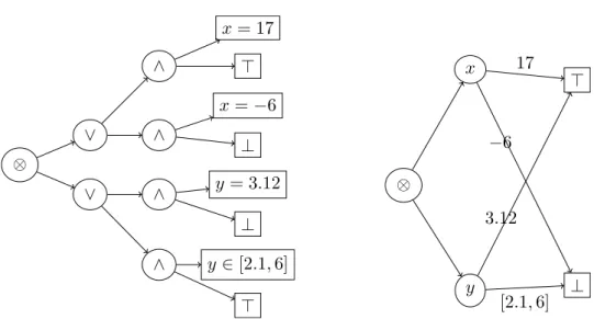
4.1 Example of an interval automaton . . . 97
4.2 Merging of isomorphic nodes . . . 99
4.3 Elimination of an undecisive node . . . 100
4.4 Merging of contiguous edges . . . 100
4.5 Merging of a stammering node . . . 101
4.6 Elimination of a dead edge . . . 101
4.7 Example of a non-empty inconsistent IA . . . 104
4.8 Example of an FIA . . . 104
4.9 Meshes induced by an IA . . . 109
4.10 Succinctness graph of theIAfamily . . . 111
5.1 Result of “RealPaver with a trace” on a given CCN . . . 134
5.2 Illustration of how “RealPaver with a trace” treats enumerated vari-ables . . . 135
6.1 Illustration of the expressivity ofIA . . . 147
6.2 IAs with various levels of precision . . . 148
6.3 Discretizing arbitrarily or adaptively . . . 149
7.1 Example of SD . . . 152
7.2 Illustration of the new definition of stammeringness . . . 153
7.3 Hierarchy of theSDfamily . . . 155
7.4 Comparison of the reduction of an SDSZE -representation as an IA and as an SD . . . 156
7.5 Succinctness graph of theSDfamily . . . 164 7.6 OSDDs for the star coloring problem with different variable orders 165
1.1 Queries satisfied by fragments ofNNFSBB . . . 44
1.2 Transformations satisfied by fragments ofNNFSBB . . . 45
3.1 Number of nodes of various OBDDs for six instances of theDrone problem . . . 85
4.1 Queries satisfied byIAandFIA . . . 111
4.2 Transformations satisfied byIAandFIA . . . 111
4.3 Proofs ofIA’s andFIA’s satisfaction of queries . . . 125
4.4 Proofs ofIA’s andFIA’s satisfaction of transformations . . . 125
6.1 Results about the compilation of RealPaver’s output intoFIA . . . 139
6.2 Results of “RealPaver with a trace” experiments . . . 140
6.3 Results ofFIAexperiments on theDronebenchmark, Scenario 1 . 140 6.4 Results ofFIAexperiments on theDronebenchmark, Scenario 2 . 142 6.5 Results ofFIAexperiments on theDronebenchmark, Scenarios 3 and 4 . . . 142
7.1 Succinctness results for theSDfamily . . . 164
7.2 Queries satisfied by fragments ofSD . . . 166
7.3 Transformations satisfied by fragments ofSD . . . 166
7.4 Proofs of the succinctness of theSDfamily . . . 184
7.5 Proofs ofSDfragments’ satisfaction of queries . . . 197
7.6 Proofs ofSDfragments’ satisfaction of transformations . . . 198
9.1 Results of “CHOCO with a trace” experiments . . . 209
9.2 Results ofFSDDexperiments on theDroneandObsToMem bench-marks, Scenario 1 . . . 210
9.3 Results ofFSDDexperiments on theDroneandObsToMem bench-marks, Scenario 2 . . . 211
9.4 Results ofFSDDexperiments on theDroneandObsToMem bench-marks, Scenarios 3 and 4 . . . 211 9.5 Results ofFSDDexperiments on theTelecombenchmark . . . 212
2.1 Forward state-space search for solving planning problems . . . 70
2.2 Online “planning as SAT” procedure used by Barrett [Bar03] . . . 76
2.3 Conformant planner of Palacios et al. [PB+05] . . . 77
2.4 Weak planning as model-checking algorithm with forward search . 78 2.5 Strong planning as model checking algorithm with backward search 79 4.1 Reduction of IAs . . . 102
4.2 Conditioning of an IA . . . 103
4.3 Model extraction on an FIA . . . 106
4.4 Context extraction on an FIA . . . 107
4.5 Term restriction on an FIA . . . 117
4.6 Conjunction of an FIA and a term . . . 124
5.1 RealPaver’s search algorithm . . . 130
5.2 Simplified “RealPaver with a trace” . . . 131
5.3 Complete “RealPaver with a trace” . . . 133
7.1 Transformation of IAs into SDs (discretization) . . . 160
7.2 Validity checking onFSDD . . . 162
7.3 Computation of the negation of an SDD . . . 163
7.4 Translation of a term intoOSDD< . . . 171
7.5 Translation of a clause intoOSDD< . . . 171
7.6 Conjunction onOSD< . . . 189
7.7 Equivalence checking onOSDD . . . 192
7.8 Construction of an SD used to proveNP-hardness of several trans-formations . . . 194
8.1 CHOCO’s search algorithm . . . 202
8.2 Basic “CHOCO with a trace” . . . 203
A system (vehicle, instrument) isautonomous if it is not controlled by a human operator. Its actions are driven by an inner program, which is not modified while the system is working; the program isembeddedinto the system, and allows it to “make decisions” all by itself. Embedded systems are generally subject to a lot of limitations (such as price, weight, or power) that depend on the specific task they have to handle. As a consequence, embedded systems do not have many resources at their disposal, in terms of memory space and computational power available onboard. However, they generally require highreactivity. These constraints are even more significant when dealing with embedded systems controlling aeronau-tical and spatial autonomous systems, such as drones or satellites: their resources can be severely limited, and lack of reactivity can be a crucial issue.
Decision-making is one of the targets of an artificial intelligence field, namely planning. To produce decisions fitting the situation, the program has to solve a planning problem. Tools have been designed in order to solve such problems; using these tools, the system can compute suitable decisions to make. However, in the general case, planning problems are hard to solve—they have a high computational complexity. The basic consequence of this fact is that making decisions by solving planning problems takes time, especially on autonomous systems, that have limited computational power. Reactivity is thus not ensured if the problem is solvedonline, i.e., each time it is needed, using only the system’s power and memory.
To settle this issue, one possibility is to compute decisionsoffline, that is, before the system is set up. Anticipating all possible situations, and solving the problem for each of them, we could provide the system with a decision table, containing a set of “decision rules” of the form “inthissituation, makethatdecision”. This would guarantee a maximal reactivity for the system, since using such a table online does not require a high computational power.
However, this enhancement in reactivity may imply an important increase in memory space. Indeed, decision-making depends on lots of parameters, includ-ing for instance measurements, current (supposed) position, state of components, current data, current objectives, and even some former values of these parameters. This leads to a huge number of possible situations, and thus to a huge number of
decision rules in the decision table, whereas the memory space available online is drastically limited.
We see that a compromise is necessary between reactivity and spatial compact-ness.Knowledge compilationis a way of achieving such a compromise: the objec-tive of this discipline is to study how one cantranslatea problem offline, to facil-itate its online resolution. It examines to what extenttarget languages, into which problems can becompiled, allow online requests to be tractable, while keeping the representation as compact as possible. Using knowledge compilation amounts to shifting as much computational effort as possible before the system’s setting up, thus obtaining good reactivity, while deteriorating space efficiency as little as pos-sible.
Knowledge compilation techniques have proven useful for various applications, including planning. The goal of this thesis was to study how it is possible to advan-tageously apply these techniques torealplanning problems related to aeronautical and spatial autonomous systems. We considered a number of real problems, and remarked in particular that the target languages used in state-of-the-art planners are not specifically designed to handle some aspects of our problems, namely continu-ous domains. We oriented our work towards the application of these state-of-the-art techniques to other (possibly new), more expressive target languages.
This thesis is divided into three parts. The first one develops thecontextof the work, detailing knowledge compilation [Chapter 1] and planning [Chapter 2]. It explains [Chapter 3] why we felt that our subject raised the need for new target compilation languages. The second part deals withinterval automata, one of the new languages we defined. It presents some theoretical aspects of this language [Chapter 4], details how we can build elements of this language in practice [Chap-ter 5], and provides experimental results [Chap[Chap-ter 6]. The third part is about an-other language we defined,set-labeled diagrams. Using a similar outline to that of Part II, it begins with definitions and general properties about the language [Chap-ter 7], presents our compilation algorithm [Chap[Chap-ter 8], and ends with experimental results [Chapter 9].
1
Knowledge Compilation
This chapter details the main topic of this work, namely knowledge compilation. In a nutshell, knowledge compilation consists in transforming a problem offline, in order to facilitate its online resolution. This transformation is actually considered as atranslationfrom the originallanguagein which the problem is described, into a target languagethat has good properties, to wit, allowing the problem to be solved “easily” while remaining as compact as possible.After having presented and illustrated the basic idea and concepts of knowledge compilation [§ 1.1], we formally define notions pertaining tolanguages[§ 1.2]. A number of state-of-the-art languages are then defined [§ 1.3]; they belong to the particular class of graph-based Boolean languages, on which we focused during the thesis. The next section details some properties of this class, and provides theoreti-cal results from the literature [§ 1.4]. We then give some insight about non-Boolean languages [§ 1.5]. The last two sections of the chapter are dedicated to practical as-pects of knowledge compilation [§ 1.6] and successful applications [§ 1.7].
1.1
Presentation
1.1.1
Concepts and History
Knowledge compilation can be seen as a form of “factorization”, since the offline phase is dedicated to executing computations that are bothhard andcommon to several online operations. This idea is not new, as illustrated by the example of tables of logarithms [Mar08]. These tables were used to facilitate hand-made calculations, at a time when calculators were not as small and cheap as today. They contain couples ⟨x,log10(x)⟩, for a lot of different real values ofx; these couples could then be used to make complex calculations, such as root extrac-tion. For example, calculating √9
9 √
876 = (8.76×10²)1/9, it holds that log10(√9876) =log10((8.76×10²)1/9) = (log10(8.76) + 2)/9. The user willing to get an approximate value of √9876only has to look up the value of log10(8.76) ≈ 0.942504106in the table, compute the fraction(0.942504106 + 2)/9 = 0.326944901(which is easy to do by hand), and look up the antecedent of0.326944901by log10in the table. The user then obtains that√9
876≈2.122975103, having used only simple operations.
This example fits the definition of knowledge compilation, even if the context is a bit different (knowledge compilation is not used to facilitatehandmade calcula-tions). Indeed, the offline phase consists in calculating logarithms, which are hard to obtainandpotentially useful for several online operations. Each entry can then be used in many different cases (the value of log10(8.76)can be used to compute the roots of876,87.6,8.76…), and for each case, the work left to the user is easy.
Let us take an example closer to our subject. In the introduction, the first solu-tion we proposed to tackle the quessolu-tion of autonomous systems’ reactivity was to solve the problem beforehand for all possible situations, providing the program with a table of decision rules. Albeit naive, this solution actually relies on knowledge compilation. We can identify the three main points of the definition: the offline phase proceeds with computations that are hard (solving the planning problem for multiple initial situations) and repeated over time (a given situation can be met mul-tiple times; the suitable decision is computed once and for all), and the online phase left to the system is simple (look up in the table the next decision to make).
What is usually (and historically) designated ascompilationis the translation of a program, from a high-level programming language, easily understandable and modifiable by human beings, to a low-level machine language, much more efficient from a computational point of view. This is also a case of pre-processing, in which we transform something offline to facilitate its online use. The specificknowledge compilationdomain differs from the general study of pre-processing in two ways.
First, following Marquis [Mar08], the name “knowledge compilation” tauto-logically limits it to “compilation of knowledge”: it deals with the translation of knowledge bases (that is, a set of pieces of information, generally represented as logic formulæ) and with the exploitation of this knowledge, i.e., automated rea-soning. The definition remains quite general—lots of things can be understood as “pieces of information”—but typically excludes the classical program compilation from the scope of knowledge compilation.
The second difference between standard compilation and knowledge compila-tion is a consequence of the previous one [CD97]. Being linked to knowledge rep-resentation and reasoning, knowledge compilation inevitably stumbles upon prob-lems considered hard with respect tocomputational complexity theory[see Pap94 for an overview], for example,NP-complete problems,Σp2-complete problems, or evenPSPACE-complete problems—all widely conjectured to not be solvable in polynomial time. The goal of researchers in knowledge compilation is not just to make a problemsimpler, but to make itdrasticallysimpler, by changing its com-plexity class to a more tractable one, for example fromNP-complete toP, from PSPACE-complete toNP, etc.
In Chapter 2, we show how solving a planning problem amounts to applying some operations on some functions. Our application, controlling autonomous sys-tems, requires a minimal online complexity; this is why we focused on the possible ways to achievepolynomialcomplexity for the online operations. This removes from our study a number of representations, on which polytime reasoning is not possible [e.g., the high-level logics listed in GK+95]. We basically limit ourselves to graph-based structures.
Research has been made to decide whether knowledge compilation is useful to some given reasoning problem. Roughly speaking, a problemP is considered compilable into a complexity classCif and only if there exists a compilation func-tion transformingP into another problemP′, such thatP′ is of size polynomial in the size ofP, andP′ is in classC. In other words, the compilation step may be really hard—there is no restriction on the time complexity of the compilation function—but the compiled form can take only polynomially more space than the original problem. Compilability has been formalized by Cadoli et al. [CD+96, for an extended review see CD+00].
Since we want our operations to be of polynomial complexity, it would seem that we are only interested in problemscompilable intoP, the complexity class of polytime problems. However, it has been proven by Liberatore [Lib98] that plan-ning (in itsclassicalform [§ 2.1.3.3]) isnotcompilable intoP. Trying to compile planning problems can nevertheless be useful for several reasons. First, this non-compilability result means that there can be no polysize compilation function trans-forminganyplanning problem into a tractable one; the compilation function must be common to all problems. It does not imply that a specific planning problem, when taken apart from the others, cannot be transformed into a tractable one. Sec-ond, the compilability framework only takesworst-case complexityinto account— it does not say anything about average or practical space complexity. Last, studying the compilation of subparts of planning problems could be worthwhile anyway.
Before moving on to a practical example of a target compilation language, let us also specify that this work only concerns knowledge compilation in the context of classical propositional inference; we did not study its application to the non-classical inference relations designed for reasoning under inconsistency. We will thus not consider stratified or weighted belief bases, though there exists some liter-ature regarding their compilation [BYD07, DM04].
1.1.2
Example of a Target Language: OBDDs
Compiling a problem is modifying its form (this modification being potentially hard to do), so that the problem in its compiled form is tractable, yet as compact as possible. This can be seen as atranslationfrom aninput languageinto atarget language. We give a formal definition of a “language” in the next section [§ 1.2]; before that, let us illustrate what it can look like and how it is generally handled, using the influential language ofordered binary decision diagrams, better known asOBDDs.
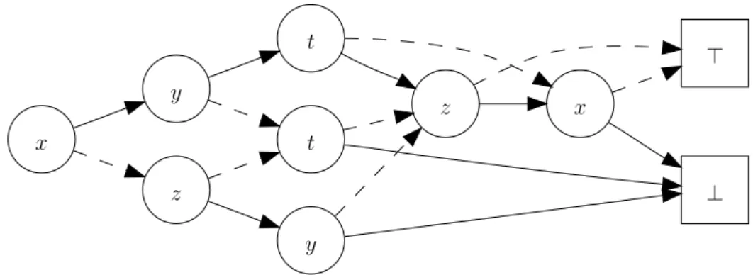
⊤ ⊥ x z t t y y z x
Figure 1.1: An example of a BDD. Solid (resp. dashed) edges are⊤-labeled ones (resp.⊥-labeled ones).
Binary Decision Diagrams
Introduced by Lee [Lee59] and Akers [Ake78],binary decision diagrams (BDDs) are rooted directed acyclic graphs that represent Boolean functions of Boolean variables. They have exactly two leaves, respectively labeled ⊤(“true”) and ⊥ (“false”); their non-leaf nodes are labeled by a Boolean variable and have exactly two outgoing edges, also respectively labeled⊤and⊥. Figure 1.1 gives an example of a BDD.
A BDD represents a function, in the sense that it associates a unique Boolean value with eachassignment of the variables it mentions. Let us illustrate this on the simple example of Figure 1.1. Four variables are mentioned; each one of them can take two values. If we choose one value for each variable, for examplex = ⊤, y = ⊥, z = ⊤, andt = ⊥, we get an assignment of these four variables, among the 24 = 16possible ones. How does the BDD associate a truth value with this assignment? To get the result, one simply has to start from the root, and follow a path to one of the leaves. The path is completely determined by the chosen assignment: to each node corresponds a variable, the next edge to cross being the one being labeled by the value assigned to this variable. The path ends up either at the⊤-leaf or at the⊥-leaf: the label is the value that the function associates with the chosen assignment.
The name “binary decision diagram” faithfully transcribes this behavior: start-ing from the root, each node corresponds to a possible decision—“which value do I choose for this variable?”—directing users to the subgraph fitting their choice—“if you decide this, go here, else go there”. Note that each possible assignment corre-sponds to exactly one path; BDDs thus representfunctions(and notrelations).
The “Decision Diagram” Family
By imposing structural restrictions on BDDs, we obtain interestingsublanguages. For example, afree BDD (FBDD)[GM94] is a BDD that satisfies the read-once property: each path contains at most one occurrence of each variable. But the most
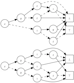
⊤ ⊥ z t y t t z y x ⊤ ⊥ t t z z z y y x
Figure 1.2: An FBDD (top) and an OBDD (bottom), both representing the same function as the BDD of Figure 1.1.
⊤ ⊥ w v u 2 3 1 3 1 2 2 1 3
Figure 1.3: An example of an MDD, over variablesu,v, andw, of domain{1,2,3}. influential kind of BDD is theordered BDD (OBDD)[Bry86], in which the order of variables is imposed to be the same in every path. Figure 1.2 shows an FBDD and an OBDD representing the same function as the BDD in Figure 1.1.
The concept of “decision diagram” is not inherently related to Boolean values; the idea has been extended to non-Boolean variables, yieldingmulti-valued decision diagrams (MDDs)[§ 1.3.6], and also to non-Boolean functions, yieldingalgebraic decision diagrams (ADDs)[§ 1.5.1]. Figure 1.3 gives an example of an MDD.
OBDDs Are Compact and Efficient
We showed what OBDDs are, and how they work; but why are they interesting as a knowledge compilation language? There are two simple informal reasons to this: they are efficient, and they are small. Of course, these two aspects are not dissociable. OBDDs are not the smallest possible representation of a function:
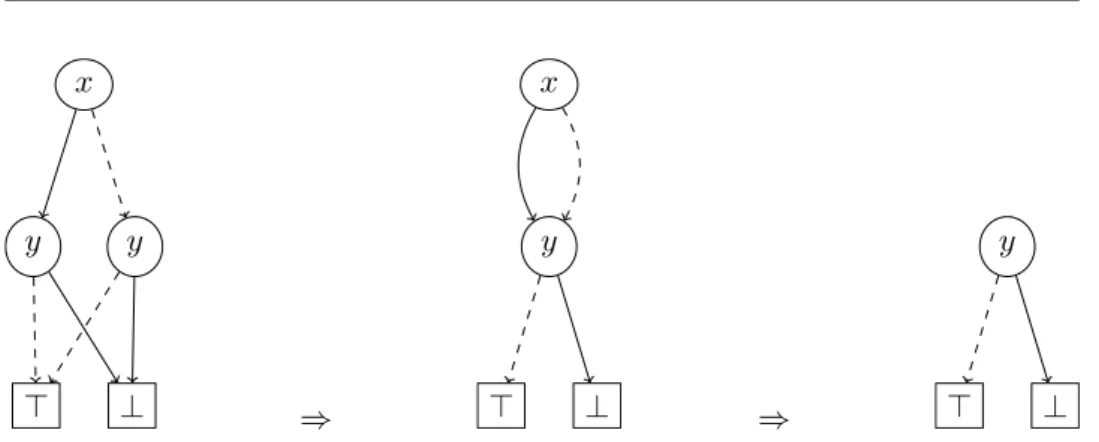
.. y . x .⊤ . y . ⊥ ⇒ .. y . x .⊤ . ⊥ ⇒ .. y .⊤ . ⊥
Figure 1.4: Illustration of the reduction procedure on binary decision diagrams. The BDD on the left represents formula (x∧ ¬y)∨(¬x∧ ¬y). The reduction procedure merges the twoy-nodes, which areisomorphic(they represent the same function); the result is the BDD in the middle. Then thex-node is removed, because it isredundant: the value ofxdoes not matter. The reduced BDD is on the right.
propositional formulæ are generally smaller. Neither are OBDDs the most efficient representations for all applications: computing the conjunction of several functions is easier using truth tables, for example. What is advantageous with OBDDs is that they arebothefficient and small—they are a good compromise between efficiency and size.
What makes OBDDs so small? The answer lies in their graph structure, that allowsfactorizationof “identical” subgraphs, i.e., subgraphs representing the same function—they are said to beisomorphic. This factorization can be done thanks to a polytime reduction procedure, described by Bryant [Bry86], and illustrated in Figure 1.4. Not only does this reduction procedure allow exponential gains in space for some cases, but it is also the key to the efficiency of OBDDs. The polynomiality of the reduction procedure is important; it indeed makes it possible to always work on reduced OBDDs. In the following, we always implicitly consider OBDDs to be reduced.
The efficiency of OBDDs is considered with respect to their performances on common, useful operations. Checking whether there exists an assignment satisfy-ing a propositional formula is hard, yet it can be done in constant time if the for-mula is represented as a reduced OBDD (the only OBDDs that have no satisfying assignment are those that can be reduced to the⊥-leaf). More importantly, check-ing whether two OBDDs uscheck-ing the same order of variables represent the exact same function can be done in time linear in the sum of the two OBDDs’ sizes. Moreover, building an OBDD representing the conjunction (or disjunction, or application of any Boolean operator) of two OBDDs using the same variable ordering is only lin-ear in the product of the sizes of the two OBDDs. These remarkable properties of OBDDs were discovered by Bryant [Bry86].
They are not the only language having such interesting properties: all the op-erations described have for example a linear worst-case complexity on truth
ta-bles. However, OBDDs have these properties while being potentially exponentially smaller than truth tables. Indeed, the memory size necessary to store a truth table is proportional to the number of satisfying assignments of the represented formula, whereas it is not the case for OBDDs.
OBDDs: The Best Language?
Being such a good compromise between spatial and operational efficiency, OBDDs have been widely used for multiple applications over the years. Does this mean they are the best structures to compile Boolean functions? The answer is generally no, because it depends on the target application. When one needs to often check whether two functions are equivalent, and often compute conjunctions, OBDDs are probably the best choice; but if the equivalence-checking test is superfluous, and all one needs is a model-checking test, the less constrained BDDs are much better, since they can take exponentially less memory space.
* * *
Choosing a language for one’s application is thus an important conception step, that must not be neglected, for a bad choice can lead to great loss in time or space performances—this is particularly crucial in the case of embedded systems. This is rendered difficult by the fact that there exists a lot of target languages, especially in the family of structures representing Boolean functions of Boolean variables. A user thus needstoolsto compare languages and make a good choice. Introduced by Darwiche and Marquis [DM02], theknowledge compilation mapprovides such tools; we present them in the following section.
1.2
A Framework for Language Cartography
The goal of theknowledge compilation mapis to compare languages according to their spatial complexity and their efficiency (in terms of worst-case complexity) for different possible operations, such as querying some information on the compiled form, or applying transformations. The map makes it easy to compare fragments from a theoretical complexity point of view, retaining only the best ones for a given application.
The purpose of this section is to present the knowledge compilation map frame-work. We formally define the notion oflanguage, and present the concepts that are used to compare languages—but prior to this, let us introduce our notation con-ventions. Note that an index of symbols is available at the very end of this thesis [p. 237].
1.2.1
Notation
We denote asRthe set of real numbers, asZthe set of integers, asNthe set of natural numbers (including0), asN∗the set of positive integers (excluding0), and asBthe set of Boolean constants. We use⊤and⊥to refer to the Boolean constants “true” and “false” respectively, but often implicitly identifyBwith{0,1}, so that the following inclusions hold:
B⊆N⊆Z⊆R.
We useSAto denote the set of singletons of a setA. Thus, for example,SB =
{
{⊤},{⊥}}, andSN=∪n∈N{{n}}.
For the sake of generalization, the variables we consider can have any kind of domain—discrete or continuous, finite or infinite…as long as it is not empty. We callV the set of all possible variables; V is of course non-empty, and we assume that it is ordered by some total strict order<V. When considering a set of sub-scripted variables, such as{x1, x2, . . . , xk}, it will always be implicitly supposed thatx1<V x2 <V . . . <V xk.
Forx ∈ V, we denote by Dom(x)itsdomain, which, from a general point of view, can be any non-empty set. Nevertheless, we often need to consider variables defined on specific domains: given a setS, we defineVS ={x ∈ V |Dom(x) =
S}. Important classes of variables include B, the set of Boolean variables (sim-ply defined as VB), and E, the set of enumerated variables, that we arbitrarily define as the set of all variables with a finite integer interval domain (formally, E=∪(a,n)∈Z×NV{a,a+1,...,a+n}).
ForX ={x1, . . . , xk} ⊆ V, Dom(X)denotes the set ofassignments of
vari-ables fromX (or X-assignments), that is, Dom(X) = Dom(x1)×Dom(x2)×
· · · ×Dom(xk). We denote as #—x anX-assignment, i.e., #—x ∈ Dom(X). SetX is called thesupportof#—x. The empty set can have only one assignment, denoted∅#—.
LetX, Y ⊆ V, and let #—x be an X-assignment. Therestrictionof #—x to the variables ofY, denoted #—x|Y, is theX∩Y-assignment in which each variable takes the same value as in#—x. Note that this definition allowsY to be disjoint fromX(in which case #—x|Y is always equal to∅#—). For a given variablexi ∈ X, #—x|{xi} thus
gives the value taken byxiin #—x; we simply denote it by#—x|xi.
LetX, Y ⊆ V, and let#—xand#—y be someX- andY-assignments. IfXandY are disjoint, #—x . #—y denotes theconcatenationof the two assignments, i.e. theX∪Y -assignment that coincides with #—x on variables fromX and with #—y on variables fromY.
GivenS andE some sets, we use the notationES to designate the set of all functions of the formf:S→E;Sis called theinput setoff, andEitsvaluation set. The restriction off to a set S′, denotedf|S′, is the function from S∩S′ to
E which coincides withf onS ∩S′. We generally consider functions verifying
S=Dom(V), withV ⊆ V some set of variables. We call them functions over the variables fromV to the setE. For such a functionf: Dom(V)→E,V is called thescopeoff, and is denoted Scope(f). Note that we authorize functions to take
as input assignments the support of which is larger than the scope of the function: it will always be implicitly considered thatf(#—v)meansf(#—v|Scope(f)).
1.2.2
Representation Language
Let us now introduce the basic elements of the map. At the highest level of abstrac-tion, these elements are calledrepresentation languages, and have been formalized in the propositional case by Fargier and Marquis [FM09]. We extend their definition here so that it captures all languages presented thereafter.1
What Is Expressed: Interpretation Domain
Generally speaking, knowledge compilation languages representfunctions. These functions are of various kinds: some languages are used to handle Boolean func-tions, some others to handle real-valued functions; some hold on Boolean variables, some others on enumerated variables. We say that they have differentinterpretation domains—an interpretation domain being the set of functions that are admissible in the language.
Definition 1.2.1(Interpretation domain).LetV ⊆ Vbe afiniteset of variables, and
Eany set. Theinterpretation domainassociated withV andEis the set
DV,E =
∪
V′⊆V
EDom(V′)
of the functions holding on some variables fromV and returning elements inE. For example,DB,B is the set of Boolean functions of Boolean variables; it is the interpretation domain of OBDDs [§ 1.1.2].
How It Is Expressed: Data Structures
Knowledge compilation aims at expressing functions as instances of specificdata structures. A data structure [see e.g. CL+01, Part III] is a particular organization of computer data, together with some algorithms allowing data to be handled effi-ciently, by taking advantage of this organization. Well-known data structures in-clude stacks, queues, hash tables, trees, graphs…
A mathematical object, such as a function, is an abstract concept. To represent it using data structures, it is necessary tomodel it, by identifying the basic oper-ations by means of which it is handled. For instance, setsare “things” one can intersect, unite, enumerate, etc. Once a model is described, it is possible to de-fine a data structure implementing this model conveniently. This data structure is not unique; different data structures can be used to express the same mathematical object. This will raise differences in terms of efficiency, but does not necessarily affect the correctness of the representation itself.
1
Being the most general brick of the map, what we define here as a “representation language” is different from the informal version of Darwiche and Marquis [DM02].
We consider data structures in a rather abstract way, without focusing on the implementation details. One important attribute of data structures that we often re-fer to is thememory sizeits instances take. We join to each data structure an abstract characteristic size function, associating with each instanceφof this data structure a positive integer representative of its size. The characteristic size ofφ, that we denote by∥φ∥(to distinguish between the characteristic size and the cardinal, de-noted as|S|), may not be directly equal to its actual memory size Mem(φ). The key point is that characteristic size must have the same growth rate as memory size: ∥φ∥ ∈Θ(Mem(φ)), that is, there exists two positive constantsk1andk2such that
for sufficiently largeφ, Mem(φ)·k1⩽∥φ∥⩽Mem(φ)·k2.
For example, let us consider a data structure used to represent enumerated sets of real numbers, and another one used to represent enumerated sets of integers. It is likely that instances of the former need more memory space than instances of the latter, since real numbers are more spatially costly than integers. However, if the data structures are similar except for the type of the numbers, they have the same characteristicsize, since they are equivalent modulo a multiplicative constant.
A given instance of a given data structure can represent various mathematical objects. For example, the linked list containing a → b → c can represent the se-quence⟨a, b, c⟩, the set{a, b, c}, the function from{1,2,3}to{a, b, c}associating
awith 1,b with2, andc with3, etc. This interpretation entirely depends on the context in which it is used: this is where the notion oflanguageis needed.
Linking Interpretation Domains to Data Structures: Languages
We can now introduce representation languages, following Fargier and Marquis [FM09].
Definition 1.2.2.Arepresentation languageis a tripleL=⟨DV,E,R,J·K⟩, where: • DV,E is an interpretation domain, associated with some finite set of variables
V ⊆ V (called thescopeofL) and some setE(called thevaluation setofL); • Ris a set of instances of some data structure, also calledL-representations; • J·K:R →DV,Eis theinterpretation function(orsemantics) ofL, associating
with eachL-representation a function holding on some variables of V and returning elements ofE.
A representation language is basically a set of structures called representations, each one being associated with a function, called itsinterpretation. This definition is quite general2and allows us to introduce several notions (sublanguage, fragment, succinctness…) without making assumptions on variables or data structures.
For the sake of simplicity, when considering a representation languageL, we implicitly define it asL=⟨DVL,EL,RL,J·KL⟩. Given anL-representationφ, we use
2
It notably is more general than the original definition [FM09], which is in particular limited to theDB,Binterpretation domain.
ScopeL(φ) to denote the set of variables on which the interpretation of φholds: ScopeL(φ) = Scope(JφKL). When there is no ambiguity, we drop theLsubscript, simply writingJφKand Scope(φ).
To illustrate the notion of representation language, let us take once again the example of BDDs. Section 1.1.2 presented the “binary decision diagram” data structure, and explained how it could be interpreted as a Boolean function over Boolean variables. Those are all the elements of a representation language: de-notingRBDD the set of all BDDs, andJ·KBDD the interpretation function that has been informally described, the BDD representation language can be defined as
LBDD =⟨DB,B,RBDD,J·KBDD⟩.
Representation languages form a hierarchy, in that each language is obtained by imposing a restrictive property to a more general language—as illustrated in § 1.1.2, FBDDs are read-once BDDs, OBDDs are ordered FBDDs, and so on. This leads us to define the notion of sublanguage.
Definition 1.2.3(Sublanguage).LetL1 andL2be two representation languages. L2 is asublanguageofL1 (denotedL2⊆L1) iff each of the following properties hold:
• DVL2,EL2 ⊆DVL1,EL1; • RL2 ⊆ RL1;
• J·KL2 = (J·KL1)|RL2.
It is thus possible to obtain a sublanguage by restricting variables, values, or rep-resentations of a more general language; but the interpretation of reprep-resentations from the child language must remain the same as in the parent language. This def-inition allows the language of OBDDs to be considered as a sublanguage of the language of MDDs [see § 1.1.2],LOBDD ⊆LMDD, since these two languages have the same structural properties and valuation domain (Boolean), but are defined on different variables—integer variables being more general than Boolean ones.
Note that one cannot generally restrict the interpretation domain of a language without removing some representations, since the interpretation functionJ·Kmust both remain the same and be defined on all of the sublanguage’s representations. This can be seen with the next definition.
Definition 1.2.4(Restriction on variables).LetLbe a representation language, and
X ⊆ V. Therestriction ofLto variables fromX, denotedLX, is the most general (with respect to inclusion of representation sets) sublanguageL′⊆Lsuch thatEL′ =
ELandVL′ =X∩VL.
The main use of this definition is to restrict languages to Boolean variables; we use the simple notationLBto represent the restriction ofLto Boolean variables. Thus
LOBDD = (LMDD)B. As noted above, restricting the interpretation domain ofLMDD is sufficient for a number of representations to be removed: any representation mentioninga non-Boolean variable cannot be an(LMDD)B-representation, since it would be interpreted as a function depending on a non-Boolean variable. This is
formally summarized by the following proposition.
Proposition 1.2.5.LetLbe a representation language, andX⊆ V. The representa-tion set ofLX is{φ∈ RL|ScopeL(φ)⊆X}.
Proof. Note that, from the definitions, the interpretation domain and interpretation function ofLXare respectivelyDX∩VL,ELand(J·KL)|RL
X. This notably implies that
for anyLX-representationφ, ScopeL(φ) ⊆ X ∩VL. Now, let us consider an L -representationψthe scope of which is included inX. By definition of the scope, it is also included inVL, and thusJψKL ∈DX∩VL,EL. Ifψ∈ R/ LX, then we can define
another sublanguageL′ofLthat is equal toLX except thatRL′ =RLX∪ {ψ}; this
is impossible, sinceLX is the most general sublanguage ofLon this interpretation domain. Henceψ∈ RLX, and the result follows.
Using this, we can already give a simple yet useful result on sublanguages: restrict-ing variables maintains language hierarchy. This is due to the followrestrict-ing lemma.
Lemma 1.2.6.LetL1 andL2be two representation languages, andX ⊆ V be a set of variables. For all representationsφ1 ∈ RL1 andφ2 ∈ RL2,
Jφ1KL1 =Jφ2KL2 =⇒ φ1∈ RL1X ⇐⇒ φ2 ∈ RL2X.
Proof. Supposing Jφ1KL1 = Jφ2KL2, we get that ScopeL1(φ1) = ScopeL2(φ2)
directly. Now, using Proposition 1.2.5, we know that the representation set ofL1X is{φ ∈ RL1 | ScopeL1(φ) ⊆ X}; we deduce from this that ifφ1 ∈ RL1X ,
then its scope is included inX. Therefore the scope ofφ2 is also included inX.
Since the representation set ofL2X is{φ∈ RL2 |ScopeL2(φ) ⊆X}(still using
Proposition 1.2.5), this proves thatφ2is anL2X-representation. Switching the roles ofL1andL2, we get the equivalence and hence the result.
Proposition 1.2.7.LetLandL′ be two representation languages, andX ⊆ V be a set of variables; it holds thatL⊆L′ =⇒ LX ⊆L′X.
Proof. SinceL⊆L′, we know thatDVL,EL ⊆DVL′,EL′. ThereforeVL ⊆VL′, and
VL∩X ⊆VL′∩X. Thus, using the definitions,DVLX,ELX ⊆DVL′X,EL′X.
Letφbe anLX-representation. It is obviously anL-representation and also an
L′-representation; since it has the same interpretation in both of these languages, we can use Lemma 1.2.6. We obtain thatφ∈ RL′X. Hence,RLX ⊆ RL′X.
We now prove the equality of interpretation functions. Using definitions again,
J·KLX = (J·KL)|RLX = ( (J·KL′)|RL ) |RLX = (J·KL′)|RL∩RL X , soJ·KLX = (J·KL′)|RL X, sinceRLX ⊆ RL. Also, (J·KL′X)|R LX = ( (J·KL′)|R L′X ) |RLX = (J·KL′)|R L′X∩RLX
Hence, we obtain thatJ·KLX = (J·KL′X)|RL
X; each item of the definition of a
sublanguage thus holds, and consequentlyLX ⊆L′X.
All in all, our definition of a sublanguage allows languages on different inter-pretation domains to be identified as belonging to the same “family”. Yet, in the language hierarchy, the transition from a superlanguage to a sublanguage is most often astructuralrestriction. For example, OBDDs are a specific kind of BDDs, in which variables are encountered in the same order on all paths; but these two languages are defined on the same variables and values. To reflect this, we refine the notion of sublanguage.
Definition 1.2.8(Fragment).LetLbe a representation language. AfragmentofLis a sublanguageL′ ⊆LverifyingVL′ =VLandEL′ =EL.
A fragment is thus a particular kind of sublanguage, having the same interpretation domain as its parent.LOBDDis a fragment ofLBDD, but it is not a fragment ofLMDD. In the literature, there is to our knowledge no distinction between sublanguage and fragment; we introduce it here to clarify later definitions. As far as we know, this notion of fragment corresponds to what is usually used. Going on with concepts related to the compilation map hierarchy, let us introduce a notation that will lighten later definitions.
Definition 1.2.9(Operations on fragments).LetLbe a representation language, and P a property onL-representations (that is, a function associating a Boolean value with every element ofRL).
Therestriction ofLtoP(also calledfragment ofLsatisfyingP) is the fragment
L′⊆Lthat verifies
∀φ∈ RL, P(φ) ⇐⇒ φ∈ RL′.
LetL1andL2be two fragments ofL. Theintersection(resp.union) ofL1andL2 is the fragment ofLthe representation set of which is exactly the intersection (resp. union) of the representation sets ofL1 andL2.
1.2.3
Language Comparison
Evaluation of a language’s efficiency for a given application is based on four general criteria:
1. expressivity (which functions is it able to represent?);
2. succinctness (how much space does it take to represent functions?);
3. efficiency of queries (how much time does it take to obtain information about a function?);
4. efficiency of transformations (how much time does it take to apply operations on the functions?).
The first two criteria aim at comparing space efficiency of languages, while the last two allow one to compare time efficiency. In the following, we formally define these notions on representation languages in general. In practice, however, they are mainly used to comparefragmentsorsublanguagesof a given language.
Space Efficiency
The notion ofexpressivitywas introduced in the form of a preorder on languages by Gogic et al. [GK+95].
Definition 1.2.10(Relative expressivity).LetL1 andL2 be two representation lan-guages. L1 is at least as expressive as L2, which is denoted L1 ⩽e L2, if and only if for eachL2-representationφ2, there exists anL1-representationφ1such that Jφ1KL1 =Jφ2KL2.
Relation⩽eis clearly reflexive and transitive; it is thus a (partial) preorder, of which we denote by∼ethe symmetric part and by<ethe asymmetric part.3
Obviously, if two representation languages have disjoint scope or valuation set, they are incomparable with respect to⩽e. This explains why this criterion is con-sidered apart from the others: users are supposed to know which expressivity they need for their application. They will thus just discard languages that do no allow them to represent the functions they need. But even if two languages are compa-rable with respect to⩽e, it is unlikely that users will concern themselves with the relativeexpressivity of languages. For example, knowing that the language of Horn formulæ is strictly less expressive than the language of CNFs does not help them; what is good to know is that the former isnot complete, whereas the latter is.
In order to define the completeness of a language, let us first introduce its (ab-solute) expressivity.
Definition 1.2.11(Expressivity).Theexpressivityof a representation languageLis the set Expr(L) ={f ∈DVL,EL| ∃φ∈ RL,JφKL =f}(it can be seen as the image
ofRL byJ·KL).
We simply define the expressivity of a language as the set of functions it allows to be expressed. Note that we have in particularL2 ⩾e L1 ⇐⇒ Expr(L2)⊆Expr(L1). Completeness can now be introduced.
Definition 1.2.12(Complete language).A representation languageLiscompleteif and only if Expr(L) =DVL,EL.
To be complete, a language must be able to represent any functionof its inter-pretation domain. For example, the aforementioned language of BDDs,LBDD, is 3Let⪯be a partial preorder on a setS. We define the symmetric part∼and the asymmetric part
≺of⪯as:
∀⟨a, b⟩ ∈S2, a∼b ⇐⇒ a⪯b ∧ a⪰b, ∀⟨a, b⟩ ∈S2, a≺b ⇐⇒ a⪯b ∧ a̸⪰b.
complete, but the language of “BDDs having at most 3 nodes” defined on the same interpretation domain is incomplete (it is impossible to represent propositional for-mulax ∨y∨z ∨twith a 3-node BDD). Completeness is defined with respect to the interpretation domain; two languages that differ only by their interpretation domains have the same expressivity, but not necessarily the same completeness. Thus, when defined on interpretation domainDVR,B, the language of BDDs is in-complete. All in all, afragmentof an incomplete languagecannotbe complete, but asublanguagecan. Examples of more realistic incomplete languages include the language of propositional Horn clauses on interpretation domainDB,B[§ 1.3.3.3]. Once users have identified languages being expressive enough with regard to their application, they must be able to compare these languages according to their spatial efficiency. This is the role ofsuccinctness, also introduced by Gogic et al. [GK+95] (and further detailed by Darwiche and Marquis [DM02]).
Definition 1.2.13(Succinctness).LetL1 andL2 be two representation languages.
L1isat least as succinctasL2, which is denoted by L1 ⩽s L2, if and only if there exists a polynomialP(·)such that for eachL2-representationφ2, there exists aL1 -representationφ1 such that∥φ1∥⩽P(∥φ2∥)andJφ1KL1 =Jφ2KL2.
In the same way as⩽e, ⩽s is a partial preorder, of which we denote by ∼s the symmetric part and by<sthe asymmetric part. Preorder⩽sis a refinement of⩽e, since for all representation languagesL1andL2, it holds thatL1 ⩽sL2 =⇒ L1⩽e
L2.
It is important to notice that succinctness only requires theexistenceof a poly-size equivalent, be it computable in polytime or not. An interesting sufficient con-dition forL1 ⩽s L2 to hold is that there exist apolyspacealgorithm matching any
L2-representation to anL1-representation of equal interpretation. If we impose said algorithm to be polytime, which is more restrictive (P⊊PSPACEunlessP=NP [see Pap94]), we get the following relation, introduced by Fargier and Marquis [FM09].
Definition 1.2.14(Polynomial translatability).LetL1andL2be two representation languages.L2ispolynomially translatableintoL1, which is denoted asL1 ⩽p L2, if and only if there exists a polytime algorithm mapping eachL2-representationφ2to
anL1-representationφ1such thatJφ1KL1 =Jφ2KL2.
Once again,⩽pis a partial preorder, of which we denote by∼pthe symmetric part and by<pthe asymmetric part; it is a refinement of succinctness, since for all rep-resentation languagesL1andL2, it holds thatL1 ⩽pL2 =⇒ L1 ⩽s L2. Obviously enough, ifL2 is a sublanguage ofL1, thenL1 ⩽p L2(eachL2-representationisan
L1-representation, so the algorithm is trivial).
The following proposition sums up the relationships between the three pre-orders.
Proposition 1.2.15.LetL1 andL2 be two representation languages. The following implications hold:L2⊆L1 =⇒ L2 ⩾pL1 =⇒ L2 ⩾sL1 =⇒ L2⩾eL1.
These comparison relations have in common that they still hold after restricting both languages to a same set of variables.
Proposition 1.2.16.LetLandL′be two representation languages, and⩽one of the three comparison preorders we defined, ⩽p, ⩽s, or ⩽e. For any set of variables
X⊆ V, it holds that
L⩽L′ =⇒ LX ⩽L′X.
Proof. This is a corollary of Lemma 1.2.6. ForLX ⩽ L′X to hold, there must exist an algorithm verifying some given propertyP (it must be polytime for ⩽p, have a polynomial output for⩽s, and simply exist for⩽e), that maps everyL′X -representation to anLX-representation of equal interpretation. SinceL ⩽ L′, we know that there exists an algorithmAverifyingP and mapping every element in
L′ to anL-representation of equal interpretation. Letφ′ be anL′X-representation, andφtheL-representation obtained thanks toA. Sinceφandφ′ have the same interpretation, we can use Lemma 1.2.6 to get thatφ′is anLX-representation. This proves the proposition.
We now have tools to compare languages in terms of expressivity and spatial efficiency, but this does not suffice for users to be able to pick a “good” language for their application. Indeed, there are numerous operations that they may want to apply on representations, and their efficiency greatly varies from one language to another.
Operational Efficiency
The fundamental idea of the knowledge compilation map is to compare languages with respect to their ability tosupport (orsatisfy) elementary operations, that is, their ability to allow these operations to be done in polytime. Users, after having identified the operations they need to be done online, can thus choose a language known to support these operations; they are then ensured that the complexity of their online application is polynomial in the size of the structures handled online.
The idea of classifying languages according to the elementary operations they support has been introduced by [DM02] for propositional languages. The authors distinguish two categories of operations:queriesandtransformations. Queries are operations that return information about the function that the compiled form rep-resents; examples of queries in the case of a propositional language are “is the formula consistent?” or “what are the models of this formula?”. Transformations are operations that return an element of the language considered; examples of trans-formations in the case of a propositional language are “what is the negation of this formula?” or “what is the conjunction of these two formulæ?”.
We see that in both cases, queries and transformationsreturn something; the distinction between the two may appear superficial at first glance. Yet, it is quite important: queries are independent of the language considered, while transforma-tions depend on it. Indeed, again in the case of propositional languages, the output of the query “is the formula consistent?” is the same, be the formula represented
by a CNF, a DNF, an OBDD, or any other Boolean fragment. On the contrary, the output of the transformation “what is the negation of this formula?” is supposed to be in the same language the formula is represented in; that is, if our formula is a BDD, we want its negation to be a BDD, which is easy, but if our formula is a DNF, we want its negation to be a DNF, which is hard.
Let us give here a formal definition of the satisfaction of a query and of a trans-formation. Each operation is associated with a “request function”, that gives an answer (an element of a setAnswers, often a Boolean) to a question (that depends on parameters, represented by elements of a setParams) about some representa-tions of a language. For example, for the “model checking” query,Paramsis the set of all possible assignments, andAnswers=B.
Definition 1.2.17(Query and transformation).LetDbe some interpretation domain,
n ∈ N∗,ParamsandAnswers some sets, andf:Dn×Params → Answers. We say thatfis arequest function. LetLbe a representation language of interpretation domain included inD.
Lis said tosatisfyorsupportthequeryQassociated withf if and only if there
exists a polynomialPand an algorithm mapping everyn-tuple ofL-representations
⟨φ1, . . . , φn⟩and every elementπ ∈Paramsto an elementα∈Answerssuch that
α=f(Jφ1KL, . . . ,JφnKL, π)in time bounded byP(∥φ1∥, . . . ,∥φn∥,∥π∥,�