Distributed Environments
Colin O’Reilly
Submitted for the Degree of Doctor of Philosophy
from the University of Surrey
Institute for Communication Systems Faculty of Engineering and Physical Sciences
University of Surrey
Guildford, Surrey GU2 7XH, U.K. November 2014
Anomaly detection is an important aspect of data analysis in order to identify data items that significantly differ from normal data. It is used in a variety of fields such as machine monitoring, environmental monitoring and security applications and is a well-studied area in the field of pattern recognition and machine learning. In this thesis, the key challenges of performing anomaly detection in non-stationary and distributed environments are addressed separately.
In non-stationary environments the data distribution may alter, meaning that the con-cepts to be learned evolve in time. Anomaly detection techniques must be able to adapt to a non-stationary data distribution in order to perform optimally. This requires an update to the model that is being used to classify data. A batch approach to the problem requires a reconstruction of the model each time an update is required. In-cremental learning overcomes this issue by using the previous model as the basis for an update. Two kernel-based incremental anomaly detection techniques are proposed. One technique uses kernel principal component analysis to perform anomaly detec-tion. The kernel eigenspace is incrementally updated by splitting and merging kernel eigenspaces. The technique is shown to be more accurate than current state-of-the-art solutions. The second technique offers a reduction in the number of computations by using an incrementally updated hypersphere in kernel space.
In addition to updating a model, in a non-stationary environment an update to the pa-rameters of the model are required. Anomaly detection algorithms require the selection of appropriate parameters in order to perform optimally for a given data set. If the distribution of the data changes, an update to the parameters of a model is required. An automatic parameter optimization procedure is proposed for the one-class quarter-sphere support vector machine where theν parameter is selected automatically based on the anomaly rate in the training set.
In environments such as wireless sensor networks, data might be distributed amongst a number of nodes. In this case, distributed learning is required where nodes construct a classifier, or an approximation of the classifier, that would have been formed had all the data been available to one instance of the algorithm. A principal component analysis based anomaly detection method is proposed that uses the solution to a convex optimization problem. The convex optimization problem is then derived in a distributed form, with each node running a local instance of the algorithm. Nodes are able to iterate towards an anomaly detector equivalent to the global solution by exchanging short messages.
Detailed evaluations of the proposed techniques are performed against existing state-of-the-art techniques using a variety of synthetic and real-world data sets. Results in the area of a non-stationary environment illustrate the necessity to adapt an anomaly detection model to the changing data distribution. It is shown that the proposed incre-mental techniques are maintain accuracy while reducing the number of computations. In addition, optimal parameters derived from an unlabelled training set are shown to exhibit superior performance to statically selected parameters.
due to the lack of examples. Distributed learning can be performed in a manner where a centralized model can be derived by passing small amounts of information between neighbouring nodes. This approach yields a model that obtains performance equal to that of the centralized model.
Key words:Anomaly Detection, Outlier Detection, Machine Learning, Non-Stationary, Distributed Computing, Online Learning, Incremental Learning
I would like to express my sincere gratitude to my supervisors, Dr. Alexander Gluhak and Dr. Muhammad Ali Imran. This thesis would not have been possible without their encouragement, guidance and support. I owe a debt of gratitude to Dr. Sutharshan Ra-jasegarar for his help and advice during his stay at the University of Surrey. In addition, I would like to thank my fellow PhD researcher, Ahmed Zoha, for the many interesting conversations we shared on the topic of machine learning.
Finally, I don’t think I would have survived the PhD process without the help of my beau-tiful wife. You have always been supportive, helpful and kind. You never complained when I spent days working late, and devoted whole weekends to my studies. I will never forget and I will try to make it up to you.
This dissertation acknowledges the support from the REDUCE project grant (EP/I000232/1) under the Digital Economy Programme run by Research Councils UK – A cross-council initiative led by EPSRC.
Contents
Contents i
List of Figures v
List of Tables vii
List of Algorithms viii
List of Abbreviations ix 1 Introduction 1 1.1 Background . . . 1 1.1.1 Application Examples . . . 2 1.1.2 Non-Stationary Environment . . . 3 1.1.3 Distributed Environment . . . 4 1.2 Problem Statement . . . 4 1.3 Research Challenges . . . 5 1.4 Research Objectives . . . 6 1.5 Scope . . . 7 1.6 Contributions . . . 8
1.7 Structure of the Thesis . . . 9
1.8 Publications . . . 10
2 Related Works 12 2.1 Definition of an Anomaly . . . 12
2.2 Approaches to Anomaly Detection . . . 15
2.3 Anomaly Detection Methods . . . 16
2.3.1 Probabilistic Anomaly Detection . . . 17
2.3.2 Distance-Based Anomaly Detection . . . 18
2.3.3 Subspace-Based Anomaly Detection . . . 19
2.3.4 Domain-Based Anomaly Detection . . . 19
2.3.5 Overview of Anomaly Detection Methods . . . 20
2.4 A Non-Stationary Environment . . . 21
2.4.1 Stationary and Non-Stationary Processes . . . 21
2.4.2 Anomaly Detection in a Non-Stationary Environment . . . 22
2.4.3 Effect on the Normal Class Boundary . . . 23
2.4.4 Effect on the Anomaly Rate . . . 24
2.4.5 Effect on the Anomaly Class Boundary . . . 25
2.4.6 Examples of Non-Stationary Data in Real-World Data Sets . . . . 25
2.5 Incremental Learning . . . 26
2.5.1 Incremental Update . . . 29
2.5.2 Incremental Update and a forgetting factor . . . 31
2.5.3 Sliding Window . . . 31
2.6 Adaptive Parameter Selection . . . 33
2.6.1 Indirect Methods . . . 34
2.6.2 Direct Methods . . . 35
2.7 Learning in A Distributed Environment . . . 37
2.7.1 Approaches to Distributed Learning . . . 37
2.7.2 Partially Distributed Learning . . . 39
2.7.3 Fully Distributed Learning . . . 42
2.8 Beyond State-of-the-Art . . . 43
2.8.1 Incremental Learning . . . 43
2.8.2 Adaptive Parameter Selection . . . 44
2.8.3 Learning in a Distributed Environment . . . 44
2.9 Discussion . . . 45
3 Background and Research Methodology 46 3.1 Anomaly Detection Approach . . . 46
3.2 Benchmark Algorithms . . . 47
3.2.1 PCA . . . 48
3.2.2 Kernel PCA . . . 49
3.2.3 One-Class SVM . . . 50
3.2.4 k-Nearest Neighbours . . . 51
3.2.5 Local Outlier Factor . . . 51
3.2.6 Angle-Based Outlier Detection . . . 52
3.2.7 Mean Centred Ellipse . . . 52
3.2.8 Decision Boundaries . . . 52 3.3 Implementation . . . 52 3.4 Analysis . . . 54 3.4.1 Data Sets . . . 55 3.4.2 Pre-Processing of Data . . . 55 3.4.3 Model Selection . . . 56 3.4.4 Performance Metrics . . . 58 3.4.5 Complexity Analysis . . . 61 3.5 Conclusion . . . 62
4 Anomaly Detection using Incremental Learning 64 4.1 Centred Kernel Hypersphere . . . 65
4.1.1 Batch Centred Kernel Hypersphere . . . 65
4.1.2 Decision Boundary . . . 66
4.1.3 Decision Function . . . 66
4.2 Incremental Centred Kernel Hypersphere . . . 67
4.2.1 Incremental Update and Downdate . . . 67
4.2.2 Decision Boundary Update . . . 68
CONTENTS iii
4.3 Evaluation - Centred Kernel Hypersphere . . . 69
4.3.1 Boundary Comparisons . . . 70
4.3.2 Synthetic Data Set . . . 71
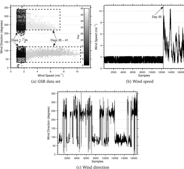
4.3.3 Grand-St-Bernard Data Set . . . 72
4.3.4 MNIST Data Stream . . . 72
4.3.5 Conclusion . . . 74
4.4 Anomaly Detection in a Non-Stationary Environment with KPCA . . . 75
4.4.1 Adaptive KPCA for Anomaly Detection . . . 75
4.4.2 Merging Eigenspaces in Kernel Space . . . 76
4.4.3 Splitting Eigenspaces in Kernel Space . . . 78
4.4.4 Cholesky Decomposition Incremental Update and Downdate . . . 80
4.4.5 Adaptive Scheme . . . 81
4.5 Evaluation - Kernel Eigenspace Splitting and Merging . . . 83
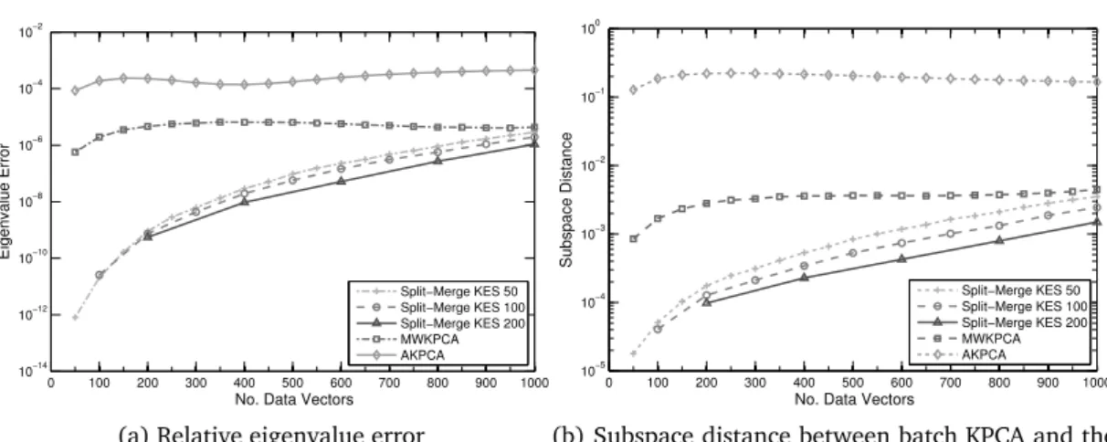
4.5.1 Accuracy Analysis of Incremental KES Algorithms . . . 83
4.5.2 Complexity Analysis . . . 87
4.5.3 Anomaly Detection Performance Metrics . . . 89
4.5.4 Data Sets . . . 90
4.5.5 Anomaly Detection Performance . . . 91
4.5.6 Impact of Imbalanced Distribution . . . 93
4.5.7 Adaptive Update . . . 93
4.5.8 Summary of Anomaly Detection Performance . . . 94
4.5.9 Conclusion . . . 95
4.6 Summary . . . 96
5 Anomaly Detection using Adaptive Parameter Selection 97 5.1 Background and Motivation . . . 98
5.2 Adaptive and Online Anomaly Rate Tracking . . . 101
5.2.1 Model Selection . . . 101
5.2.2 Effect ofν on the Model and Performance . . . 102
5.2.3 ν Identification in the One-Class Quarter-Sphere . . . 104
5.2.4 ν Identification with the RBF kernel . . . 105
5.2.5 ν APT andν RAPT . . . 107
5.2.6 Complexity Analysis . . . 111
5.3 Experimental Results and Evaluation . . . 111
5.3.1 Experimental Setup . . . 112
5.3.2 Accuracy of the Determination ofνwithνAPT andνRAPT . . . 114
5.3.3 Anomaly Rate Parameter Tracking . . . 115
5.4 Conclusion . . . 117
5.5 Summary . . . 118
6 Anomaly Detection in a Distributed Environment 119 6.1 Preliminaries and Problem Statement . . . 120
6.2 Distributed Minimum Volume Elliptical PCA . . . 121
6.2.1 Minimum Volume Elliptical PCA . . . 121
6.2.2 Distributed Minimum Volume Elliptical PCA . . . 123
6.2.3 Convergence . . . 125
6.3 Evaluation . . . 127
6.3.1 Network Topology . . . 127
6.3.2 Data Sets . . . 128
6.3.3 Performance Assessment . . . 129
6.3.4 MVE-PCA . . . 129
6.3.5 Distributed Anomaly Detection - Synthetic Data Set . . . 133
6.3.6 Distributed Anomaly Detection - Real-World Data Sets . . . 133
6.3.7 Complexity Analysis . . . 136
6.4 Conclusion . . . 138
6.5 Summary . . . 139
7 Conclusions and Future Work 140 7.1 Conclusions . . . 140
7.2 Summary of Research Achievements . . . 141
7.3 Future Research Directions . . . 143
List of Figures
1.1 The connections between the research in this thesis. . . 9
2.1 Schematic representation of the organization of the review of state-of-the-art. . . 13
2.2 Data set containing normal data and anomaly data. . . 14
2.3 Definitions of anomalies in data sets. . . 15
2.4 Representations of the effect of a non-stationary distribution. . . 24
2.5 Real-world non-stationary data set . . . 26
2.6 Arrival of data in a data stream. . . 27
2.7 Learning for incremental and batch algorithms. . . 28
2.8 Three different types of network. . . 38
3.1 The decision boundaries produced by the benchmark anomaly detection methods on a synthetic two dimensional data set. . . 53
3.2 The decision boundaries produced by the benchmark anomaly detection methods on a synthetic two dimensional data set. . . 54
3.3 The confusion matrix. . . 58
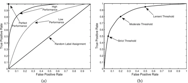
3.4 An illustration of the ROC space and the performance of an anomaly detector. . . 61
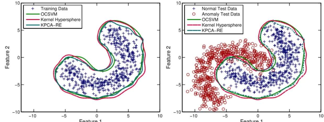
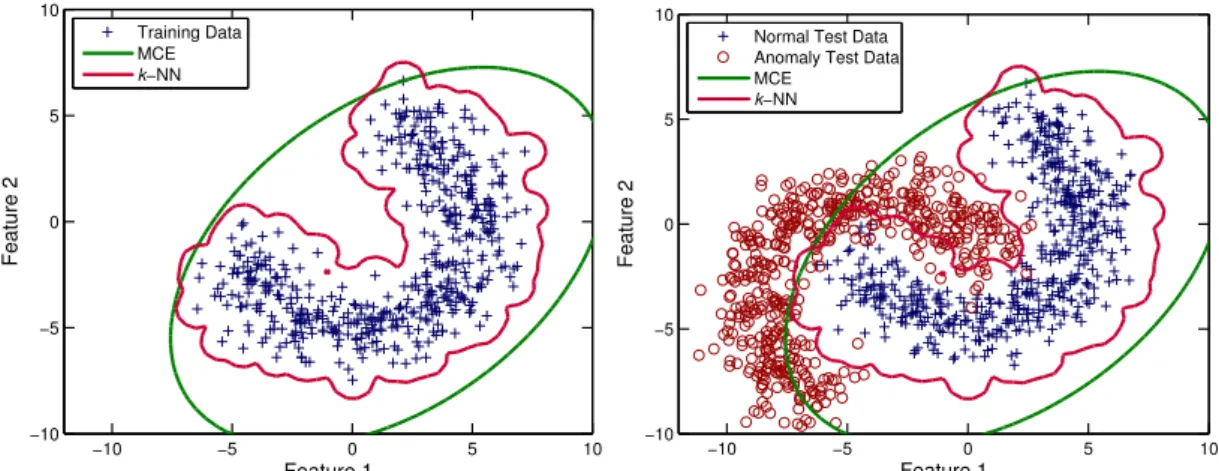
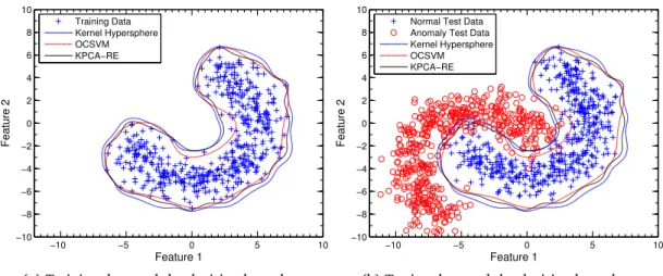
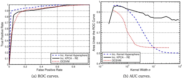
4.1 Decision boundary created by different anomaly detectors on the banana data set. . . 71
4.2 Performance of the incremental kernel hypersphere on a synthetic data set using the RBF kernel. . . 72
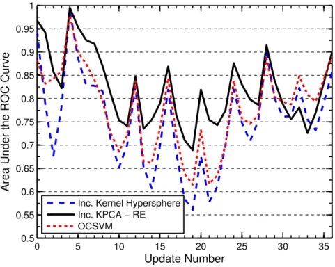
4.3 Performance of the incremental kernel hypersphere on the GSB data set using the RBF kernel. . . 73
4.4 AUC curve for the MNIST data stream using the RBF kernel. . . 74
4.5 Incremental update of a KES. . . 85
4.6 Incremental downdate of a KES. . . 85
4.7 Incremental downdate and update of a KES. . . 86
4.8 Incremental update and downdate with sine wave with noise data set. . 87
4.9 Timings of batch and incremental KPCA algorithms on the abalone data set. . . 90
4.10 Adaptive update of the KES applied to the MNIST data set. . . 95
5.1 The decision boundary for the linear and RBF kernel. . . 101
5.2 Impact of different values ofν on the decision boundary. . . 102
5.3 Effect of the value ofν on the F-measure. . . 103
5.4 Synthetic data set and the RBF kernel. . . 104
5.5 Synthetic data set and the linear kernel. . . 105
5.6 Wisconsin breast cancer data set for RBF kernel andσ= 0.6. . . 106
5.7 Pen digits data set for RBF kernel andσ = 2.0. . . 106
5.8 MNIST data set for RBF kernel andσ= 4.0. . . 107
5.9 Relationship betweenσand the separation distance for the synthetic data set. . . 108
5.10 Synthetic and Wisconsin breast cancer data set F-measure. and the σ parameter. . . 109
5.11 Pen digits and MNIST data set. F-measure and theσ parameter. . . 110
5.12 Details of concept drift, concept shift and reoccurring concepts. . . 114
5.13 Correlation between anomaly rate in the training set and the optimalν for the synthetic data set. . . 115
5.14 Correlation between anomaly rate in the training set and the optimalν for Wisconsin breast cancer and pen digits data set. . . 116
6.1 Visualization of the exchange of data between nodes. . . 124
6.2 Comparison of the PCs derived from PCA and MVE-PCA. . . 130
6.3 ROC curves for three of the data sets. . . 132
6.4 Snapshots of the first principal component derived for a synthetic training set evolving with time. . . 134
List of Tables
2.1 Summary of anomaly detection methods. . . 21
2.2 Summary of incremental anomaly detection methods. . . 33
2.3 Summary of model selection in anomaly detection methods. . . 36
2.4 Summary of distributed anomaly detection methods. . . 43
3.1 Real-world data sets. . . 56
3.2 Big O notation. . . 61
3.3 Complexity of the algorithms. . . 62
4.1 Complexity of techniques that operate in RKHS. . . 70
4.2 MNIST data stream. . . 73
4.3 Notation and variables. . . 77
4.4 Computational complexity of Split-Merge KES compared with other in-cremental KPCA techniques. . . 88
4.5 Description of data sets used to evaluate anomaly detection performance. 91 4.6 AUC scores for KPCA and alternative techniques for MNIST and PIE data sets. . . 92
4.7 AUC scores for KPCA and alternative techniques techniques for pen digits and abalone data sets. . . 93
4.8 AUC scores for KPCA and alternative techniques for varying anomaly rates. 94 4.9 AUC scores for Adaptive Split-Merge anomaly detection. . . 94
5.1 Adaptive learning. . . 117
6.1 Comparison of the complexities for the centralized and distributed schemes.127 6.2 Real-world data sets. . . 128
6.3 Comparison of centralized and local learning approaches. . . 131
6.4 Comparison of centralized and distributed learning approaches. . . 135
3.1 K-fold cross-validation method. . . 57
3.2 Grid search of the parameter space. . . 57
4.1 Pseudocode and summary of Split-Merge KES. . . 81
4.2 Pseudocode and summary of Adaptive Split-Merge KES. . . 83
5.1 Golden section search algorithm. . . 111
5.2 νadaptive parameter tracking (ν APT). . . 112
5.3 νrotated adaptive parameter tracking (ν RAPT). . . 113
6.1 Distributed MVE-PCA. . . 125
List of Abbreviations
ν APT ν adaptive parameter tracking
ν RAPT ν rotated adaptive parameter tracking
AKPCA adaptive KPCA
ADMM alternating direction method of multipliers ABOD angle-based outlier detection
ABOF angle-based outlier factor AUC area under ROC curve
ARMA auto-regressive moving average CPU central processing unit
CA consensus averaging DR detection rate FPN false negative rate FPR false positive rate GMM Gaussian mixture model
GSB Grand-St-Bernard
ICA independent component analysis
i.i.d independently and identically distributed IBRL Intel Berkeley Research Laboratory
KES kernel eigenspace
KHA kernel Hebbian algorithm
k-NN k-nearest neighbour
KMVCE kernel minimum volume covering ellipsoid
KPCA kernel principal component analysis KPC kernel principal components
KL Kullback-Leibler LOO leave-one-out
LOF local outlier factor
UCI Machine Learning Repository of UCI MCE mean centred ellipse
MDPN mean degree per node
MISE mean integrated squared error
MNIST Mixed National Institute of Standards and Technology
MV minimum volume
MVE minimum volume ellipse
MVE-PCA minimum volume elliptical PCA
MV-Set minimum volume set
MWKPCA moving window KPCA
NN nearest neighbour
NAMOS Networked Aquatic Microbial Observing System
NSE non-stationary environment
QS-SVM one-class quarter-sphere
OC-SVM one-class SVM
PA parallel analysis
PIE pose, illumination and expression PC principal component
PCA principal component analysis PDF probability density function RBF radial basis function
ROC receiver operating characteristic RLS recursive least squares
RS reduced set
RKHS reproducing kernel Hilbert space SPRT sequential probability ratio test
SV support vector
SVM support vector machine SVD singular value decomposition
SPE squared prediction error TNR true negative rate
TPR true positive rate
USPS US Postal Service handwritten digits recognition corpus WSN wireless sensor network
1
Introduction
Consider the problem of credit card fraud where the aim is to determine whether a submitted transaction is legitimate or fraudulent. Associated with the transaction are a number of measurements describing transaction amount, category, location, etc. These form a data instance which can be represented as a data vector. Using this information, is it possible to determine the legitimacy of the transaction?
Theoretically, there is an unknown function that is able to map the transaction into one of two classes, legitimate or fraudulent. The function is then used to classify the data instance as either legitimate or fraudulent. The problem is how to determine or estimate the function. Two approaches can be considered. The first approach examines the data instance and historical data in order to determine handcrafted rules or heuristics to represent the unknown function. For example, if the same transaction has been submitted previously, it might be presumed to be legitimate. A drawback of this approach is that it may lead to a proliferation of rules and exceptions which may lead to poor results. An alternative approach is to use a mathematical method to derive the unknown target function empirically from data. In other words, the aim is to learn the function from historical data. By looking for patterns in the data, it is possible to determine a function that will determine whether the transaction is legitimate or fraudulent. There are many different terms for learning from data. These include machine learning, pattern recognition and data mining. The methods developed under these terms can be considered facets of the same field as they largely overlap in scope. In this thesis, the term machine learning is generally used.
1.1
Background
One learning problem is to determine the function for data generated from an underly-ing process so that it is able to differentiate data generated from this process, from data generated from a different underlying process. The data generated from the underlying process are defined as the normal data and the data that are not from this process
are considered ananomaly. This problem is termedanomaly detection. An anomaly or outlier (these words are often used interchangeably) is defined as “an observation (or subset of observations) which appears to be inconsistent with the remainder of that set of data” [1]. Anomaly detection aims to identify data that do not conform to the patterns exhibited by the data set [2].
A machine learning approach to anomaly detection has distinct phases. The first stage is pre-processing of the data; the aim is to transform the data into a new space where the problem is easier to solve. The next stage is the training phase where the data set that is used to construct the model is identified. The following phase uses the training set in order to determine the model that represents the function that maps the labels onto the data. Once the model has been determined, the final stage is to use the model to assign labels to the testing data set. An important aspect of this is generalization, this refers to the model’s ability to classify examples that are not members of the training set.
Machine learning algorithms make assumptions about data that are used on them. An assumption is that the whole data set is available to one instance of the algorithm. Some domains in which machine learning is applied might not be able to make these assumptions. The following examples provide details of environments where these assumptions can not be made.
1.1.1 Application Examples
In this section some practical implementations are detailed where the research contribu-tions of this thesis can be applied. Three examples where anomaly detection has been implemented are fraud detection, monitoring in a wireless sensor network (WSN) and diagnosis and fault detection in medical data. Each domain involves different challenges, although they share common characteristics.
Financial Fraud Detection Anomaly detection has been used to detect financial fraud such as credit card fraud, insurance claim fraud and insider trader [2]. Plastic card fraud is defined as using plastic card payments, such as bank, debit, credit or store cards, to take money from a bank or charge money to the card without the card holder’s permission or prior knowledge. In 2011/2012, 4.7% of plastic card owners (around 2 million adults) were victims of plastic card fraud [3]. In an environment where behaviour is changing, there is a need to update the model. In addition, if credit card organizations are unable or unwilling to share and centralize the data set, learning must be performed on the distributed data set.
Monitoring in Wireless Sensor Networks Large scale monitoring applications such as smart city realisations [4], environmental monitoring [5, 6], industrial monitor-ing [7], internal buildmonitor-ing monitormonitor-ing [8] and surveillance [9, 10] provide valuable information for intelligent decision making and smart living. WSNs provide a plat-form for solving this monitoring challenge, which is low cost, easy to deploy, and require little or no maintenance during the lifetime of the network. Measurements
1.1. Background 3
collected by sensors form a time-ordered sequence of data. During the lifetime of data collection, the underlying phenomenon that is being measured may alter. This will cause a change in the distribution of the data which requires an update to the model. In addition, the data set in a WSN is distributed amongst a num-ber of nodes. Due to resources constraints it is not feasible to transmit the data to a centralized node. Therefore learning must be performed in the distributed manner.
Diagnosis and Fault Detection in the Medical Field Modern medical systems create large amounts of data and there is compelling evidence that applying machine learning methods to medical data can aid clinical decision making. Data instances are formed from two sources. The first is measurements made by both health care professionals and medical devices. The second source of data instances is medical images [11], for example the diagnosis of breast cancer through the detection of microcalcification in mammograms [12]. Data can have anomalies for a number of reasons, including abnormal patient condition, instrumentation and recording errors [2]. In an area such as this, it is necessary to have a high degree of accuracy and misclassification of data can have severe consequences. Patient records con-tain patient sensitive information and the exchange of information between sites can pose a privacy risk. In addition, if the data contain high resolution images, it may be infeasible to exchange the images between the sites.
From these applications, it is clear that there is a requirement to perform anomaly detection in two different environments. The first is a non-stationary environment where the data distribution alters. The second is an environment where data are distributed amongst a number of nodes in a network.
1.1.2 Non-Stationary Environment
Pattern recognition and machine learning techniques make an assumption that the training and testing data are drawn independently and identically distributed (i.i.d) from the same distribution. If this is not the case, then the model can be incorrectly constructed for the testing data. An incorrectly constructed model can cause a decision surface, which determines the label, to be incorrectly placed. Therefore data instances are misclassified and there is a decrease in performance. An environment in which data are generated from an underlying data distribution that is changing with time is termed anon-stationary environmentand the data generated are said to exhibitconcept drift[13].
In addition to selecting an appropriate technique to operate on a data set, the param-eters values for the technique must be chosen. The aim is to choose the paramparam-eters for the model that result in the best performance on the testing data set. Depending on the chosen technique, there can be a significant difference in the performance of two models of the same technique but with different parameters.Model Selectionis the process by which the parameters for a particular technique are chosen, and it can be performed in two ways; via heuristics and via parameter search. Heuristics are often
provided for algorithms where parameter values are specified that are expected to work well on a particular set of problems, whereas a parameter search involves identifying the parameters for a specific training set that will provide the best performance on unseen data. Training set selection is also an aspect of model selection in a non- stationary environment; to ensure that the model is optimal for the testing data it is important to include in the training set the examples that are drawn from the same distribution as the testing data.
1.1.3 Distributed Environment
Centralized learning, where the data set is available in its entirety to one classifier, is a well-studied area. However, if the data are distributed over more than one physical location, a different approach needs to be taken. For the centralized approach, this requires the communication of all data to a central node. This can be prohibitive if the data set is large. Robustness is also reduced as links close to the central node become critical. A local learning approach uses the data set in the local location to construct a classifier. This has the advantage that no communication between nodes is required. However, insufficient data might mean that the classifier is not representative of the whole data set, and different nodes will form different models. An alternative approach, distributed learning, aims to allow communication between nodes in order for nodes to construct a classifier that tends towards the centralized model. Nodes communicate summarized information about the local data set, with this information being used to construct a global classifier on each local node.
1.2
Problem Statement
The focus of this thesis is to investigate anomaly detection within two particular environ-ments. The first is where data is generated from a non-stationary data distribution. The second is where the whole data set is distributed across a number of nodes. In this thesis the two environments are addressed separately.
Pattern recognition and machine learning techniques make an assumption that the train-ing and testtrain-ing data are drawn i.i.d from the same distribution. If this is not the case then the model can be incorrectly constructed for the testing data. A solution to this problem is to reconstruct the model using the new training set, a batch reconstruction. However, model construction is often the most computationally complex task in the algorithm, and can be prohibitive if it has to be performed multiple times. Incrementally updating a model can reduce computational complexity by using the previous model and adding and removing data. This thesis proposes methods to reduce computational complexity of the update phase by using the previous model and incrementally adding and removing data. Two examples of classifiers are examined, the centred kernel hyper-sphere and kernel principal component analysis (KPCA).
An important aspect of model construction is the determination of the model parameters. Parameters provide a way to adapt model construction to a specific training set. If
1.3. Research Challenges 5
there is a change in the data distribution of the data, a model may require different parameters for the updated data set in order to obtain optimal performance. Model selection is the determination of the optimal parameters for a model. However, in unsupervised learning it is considered an open problem due to the lack of labels for the data instances in the training set. Methods for determining the optimal parameters either use heuristics to select the best model for the data or perform an exhaustive search across the entire parameter space. An open issue is parameter selection in the online environment where constraints mean that optimal model selection needs to occur efficiently and automatically in an unlabelled environment. This thesis addresses the issue of parameter selection in a non-stationary environment. A version of the one-class SVM (OC-SVM) is used and the variation of the anomaly rate in the training set is examined and how optimal parameters can be determined efficiently in an online environment where the training set is unlabelled and the anomaly rate varies.
Distributed learning aims to identify the data samples that are considered anomalous in the data set distributed across all the nodes in the network. These are termed the global anomalies. Often a hierarchical network architecture is assumed. This thesis proposes a distributed learning approach in which the underlying network has little infrastructure. Nodes operate without using information other than knowledge of its local neighbourhood and there does not exist unique identifiers for nodes which can be attached to messages [14]. Therefore, the network lacks the infrastructure to perform the routing of messages. In order to detect global anomalies on a local node, a classifier is constructed on a local node that, within some error bounds, is the classifier that would have been constructed had all the data been available to the local instance of the algorithm.
The two different environments, non-stationary and distributed, provide a significant challenge to anomaly detection. The ability of an anomaly detection algorithm to adapt models to a changing environment in an efficient manner will allow a model to perform optimally on testing data. Models that are able to adapt to changing concepts in the data are inherently more generic and will widen the applications into which they can be deployed. A distributed environment provides anomaly detection with a further problem in that all the data is not available to one instance of the machine learning algorithm. Algorithms that are able to learn in a distributed environment will further improve anomaly detection in application domains where data is distributed across a network of nodes.
1.3
Research Challenges
Pattern recognition and machine learning techniques make an assumption that the training and testing data are drawn i.i.d from the same distribution. If this is not the case then the model can be incorrectly constructed for the testing data. A solution to this problem is to reconstruct the model using the new training set. However, model construction is often the most computationally complex task in the algorithm, and can be prohibitive if it has to be performed multiple times.
deriving incremental forms of batch algorithms. An incremental algorithm takes the model previously constructed and then adds and/or removes additional data. This al-lows a model to be updated by adding data that represents the current data distribution and removing data that represents the previous data distribution. There are many ap-proaches to this technique. Some apap-proaches derive exact updates, whereas others make approximations of the model in order to allow the addition and removal of data. Approximations in the model can lead to inaccuracies, and a challenge of incremental techniques is to derive updates that are accurate. An incremental update should also be less computationally complex than performing a batch update. A further challenge is therefore deriving an incremental update that significantly reduces the cost in model generation while maintaining accuracy.
Most anomaly detection algorithms require the selection of model parameters. Perfor-mance can vary dramatically based on the values of the selected parameters. Many algorithms specify that parameter selection should be performed in order to construct the optimal model. For a labelled environment, cross-validation enables the determina-tion of parameters. This involves an exhaustive search over the parameter space that often occurs before the model is deployed. In a non-stationary environment, if the data distribution changes, the optimal parameters might also change. A key challenge is therefore determining the optimal parameters in a non-stationary environment. Multi-ple exhaustive searches over the parameter space are often infeasible. Automating the parameter search requires a measure that indicates the performance of a parameter value. However, in an environment where labels are not available, alternative measures of performance need to be determined. There have been attempts to perform automatic parameter selection, however, the techniques are only available for certain anomaly detection algorithms.
Machine learning algorithms assume that the whole data set is available to one instance of the learning algorithm. If data is distributed over a number of nodes which form a network, there are three choices. The first is to communicate all the data to one node, where a single instance of the machine learning algorithm can construct the anomaly detection model. This can be prohibitive in networks such as WSNs due to communica-tion cost and transmission errors. The second is to use the data on a local node to derive a local classifier. The drawback of this approach is that there might be insufficient data on the local node to represent the concepts of the whole data set. Therefore a major challenge is to derive the centralized model in a distributed environment without the communication of the whole data set to a centralized node. Summary information is communicated between nodes which usually requires significantly less communication than the whole data set. The algorithm attempts to derive or estimate the classifier that would have been constructed had all the data been available to one instance of the algorithm. The challenge lies in estimating the centralized classifier while minimizing communication between nodes.
1.4
Research Objectives
The research challenges listed in Section 1.3 indicate that anomaly detection in a non-stationary environment requires incremental updates to anomaly detection models
1.5. Scope 7
which are accurate and efficient. A further challenge of anomaly detection in a non-stationary environment is the determination of optimal parameters for a model. A final challenge is that of anomaly detection in a distributed environment where the network structure is flat. Therefore, the research objectives are to address challenges in the area of anomaly detection in the two environments of a non-stationary data set and a distributed environment.
Research Objective 1: To reduce computational resources used to adapt a model to a non-stationary environment by using an incremental update. The incremental update for two models are examined; the centred kernel hypersphere and KPCA. The method will allow data to be added and removed from a model with reduced computational complexity, however, the impact on performance terms of anomaly detection accuracy should be minimal.
Research Objective 2: To perform model adaptation so that the optimal hypothesis from the hypothesis set can be selected. The classifier algorithm used is the one-class quarter-sphere (QS-SVM) and the optimal parameter for a model is determined in an efficient manner by minimizing model construction. The perfor-mance on a non-stationary data set of the model constructed from the optimal parameter should exceed that of a model constructed with a statically selected parameter.
Research Objective 3: To perform anomaly detection in a distributed environment where a node only uses knowledge of its local neighbourhood and nodes do not have unique identifiers which can be attached to messages in order to perform message routing in the network. A PCA-like approach to anomaly detection is used as this is shown to exhibit excellent performance and can be derived in a dis-tributed form. The model constructed on each node should provide performance equal to that of the model derived from the whole data set.
1.5
Scope
The research conducted as part of this thesis is generic in context. The aim is to solve the problem of updating models in a non-stationary environment and in an environment where the data is distributed across a number of nodes in a network. An example application is a WSN; in this context there are resource constraints. Nodes have reduced computational capacity, in addition, the whole data set is distributed across a large number of nodes and due to transmission consuming a high proportion of the available energy, these must be limited. Therefore, there is a requirement to perform anomaly detection while reducing both computational and transmission cost.
Reducing computational and transmission cost can also be a goal in contexts other than a WSN. For example, if the size of the training data set increases significantly there is a requirement to reduce computational complexity. For many machine learning algorithms, the resources required for the construction of the model increases as a function of the size of the training data set. The computational cost can quickly exceed
the resources available to even the most powerful processor, and therefore there is a similar requirement to reduce the computational cost of the algorithm. A similar argument can be applied to the transmission of data. For a large training data set, it may be infeasible to communicate the large amount of data between nodes due to the amount of resources, such as bandwidth or time, required. Instead of the energy cost of transmission requiring a reduction, a large data set is the reason for the reduction. Therefore, it can be seen that fewer resources and an adequately sized training set (a WSN), and more resources and a large training set (a wired server infrastructure) both equate to the available resources not being sufficient to complete the task at hand. This requires methods to reduce the amount of resources required by an algorithm.
1.6
Contributions
To fulfil the objectives specified in Section 1.4, a summary of the main contributions are provided below. The connections between the research contributions is illustrated in Figure 1.1. More detailed presentations are provided in later chapters.
Contribution 1: An incremental anomaly detection scheme based on the centred kernel hypersphere is proposed. The algorithm is able to perform an exact incremental update and downdate to the model by tracking the centre and radius of the kernel hypersphere. The model is less computationally complex than other kernel-based anomaly detection techniques such as the OC-SVM or KPCA. Evaluations show that although the OC-SVM or KPCA outperform the algorithm, it remains competitive. Contribution 2: An incremental anomaly detection scheme based on KPCA is proposed. An incremental downdate to the kernel eigenspace (KES) of KPCA is proposed based on eigenspace splitting. This is coupled with an incremental update based on eigenspace merging to form the SplitMerge KES algorithm. Using the algorithm, data are able to be added to and removed from the KES. This offers reduced computational complexity when compared to a batch update. Using the recon-struction error and the KES, anomaly detection is performed. Evaluations show that the technique is more accurate with lower computational complexity than alternative state-of-the-art incremental KES update/downdate algorithms. In ad-dition, it is shown that KPCA and the reconstruction error is an excellent anomaly detection algorithm when compared with other state-of-the-art techniques. Contribution 3: A parameter selection algorithm for the QS-SVM is proposed. The
algorithm aims to determine the value of theν parameter, which represents the fraction of anomalies in the training set. It is shown that there is an optimal value ofν, and that this provides significantly improved performance. The optimal value is estimated in an efficient manner using a golden-section search of the parameter space. Evaluations on synthetic and real-world data show that the optimal value ofν can be determined.
Contribution 4: A distributed anomaly detection scheme, minimum volume elliptical PCA (MVE-PCA), based on a robust form of principal component analysis (PCA) is
1.7. Structure of the Thesis 9
Anomaly Detection
Non-Stationary
Environment Distributed Environment
Incremental Update Adaptive Parameter Selection Chapter 4 Incremental Centred Kernel Hypersphere Chapter 4 Split-Merge KES Chapter 5 One-Class Quartersphere ν Parameter Selection Chapter 6 Distributed Minimum Volume Elliptical PCA
Research
Figure 1.1: The connections between the research in this thesis.
proposed. The scheme uses the solution to a convex optimization problem which forms a minimum volume ellipse (MVE) around the data set. Slack variables allow some data to reside outside of the MVE. From the MVE, the principal components are derived from an eigen decomposition of the transformation matrix. Evaluation results show that MVE-PCA is a more robust anomaly detector when anomalies are present in the training set. MVE-PCA is derived in a distributed form using the alternating direction method of multipliers (ADMM). This enables local nodes to iterate towards the centralized solution by exchanging a matrix and a vector, rather than the whole training set. Evaluations on synthetic and real-world data show that the distributed form is able to iterate towards the centralized solution.
1.7
Structure of the Thesis
The thesis is organized into seven chapters. Brief summaries of each of the chapters are presented as follows.
Chapter 1 (Introduction)introduces the background knowledge to the field of anomaly detection using machine learning techniques. This chapter describes the research challenges, states core objectives of this thesis and lists the contributions to exist-ing research.
Chapter 2 (Related Works)identifies the main features of anomaly detection in non-stationary and distributed environments. Different approaches to anomaly detec-tion are discussed. An examinadetec-tion of the state-of-the-art of anomaly detecdetec-tion is performed in the two environments that are focused upon in this thesis. Anomaly detection is examined in a non-stationary environment where the distribution of the data evolves over time and there is a requirement to reconstruct the model. In
addition, a distributed environment is examined where the data are not available to one instance of the learning algorithm, but are distributed over a number of nodes that can communicate with each other.
Chapter 3 (Background and Research Methodology) discusses the approach towards
anomaly detection in non-stationary and distributed environments.
Chapter 4 (Incremental Learning) focuses on anomaly detection in a non-stationary environment. The anomaly detection model is incrementally updated by the addi-tion and removal of data instances. This allows the model to adapt to the evolving data distribution.
Chapter 5 (Adaptive Parameter Selection)details the adaptive selection of a parameter in a non-stationary environment. An algorithm is presented that is able to deter-mine the optimal parameter, whilst minimizing the number of models constructed. Chapter 6 (Distributed Learning) focuses on anomaly detection in a distributed envi-ronment where data are distributed amongst a number of nodes. The use of an anomaly detection model that is constructed from a convex optimization problem allows the problem to be recast as a distributed problem. Nodes are able to iterate towards the centralized solution through the exchange of a small number of data instances.
Chapter 7 (Conclusions and Future Work)concludes the thesis with a discussion of the extent to which the research objectives have been achieved. It also summarizes the contributions of the research and provides areas for future research.
1.8
Publications
The research work carried out during the course of this Ph.D has resulted in the follow-ing publications:
Journals
• C. O’Reilly, A. Gluhak, M. Imran, and S. Rajasegarar, “Anomaly detection in wire-less sensor networks in a non-stationary environment,”IEEE Communications Sur-veys & Tutorials, vol. 16, no. 3, pp. 1413–1432, 2014
• C. O’Reilly, A. Gluhak, and M. Imran, “Adaptive anomaly detection with kernel eigenspace splitting and merging,”IEEE Transactions on Knowledge and Data Engi-neering, vol. PP, no. 99, pp. 1–14, 2014
• C. O’Reilly, A. Gluhak, and M. Imran, “Distributed anomaly detection using mini-mum volume elliptical principal component analysis,”IEEE Transactions on Knowl-edge and Data Engineering (Under Review),
1.8. Publications 11
Peer Reviewed Conferences & Workshops
• C. O’Reilly, A. Gluhak, M. Imran, and S. Rajasegarar, “Online anomaly rate param-eter tracking for anomaly detection in wireless sensor networks,” inProceedings of 9th Annual IEEE Communication Society Conference on Sensor, Mesh and Ad Hoc Communication and Networks (SECON), Seoul, South Korea, Jun. 2012, pp. 191– 199
• C. O’Reilly, A. Gluhak, and M. Imran, “Online anomaly detection with an incremen-tal centred kernel hypersphere,” inProceedings of 23rd Annual IEEE International Workshop on Machine Learning for Signal Processing (MLSP), Southampton, UK, Sep. 2013, pp. 1–6
2
Related Works
This chapter provides a comprehensive review of anomaly detection in non-stationary and distributed environments. In Section 2.1 a definition of an anomaly is provided. Section 2.2 introduces the approach taken to anomaly detection. Section 2.3 reviews anomaly detection methods in an environment which is stationary and not distributed. In Section 2.4, anomaly detection in a non-stationary environment is examined. Sec-tions 2.5 and 2.6 present a detailed review of current state-of-the-art methods of anomaly detection in a non-stationary environment, this provides background to meth-ods relating to Objective 1 and Objective 2. Section 2.7 presents a review of anomaly detection in a distributed environment, this will provide background to methods relat-ing to Objective 3. Section 2.8 summarizes current challenges and identifies methods of improving the performance of anomaly detection algorithms in non- stationary and distributed environments. Figure 2.1 provides a visual representation of the structure of this chapter.
2.1
Definition of an Anomaly
The term anomaly is used to identify specific data instances in a data set. Two definitions of an anomaly in a data set are;
Hawkins [20] : “An outlier is an observation, which deviates so much from other obser-vations as to arouse suspicions that it was generated by a different mechanism.” Barnett [1] : “An observation (or subset of observations) which appears to be
inconsis-tent with the remainder of the data.”
The definitions illustrate how an anomaly is a data instance that significantly differs from other data instances in the data set. There is also reason to believe that an anomaly is the result of an underlying process that is different to the underlying process that generated the normal data instances. An illustration of normal and anomaly data instances in a
2.1. Definition of an Anomaly 13
Anomaly Detection – Background and Related Works
Distributed
Learning 2.7
Incremental
2.5
Model Selection
2.6
Non-Stationary 2.4
Medical
Sensor
Networks
Network
Monitoring
Image
Definition 2.1
Approach 2.2
Distributed
Learning 2.9.3
Incremental
2.9.1
Model Selection
2.9.2
Applications 2.8
Beyond State-of-the-Art 2.9
Probabilistic
2.3.1
Distance-Based
2.3.2
Subspace-Based
2.3.3
Domain-Based
2.3 4
Anomaly Detection Methods 2.3
Figure 2.1: Schematic representation of the organization of the review of state-of-the-art. Each box contains the section or subsection title and number.
simple two-dimensional synthetic data set is provided in Figure 2.2. The data instances occupy a main area, however, lying external to these areas are several data instances. These are considered to differ greatly from the normal data instances and therefore, according to the definition, these are considered to be anomalies in the data set. Anomalies in data have numerous causes and are usually specific to the application domain. For example, in the application domain of credit card fraud, the normal data will be the non-fraudulent transactions of the holder of the credit card. However, if a fraudulent transaction is made, this might have characteristics that differ significantly from the non-fraudulent transactions. Another cause of an anomaly is a data instance generated in error, termed a data fault. A data fault can be a data instance generated by a faulty device, such as a sensor, or a data fault can be a normal data instance that is corrupted or altered during storage. Data faults are measurements that are inconsistent with the nature of the phenomenon being observed [21] and identifying this type of error is important as they can cause data to be added to the data set that do not correspond to the underlying distribution.
Anomalies with different causes may have different characteristics, however, it is useful to categorize anomalies based on various properties. Properties include how much an
−1 −0.5 0 0.5 1 −1 −0.5 0 0.5 1
Feature 1
Feature 2
Normal AnomalyFigure 2.2: Data set containing normal data and anomaly data.
anomaly differs from normal data instances and the number of occurrences. Zhanget al.[22] classify anomalies based on the cause of the anomaly.
Type 1: Incidental absolute errors: A short-term extremely high anomalous measure-ment
Type 2: Clustered absolute errors: A continuous sequence ofType 1errors
Type 3: Random errors: Short-term observations not lying within the normal threshold of observations
Type 4: Long term errors: A continuous sequence ofType 3errors
Figure 2.3(a) displays the anomalies defined by Zhanget al.. At time period 20 a type 1 anomaly occurs as this data instance differs significantly from the normal data, but lies within the observation range. From time period 40 to 45 an extended burst of type 1 anomalies occurs. These are termed type 2 anomalies. At time period 60, a measurement occurs that significantly differs from the normal data and is outside the observation range. This is termed a type 3 anomaly. Finally, from time period 80 to 85 an extended burst of type 3 anomalies occurs. These are termed type 4 anomalies. Chandolaet al.[2] provide a different categorization of anomalies, Figure 2.3(b).
Point anomaly: An individual data instance that is considered anomalous with respect to the data set.
2.2. Approaches to Anomaly Detection 15 0 20 40 60 80 100 0 0.2 0.4 0.6 0.8 1 Time Sensor Measurement Type 1 Type 2 Type 3 Type 4 Normal Measurement Range
(a) Type 1, 2, 3 and 4 anomalies [22]
0 20 40 60 80 100 0 0.2 0.4 0.6 0.8 1 t1 t2 t3 t4 Time Sensor Measurement Contextual Anomaly Collective Anomalies Point Anomaly Normal Measurement Range
(b) Point, contextual and collective anomalies [2]
Figure 2.3: Definitions of anomalies in data sets.
Contextual anomaly: A data instance that is considered an anomaly in the current context. In a different context the same data instance might be considered normal. Collective anomalies: A collection of related anomalies.
A point anomaly occurs at time period 24 where the data instance is anomalous with respect to the entire data set. At time period 43 a contextual anomaly occurs which is anomalous at this time, but would not be considered anomalous had it occurred at time t1,t2,t3ort4. Finally, collective anomalies occur in the time period 54 – 71. Collective anomalies are a set of data instances that exhibit a pattern, however, they are anomalous with regard to the entire data set.
In this section, a definition for an anomaly in a data set has been provided. In the next section, the approach for detecting the anomalous data instances in data sets will be detailed.
2.2
Approaches to Anomaly Detection
Anomaly detection aims to identify data that do not conform to the patterns exhibited by the data set [2]. Several approaches can be taken to identify the anomalies in the data set. A supervised approach uses a labelled data set to construct the model. An unsupervised approach constructs the model with a training data set that does not have groundtruth labels.
The two-class classification problem constructs a model that is used to differentiate between two concepts (or classes). There is an unknown target functionf :X → Y, whereX is the input space andY is the output space. There is a data set of input-output examplesX = {xi, yi)}, wherexi is referred to as a data instance andyi is the label for this data instance. The collection forms thetrainingdata set. The hypothesis space
is the set of all hypotheses that might be returned by the learning algorithm. A learning algorithm selects a hypothesis, or function,g :X → Y that best approximatesf from a set of candidates from the hypothesis setH. It is clear that hypothess and model are synonymous; in this thesis the term model is generally used, except when the hypothesis space is considered.
However, there are serious shortcomings in applying two-class classification to anomaly detection. Anomaly detection assumes that normal data are well-sampled and anomalies are either non-existent or under-sampled in the training set. Therefore, although it is possible to construct a model for the normal data, it is not possible to construct an explicit model for the anomalies. Anomaly detection is usually performed within the framework of one-class classification [23], the problem of distinguishing one class from all other possibilities. One-class classification takes as inputX={xi)}, where there are no labels for the data instances. A one-class classification algorithm selects the function g:X → Y that maps a data instance in the testing data set onto a label of eithernormal
oranomaly. In anomaly detection, the aim is to identify the data instances that are not part of the normal data, the negative class. These are termed the anomaly data, the
positiveclass.
The class imbalance in the training set is due to several reasons. Anomalies may be costly to obtain or occur at a low frequency. In applications such as machine monitoring, the normal data will be generated through the normal operation of the machine, this data will be abundant. The anomaly data will be the result of the machine operating in an incorrect manner. There may be a small number of these data instances, however, they may be impossible to obtain without damaging the machine. In addition, it would be impossible to generate a well-sampled anomaly data set as this would involve breaking the machine in all possible ways. Therefore, it is difficult or impossible to obtain a well-sampled anomaly class [24]. In addition to solving the problem of an under-well-sampled anomaly class, the one-class classification framework allows the anomaly class to be drawn from multiple data distributions, as there is no attempt to model it. This is not true for the normal class which is assumed to be drawn independently and identically distributed (i.i.d) from the same data distribution. Anomalies may exist in the training data set and some algorithms are able to manage this, in others, the model is severely corrupted by presence of anomalies.
An anomaly detection algorithm will construct a model of normal data, also known as aclassifier. The classifier takes an input of a test data instance from the testing data set, and returns a label of normal or anomaly. In addition, some anomaly detection methods assign a score to a data instance, depending on the degree to which the data instance is considered an anomaly.
2.3
Anomaly Detection Methods
There are several taxonomies to categorize anomaly detection methods, in this thesis the taxonomy of Pimentelet al.[25] is used. Four categories are defined: probabilistic, distance-based, domain-based and subspace-based. In the following sections, the cate-gories are defined and a brief review of core methods and state-of-the-art approaches
2.3. Anomaly Detection Methods 17
is performed in order to provide a basis for the state-of-the-art review of methods for non-stationary and distributed anomaly detection.
2.3.1 Probabilistic Anomaly Detection
A probabilistic anomaly detection method aims to derive the generative probability density function (PDF) of the normal class. A threshold is then used to determine whether the test data instance has a high enough probability that it can be considered part of the normal distribution, or whether the data instance has such a low probability that it is considered unlikely to have been produced by the same underlying distribution as the normal data.
The estimation of the underlying density of the multivariate training data can be per-formed using parametric or non-parametric methods. A parametric approach makes assumptions about the distribution of the underlying population from which the sample was taken. The most common parametric assumption is that data are approximately normally distributed. Non-parametric tests do not rely on assumptions about the shape or parameters of the underlying population distribution.
One parametric approach is Gaussian mixture model (GMM)s, the assumption is that the data is generated from a weighted mixture of Gaussian distributions. The probabil-ity densprobabil-ity of the normal class is estimated using kernels, with the parameters being estimated using maximum likelihood methods such as expectation-maximization (EM). Songet al.[26] propose an EM algorithm for determining anomalies in data sets. The attributes of the data instances are partitioned into environmentaland indicator and two models are learnt using GMMs, one for the system behaviour and the other for the system environment. The two models are then used to determine the anomalies. Another non-parametric method is time-series methods such as auto-regressive moving average (ARMA). These techniques are used to predict the value the next data instance should take, and thus it can be determined whether it is normal or anomaly. Zhanget al.[27] propose an approach to construct a model using ARMA to create a stationary time series which is used to predict future values, actual measurements which lie outside the confidence interval are detected as outliers. A simplified version of the ARMA model was used to reduce computational cost. A drawback of the approach is that it operates on univariate data. To overcome this drawback, Galeano et al.[28] use a projection pursuit method to transform a multivariate time-series into a univariate one. A further approach uses adaptive Wiener filtering and ARMA [29] to anomalous network traffic. Kernel density estimators are a non-parametric technique, of which Parzen window [30] is one example, that uses kernel functions to estimate the density of the probability dis-tribution function. Kernel density estimators differ from histograms in that the density calculation is based on the interval placed around the observed value and not a prede-fined bin centre. A data instance that lies in a low probability area is classified as an anomaly. A nonparametric density estimate with a variable kernel to yield a robust local density estimation is proposed by Lateckiet al.[31]. A comparison between the local density of a test data instance and the local density of neighbours determines anomalies. Finket al.[32] perform anomaly detection using multivariate kernel density estimation
and a growing neural gas algorithm, an unsupervised artificial neural network. The method is shown not to be as sensitive to the high-dimensional data as other kernel den-sity estimation approaches. A comparison between kernel denden-sity methods and GMMs to estimate the joint PDF for the position-velocity of sea traffic [33] illustrated that kernel density methods had superior performance.
2.3.2 Distance-Based Anomaly Detection
Distance-based methods define the similarity of two data instances using a distance met-ric. There are two approaches; the distance of a data instance to other data instances and the relative density of the neighbourhood of a data instance. The concept of sim-ilar and dissimsim-ilar are defined through the measure. Distance-based methods include techniques such as nearest-neighbour and clustering.
Nearest-neighbour approaches assume that normal data instances will have neighbours which are close (in terms of the distance metric), while anomalies will be further from their neighbours. The Euclidean distance is often used as the distance metric. In k -nearest neighbour (k-NN) the distance to the kth nearest neighbour is used as the anomaly score, with a threshold determining if a data instance is normal or anoma-lous [34, 35]. Alternatives to this measure include a normalized distance [36], and a count of the number of neighbours who are not at a distance greater thandto the test data instance [37, 38].
A density-based approach, local outlier factor (LOF) [39], estimates the density of the neighbourhood of a data instance. The LOF score is the ratio of the average local density of theknearest neighbours of the data point and the local density of the data point itself. LOF has a computational complexity ofO(n2)wherenis the number of data instances in the training set. Many variations of LOF have been devised, for exampleGRIDLOF[40], reduces the computational cost of LOF by using a grid to prune non-outliers and then compute the LOF score for the remaining data.
As the number of dimensions of the data increases, the space occupied by the data be-comes increasingly sparse. In a sparse space, traditional concepts such as the Euclidean distance between points, and nearest neighbour, become irrelevant [41]. To overcome this drawback, angle-based outlier detection (ABOD) [42] replaces the distance mea-sure with the angles between pairs of data instances. The angle-based outlier factor is the variance of the angles between the difference vectors of the data instance to all pairs of data instances in the training set. Points within clusters will be surrounded by data instances and will have high variance, whereas data instances lying on a border will have lower variance. Outliers lying on one-size of the bulk of data will have the smallest variance. For each data instance, it is required to calculate the angle between all pairs of points, the computational complexity is thusO(n3). To overcome the com-putational complexity issue, FastABOD is proposed which uses angles between pairs of theknearest neighbours.
2.3. Anomaly Detection Methods 19
2.3.3 Subspace-Based Anomaly Detection
Subspace-based methods identify a lower dimensional subspace in which normal data can be differentiated from anomalous data. A test instance is then projected onto the subspace where the reconstruction error is defined as the distance between the test vector and the projection. Normal data will be easily modelled by the subspace and will therefore have a small reconstruction error. Anomalies will differ significantly from the subspace and will have a larger reconstruction error.
A lower dimensional space that occupies the maximal variance of the data set is derived by principal component analysis (PCA) [43]. PCA and the reconstruction error have been shown to perform well as an anomaly detection method [44–48]. An advantage of PCA is that high-dimensional data can be reduced to a more efficient lower-dimensional representation. Another application of PCA to anomaly detection [49] uses PCA to perform anomaly localization. The aim is to identify the sources that contribute most to the observed anomalies.
It is well-known that PCA is extremely fragile in the presence of anomalies in the training data set and even a small number of anomalies can significantly alter the subspace generated [50–52]. Various techniques have been proposed in order to overcome this issue. Multivariate trimming [53–55] aims to remove the outliers before deriving the principal component (PC)s from the clean training data set. Kwaket al.[56] use PCA with the L1-norm optimization, as opposed to the L2-norm, which is less sensitive to outliers. PCA with the L1-norm is shown to be more robust to anomaly data instances in the training set.
The use of kernel principal component analysis (KPCA) [57] as an anomaly detector was detailed by Hoffman [58]. By formulating PCA in terms of inner products, thekernel trick[59] allows its operation in a non-linear space where non-linear characteristics of the data are modelled. As with PCA, KPCA can be affected by anomalies in the training set. Xiaoet al. [60] derive KPCA in terms of the L1-norm and show that it is more robust to outliers in the training set. A drawback of the approach is that the eigen decomposition of the kernel matrix, which is Rn×n, is required. The computational
complexity of performing the eigen decomposition isO(n3).
2.3.4 Domain-Based Anomaly Detection
Domain-based anomaly detection methods define a boundary between the normal and anomalous data. The boundary defines thedomain of the normal data, with all data lying outside being considered as anomalies. Domain-based anomaly detection does not aim to determine the distribution of the data, as this is seen as unnecessary. According to Vapnik [61], “When solving a problem of interest, do not solve a more general problem as an intermediate step. Try to get the answer that you really need but not a more general one. According to this imperative: Do not estimate a density if you need to estimate a function.”
A simple technique to determine the boundary between the normal and anomaly data is to use a hypersphere or a hyperellipse to enclose the normal data. The distance metric
of Euclidean (hypersphere) and Mahalanobis (hyperellipse) can be used to determine the boundary and the distance of the data instances from the centre [35]. The boundary data instance can be determined using statistics such as chi-squared.
A drawback of using a hyperellipse to determine the boundary is that it is not robust to the presence of anomalies in the training set. To overcome this, Rousseeuwet al.[62] use the minimum volume ellipse (MVE) to provide robust estimates of the mean and covariance matrix. This technique was examined in detail by Jackson and Chen [63] and was shown to be more robust to outliers in the training data set when used in conjunction with the Mahalanobis distance. Multivariate trimming [53–55] aims to remove the outliers before deriving the PCs from the clean training data set.
The one-class SVM (OC-SVM) [64, 65] is a kernel method for anomaly detection that defines a boundary to separate normal and anomaly data. The hyperplane [65] sepa-rates the normal data from the origin with a maximal-margin hyperplane, allowing the anomalous data to lie between the hyperplane and the origin. The hypersphere [64] encloses normal data in a minimum-volume hypersphere, with the anomalies residing outside. The kernel trick [59] allows the projection of data into a space where data can be separated by a hyperplane or enclosed in a hypersphere. Theνparameter represents the upper-bound on the number of anomalies and lower-bound on the number of sup-port vector (SV)s [65]. In the case of the OC-SVM hypersphere, although slack variables allow some data instances to lie on the wrong side of the boundary, this does not neces-sarily create a minimum volume hypersphere. Pauwels and Ambekar [66] reformulate the cost function for the OC-SVM so that the centre of the sphere is a weighted me-dian of the support vectors, rather than the weighted mean of the support vectors. The OC-SVM has been the focus of much research, and several improvements have been proposed. Wu et al. [67] use the OC-SVM to create a maximal-margin hypersphere classifier that uses labels in the training set to create a hypersphere that separates the normal and anomaly data with a maximal margin. Liu et al.[68] use the anomalies in the data set to refine the boundary, showing that performance can be improved. A drawback of the OC-SVM is the requirement to solve a quadratic optimization problem, with computational complexityO(n3), to determine the boundary.
2.3.5 Overview of Anomaly Detection Methods
There are several methods that can be applied to detecting anomalies in data sets, with the foundations of the approaches lying in different mathematical fields. There are pros and cons to the methods, which must be taken into account when selecting a technique for the problem at hand. Some methods require a larger data set in order to construct an accurate model. Density-based methods are one example, [69], and in sparsely sampled data sets the performance might be poor. Probabilistic methods also require larger data sets to derive the PDF. Domain-based methods, such as the OC-SVM, are able to deal with smaller training sets [70]. A summary of the features and shortcomings of the methods reviewed is provided in Table 2.1.
This section has provided a general overview of the approaches taken to anomaly detec-tion. In the following sections, state-of-the-art is reviewed in the specific environments of non-stationary data sets and distributed data sets.
2.4. A Non-Stationary Environment 21
Method Features Shortcomings
Probabilistic [26–32]
Data set can be represented by minimal information. Statistically justifiable labels
with confidence intervals.
Requires larger data set. Some methods do not capture the relationship between
attributes. Distance-Based [34–
36, 39, 40, 42]
Noa prioriassumption on the data. Rely on the existence of a suitable distance
metric.
Distance metric becomes meaningless in high dimensional spaces. The
classification phase has high computational complexity. Subspace-Based [44–
49, 58, 60] Reduction in dimensionality of data.
Must ide