Boundary Bound Diffraction:
A combined Spectral and Bohmian Analysis
Jalal Tounli1, Aitor Alvarado2and Ángel S. Sanz3,*ID
1 2 3 4 5 6 7 8 9 10 11 12 13 14 15 16 17 18 19 20
21 22
DepartmentofOptics,FacultyofPhysicalSciences,UniversidadComplutensedeMadrid, Pza.Ciencias1,CiudadUniversitaria,28040Madrid,Spain;
1[email protected],2[email protected],3[email protected]
* Correspondence:[email protected];Tel.:+34-91-394-4673 ‡ Theseauthorscontributedequallytothiswork.
Abstract: The diffraction-like process displayed by a spatially localized matter wave is here analyzed
in a case where the free evolution is frustrated by the presence of hard-wall-type boundaries (beyond the initial localization region). The phenomenon is investigated in the context of a nonrelativistic, spinless particle with mass mconfined in a one-dimensional b ox, combining the
spectral decomposition of the initially localized wave function (treated as a coherent superposition of energy eigenfunctions) with a dynamical analysis based on the hydrodynamic or Bohmian formulation of quantum mechanics. Actually, such a decomposition has been used to devise a simple and efficient analytical algorithm that simplifies the computation of velocity fields (flows) and trajectories. As it is shown, the development of space-time patters inside the cavity depends on three key elements: the shape of the initial wave function, the mass of the particle considered, and the relative extension of the initial state with respect to the total length spanned by the cavity. From the spectral decomposition it is possible to identify how each one of these elements contribute to the localized matter wave and its evolution; the Bohmian analysis, on the other hand, reveals aspects connected to the diffraction dynamics and the subsequent appearance of interference traits, particularly recurrences and full revivals of the initial state, which constitute the source of the characteristic symmetries displayed by these patterns. It is also found that, because of the presence of confining boundaries, even in cases of increasingly large box lengths, no Fraunhofer-like diffraction features can be observed, as happens when the same wave evolves in free space. Although the analysis here is applied to matter waves, its methodology and conclusions are also applicable to confined modes of electromagnetic radiation (e.g., light propagating through optical fibers).
Keywords: diffraction; Moshinsky shutter; spectral analysis; Bohmian mechanics; interference;
quantum carpet; matter-wave optics
PACS: 03.65.Ca, 42.25.Hz, 67.10.Jn 23
1. Introduction 24
It is well known that matter waves spatially localized at a given time eventually undergo
25
delocalization when they are allowed to freely evolve. This behavior is exhibited, for example,
26
by trapped neutral atoms or condensates that are suddenly released [1,2]; once the atomic cloud is
27
released, it starts loosing localization as it spreads in time. An analogous behavior is also displayed by
28
matter wave crossing openings [3] or gratings [4–7]. In this case, the passage through the opening or
29
openings produces a number of transmitted (spatially localized) beams that, with time, undergo
30
delocalization by diffraction, giving rise to the appearance in the long-time regime to a spatial
31
redistribution of the probability — the so-called Frauhofer diffraction pattern. The latter scenario
32
is actually directly related to so-called diffraction in time phenomenon and the Moshinsky shutter
33
problem, introduced by Moshinsky in 1952 [8,9] to explain the appearance of transient terms in
34
dynamical descriptions of resonance scattering [10]. In this phenomenon, diffraction-like features
35
arise when a rather nonlocalized wave (e.g., a plane wave) is suddenly truncated (by the action of a
36
straight-edged shutter), thus producing a localized wave. The subsequent transverse evolution of this
37
wave is analogous to the evolution of a wave diffracted by a real opening. Diffraction in time has been
38
a subject of interest in the literature ever since [11–18], being first confirmed with the time-domain
39
analogous of single- and two-slit diffraction [19]. It is worth noting that, actually, this phenomenon is
40
analogous to considering the evolution of a wave under paraxial conditions, which allows to separate
41
the problem into the longitudinal (fast) propagation, characterized by a classical-like motion, and the
42
transverse propagation, describable in terms of a Schrödinger equation of reduced dimensionality
43
[20,21].
44
The delocalization displayed by an initially localized matter wave can be, however, spatially
45
limited by adding some extra boundaries, which gives rise to additional phenomena. Think, for
46
instance, of such a matter wave as in the Moshinsky problem, i.e., and extended wave entering a
47
cavity. The initial localization of the ingoing state, produced by the size of the input shutter, evolves
48
into a rather symmetric patter in space and time displaying, at some positions and times, recurrences
49
and even full revivals of the initially localized state [22,23]. Due to the similarity between these
50
patterns and usual carpets, they are calledquantum carpets[24], which may show fractal features under
51
certain conditions [25,26]. The emergence of such a pattern can be explained in terms of a complex
52
interference process involving a number of energy eigenstates of the confining cavity. Now, although
53
this is a bound effect, it is worth noting that an analogous situation also takes place in the continuum
54
when considering the transmission through a diffraction grating. In such a case, a repetitive pattern
55
arises by virtue of the so-called Talbot effect [27,28], used in optics, for instance, in lensless imaging
56
applications [29], but in matter-wave interferometry [30,31] to probe the wave behavior and related
57
properties of electrons [32], atoms [33] or large molecular systems [7,34]. Interestingly, in this case,
58
although there are no physical impenetrable walls constraining the evolution of the wave function, a
59
series of periodic non-physical interference-mediated walls arise as a consequence of the translational
60
invariance symmetry displayed by the initial state [35]. These walls are such that the quantum flux
61
confined within them remains the same all the way through (unless the translational symmetry is
62
spatially limited), generating patterns with recurrences and full revivals analogous to those observed
63
in the problem we are dealing with here.
64
If we focus on the propagation itself of the matter wave inside the cavity, this is an interesting diffusion-like problem where interference arises just because the complex nature of the probability amplitude or wave function, which is the quantity that diffuses throughout the available configuration space. In this regard, it is worth noting that, although Schrödinger’s equation is commonly regarded as a wave equation, formally speaking it has more in common with the heat-diffusion equation,1since both are parabolic partial differential equations [36]. That is, the evolution of matter waves and the propagation of heat both follow an equation of the kind
∂u ∂t −D∇
2u=0, (1)
where the distribution or field variableu(r,t)specifies the state of the system (i.e., the value of the
65
probability amplitude or the temperature, respectively) at any (allowed) positionrat a given timet. In
66
this equation, the diffusivity constantDplays a fundamental role, because it determines the diffusion
67
rate ofu. Now, while in the heat equationDis a real number without a specific predetermined value,
68
when dealing with quantum systems,Dis a pure imaginary constant with valueih¯/2m[37,38] (other
69
1 Of course, there is an important limitation in this analogy: while the diffusion equation arises from a conservation law,
authors [39] have considered alternative approaches whereDis real, although its modulus remains
70
the same). On the one hand, by virtue of the complex-valuedness ofDwe can observe interference
71
traits when dealing with quantum systems (which is not the case in heat transfer problems). On the
72
other hand, we find that, becauseDdepends on an external parameter, namely the mass associated
73
with the matter wave (in many-body problems there can be several of these constants, each one with a
74
different associated mass), the smaller the mass, the larger its diffusivity, which translates into a faster
75
spreading or delocalization rate.
76
The problem described by Eq. (1) is thus a typical boundary value problem, where a given (initial)
77
field functionu(x, 0), specified att=0, is constrained to vanish at the boundaries at any time, i.e.,
78
u(0,t) = u(L,t) = 0. With these boundary conditions, a particular set of solutions provided by
79
Eq. (1) is just the one formed by the energy eigenfunctions constrained to the cavity boundaries. From
80
these eigenfunctions localized solutions can be constructed, with their delocalization rate being a
81
function ofD, which in turn can also be understood in terms of the complex interference process
82
mentioned above as well as in terms of its associated flux. In this regard, the analysis results more
83
efficient when combining the use of the energy spectrum of the cavity, to analytically determine the
84
evolution of the system quantum state, with the numerically determined Bohmian trajectories, used to
85
follow the evolution of the system at a local level inside the box. As it will be shown in the problem
86
analyzed here, the first provides us with an efficient method to compute the governing velocity (flux)
87
fields (apart from other quantities of interest, such as the probability density), while the latter offers
88
an insightful picture on how and why the probability evolves in the way it does, explaining the
89
pattern formation characteristic of these systems. Besides its inherently fundamental interest to better
90
understand the processes of interference and recurrences in this kind of systems, as it will be seen
91
the analysis here conducted has an also intrinsic applied interest as a ground for the development of
92
efficient Bohmian-based numerical methodologies.
93
With such tools, in this work we investigate the problem of how the addition of extra boundaries
94
affects the evolution of an initially localized matter wave, i.e., how boundaries influence general
95
diffraction processes. To that end, we have considered the problem of the particle in a box, where the
96
system wave function att= 0 is a spatially localized state between two impenetrable walls, i.e., a
97
wave function with an everywhere vanishing amplitude except on a specific region between the box
98
boundaries, where it has finite values. This state describes a nonrelativistic, spinless particle of massm 99
in one dimension, with the cavity length beingLand the localization region having a widthw. This
100
can be the case, for example, of a neutron matter wave entering a waveguide [40] with rectangular
101
cross section at a relatively high speed (compared to other transversal dynamical scales) through a
102
shutter characterized by an aperture smaller than the size of the incoming wave and with a particular
103
transmission function (not necessarily homogeneous along the opening).
104
The pattern formation inside this type of cavities is well-known in the literature, so here we have
105
focused on three key aspects that rule the dynamical behavior of the system: the shape of the initial
106
localized state, the particle mass, and the relative extension of the cavity with respect to the size of
107
the localization region of the state. The first factor is related to the way how a shutter may transmit a
108
matter wave incident on it. From optics, we are used to homogeneous functions, although this may
109
not be the case if there are short-range interactions between the particles described by the matter wave
110
(e.g., electrons, neutrons, atoms, molecules, etc.) and the constituents of the material support where
111
the shutter is, which are often neglected, although they may have an important influence [5,41,42]. The
112
second factor, the mass of the particle, is important regarding the visualization of wave effects, since
113
larger masses should display classical-like features. This introduces the question of the classical limit
114
in a more natural way than the standard one typically based on the analyzing the behavior of energy
115
eigenfunctions under some particular limit. Finally, the third factor, the ratio between the size of the
116
cavity and the size of the region where the state is localized will render some light on the behavior
117
exhibited by the system when it gets gradually freer (by free it has to be understood the condition
118
when the confining boundaries go to infinity).
The work has been organized as follows. A general analysis of quantum diffraction in terms of
120
eigenfunctions of the infinite square well potential is presented in Section2, as well as the method to
121
compute the corresponding Bohmian trajectories in terms of such eigenfunctions. It is precisely by
122
virtue of this analysis, where we readily notice that the nonlinearity of the transport relation (Bohmian
123
equation of motion or guidance condition), that the mathematical superposition principle does not
124
have a direct physical counterpart. Accordingly, the evolution of the quantum system cannot be naively
125
described by appealing to independent waves (eigenfunctions), since the dynamics is governed by
126
the collective effect of all of them as a whole. This non-separability is a fundamental quantum trait
127
coming from the quantum phase, which translates into a non-crossing in the streamlines or trajectories
128
obtained in Bohmian mechanics. In Section3this analysis is applied to the study of the three different
129
elements that influence the evolution of the quantum system here considered: (1) the particular shape
130
of the system initial state, (2) its relative extension with respect to the size of the confining cavity, and
131
(3) the system mass. These analyses will make use of a combination of quantum carpets and associated
132
sets of Bohmian trajectories; the first will provide us with an overall perspective of the physics into
133
play, while the latter will show us the particularities of the probability flow. To conclude, a series of
134
remarks are summarized in Section4.
135
2. Theory 136
In the boundary value problem we are dealing with here, Eq. (1) takes the form of the
time-dependent Schrödinger equation,
ih¯ ∂ψ(x,t)
∂t =−
¯
h2
2m ∂2
∂x2ψ(x,t), (2)
whereψ(x,t)is constrained to the boundary conditionψ(−L/2,t) =ψ(L/2,t) =0 at any timetand Lis the total length of the box where the wave function is confined. The initial condition is specified by the localized state
ψ0(x) =
(
f(x), |x| ≤w/2
0, w/2<|x| ≤L/2 , (3)
withwbeing the effective size of the input shutter that allows the matter wave to enter the cavity.
137
2.1. Spectral analysis 138
Att=0, any general solutionψto (2) can be recast in terms of a coherent superposition of energy
eigenfunctions, as
ψ0(x) =
∑
αcαϕα(x). (4)
Since in one dimension theϕαare real functions, the coefficients are determined from the overlapping
integral
cα=
Z
ϕα(x)ψ0(x)dx, (5)
although the real-valuedness ofϕαdoes not ensure the real-valuedness ofcα, which also comes from 139
the value ofψ0— for instance, ifψ0(x)is a a traveling wave, e.g., a constant amplitude multiplied by a
140
phase factoreikx, then thec
αare complex-valued quantities. In the particular case of the infinite square 141
well here considered, the time-independent eigenfunctions read as
142
ϕeα(x) =
r 2
L cos(kαx), (6)
ϕoα(x) =
r 2
with
kα= πα
L . (8)
These solutions display, respectively, even (e) and odd (o) symmetry with respect to x = 0, i.e.,
143
φeα(−x) =φeα(−x)forα= 2n−1 andφoα(−x) =−φoα(x)forα= 2n, withn =1, 2, 3, . . . Physically, 144
these solutions indicate that only an integer number of half wavelengths can be accommodated
145
between the box boundaries, with the largest half-wavelength being equal to the total distance,L,
146
between them. The confining walls thus act in a way analogous to a space frequency (wavelength)
147
filter, removing any component that does not match such condition.
148
Following (4), any general initial condition can then be recast as
ψ0(x) =
∑
nce2n−1ϕe2n−1(x) +
∑
nco2nϕo2n(x). (9)
At any subsequent time, the wave function reads as
ψ(x,t) =
∑
αcαϕα(x)e
−iEαt/¯h=
∑
n
ce2n−1ϕe2n−1(x)e−iE2n−1t/¯h+
∑
nco2nϕo2n(x)e−iE2nt/¯h, (10)
since the time-evolution forϕαis given by
ϕα(x,t) =ϕα(x)e−iEαt/¯h, (11)
where
Eα = p2α
2m =
π2h¯2α2
2mL2 (12)
is the corresponding energy eigenvalue (withpα=hk¯ α). Accordingly, if the transmitted wave function 149
(initial condition) is described by (3), we find three possibilities:
150
i) If f(x)is an even function, only the cosine series contributes to (10).
151
ii) If f(x)is an odd function, only the sine series contributes to (10).
152
iii) Iff(x)has no definite parity (asymmetric function), a general combination of cosine and sine
153
functions contributes to (10).
154
In cases (i) and (ii) the parity or symmetry of the wave function at any subsequent time is fully
155
preserved. The time-dependent phases (11) only affect the amplitude of the real and imaginary parts
156
of the corresponding eigenfunctions, but not their parity. Hence, when the collective effect of all
157
the contributing eigenfunctions is taken into account, the parity of their total linear combination
158
is also preserved. The same holds for f(x) ∈ C. In this case, the function can be split up into its
159
real and imaginary components, which are then recast in terms of the corresponding eigenfunction
160
decompositions. Contrary to directly operating over the full complex function, this procedure allows
161
us to take advantage of the symmetry of each component separately to perform the analysis.
162
Without loss of generality, from now on we shall consider the case of even-symmetric wave
163
functions with respect tox =0 (mirror symmetry), like (3). The corresponding time-dependent wave
164
function reads as
165
ψ(x,t) =
r 2
L
∑
n c2n−1cos(k2n−1x)e−iE2n−1t/¯h
=
r 2
Le
−iE1t/¯h
∑
n
c2n−1cos(k2n−1x)e−iω2n−1,1t, (13)
with
ω2n−1,1 ≡
E2n−1−E1
¯
h =
2π2¯h
forn ≥2 (forn=1,ω1,1 =0). From a dynamical viewpoint, the preceding global time-dependent
phase factor in (13) can be neglected, as it is seen bellow with the aid of Bohmian mechanics. The behavior exhibited with time is ruled by the set of characteristic frequenciesω2n−1,1, which introduce
a series of related time-scales,
τ2n−1,1 = 2
π
ω2n−1,1
= mL
2
π¯h
1
(n−1)n. (15)
Whenever the evolution time equals an integer multiple of the largest of these periods, that is, the one for whichn=2,
τ3,1=
mL2
2πh¯, (16)
we observe a full recurrence of the wave function (leaving aside the aforementioned global phase factor), since
ω2n−1,1τ3,1= (n−1)nπ (17)
is always an even integer ofπ. From now on we shall refer toτ3,1as the systemrecurrence time, which
166
will be denoted byτr. This is auniversalquantity that does not depend on the initial shape of the wave
167
function or its widthw, but only on the total length Lspanned by the cavity and the system mass
168
m. Apart fromτr, there are other sub-multiples of this quantity for which fractional recurrences can
169
be observed, as will be seen in Sec.3. In the particular case of initial wave functions characterized
170
by non-differentiable boundaries, the evolution is characterized by a series of alternate regular and
171
fractal-like (at irrational fractions ofτr) replicas [25,26]. These systems present an additional symmetry
172
known as selfsimilarity.
173
Apart from the time symmetry implicit in the fractional (or even fractal) recurrences mentioned
174
above, the time-evolving wave function also displays (spatial) mirror symmetry (the symmetry of the
175
initial state is preserved at any subsequent time) and time-reversal symmetry with respect toτr. This
176
can easily be seen through the probability density arising from (13),
177
ρ(x,t) = 2 Ln
∑
,n0c2n−1c2n0−1cos(k2n−1x)cos(k2n0−1x)cos(ω2n−1,2n0−1t),
= 2
L
∑
n c2
ncos2(k2n−1x) +
2
L n
∑
,n0 n6=n0c2n−1c2n0−1cos(k2n−1x)cos(k2n0−1x)cos(ω2n−1,2n0−1t(18)),
where the bare sum of separate densities plus the sum of the coherence terms has been made more apparent in the second equality. In (18) also notice the presence of the frequency
ω2n−1,2n0−1= E2n−1−E2n 0−1
¯
h =
2π2h¯2 mL2
(2n−1)n−(2n0−1)n0
, (19)
which generalizes the previous expression (14) to any pair ofnandn0 components [in (14), we had
n0=1]. If we exchangexby−xin Eq. (18), we readily find that
ρ(−x,t) =ρ(x,t), (20)
which is satisfied at any timet. According to this symmetry, all what happens in one half of the space
178
inside the box has a mirror replica in the other half.
179
Regarding the time symmetry, consider two times symmetrically picked up around the recurrence time, i.e.,t1=τr/2−tandt2=τr/2+t. Evaluating (18) att1and then att2, we find
withτr/2 playing the role of a critical or inversion time. This means that the density evolves in time
180
developing a series of interference features untilt=τr/2; then, it undergoes aninvolution, passing
181
through all the previous stages until it eventuallyrecollapses, reaching a state equal to the departure
182
state (with respect to the probability density, since the wave function, as seen above, accumulates a
183
global phase factor that makes it to be exactly the same we had at the beginning). To some extent the
184
situation is analogous to a closed universe (in terms of density rather than shape), where after reaching
185
maximum expansion, it collapses again. This behavior is independent of the shape of the initial state,
186
the system mass, or the extension of the confining box; in all cases an expansion (diffraction) and
187
recollapse of the system is expected (unless dissipation and/or decoherence are somehow present).
188
2.2. Bohmian analysis 189
The above spectral analysis allows us to understand the evolution of the matter wave inside the cavity by means of a complex interference process among different energy eigenfunctions. Instead of appealing to the energy representation, the same process can also be understood in the configuration representation, where the spatial interference observed (see Sec.3) is usually explained in terms of semi-classical argumentations based on the computation of classical orbits [43]. In this regard, Bohmian mechanics provides us with an alternative and complementary analysis tool based on locally monitoring the quantum flux with the aid of trajectories. This is possible by means of the nonlinear (polar) transformation
ψ(r,t) =ρ1/2(r,t)eiS(r,t)/¯h, (22)
which recast a complex-valued field (ψ) in terms of two real-valued fields, namely the probability 190
density, ρ, and the (wave function) phase, S. After substitution of (22) into the time-dependent 191
Schrödinger equation, two (real-valued) coupled partial differential equations arise,
192
∂ρ
∂t + ∇ ·J=0, (23)
∂S ∂t +
(∇S)2
2m +V+Q=0, (24)
withJ=ρ∇S/mbeing the usual probability current or quantum flux [44],
J=D(ψ∇ψ∗−ψ∗∇ψ). (25)
Equation (23) is the well-known continuity equation for the conservation of the probability, while (24), more interesting from a dynamical viewpoint, is the quantum Hamilton-Jacobi equation governing the particle motion under the action of a total effective potential:Veff=V+Q. The last term in the
left-hand side of (24),
Q=−h¯ 2
2m ∇2
ρ1/2
ρ1/2 , (26)
is the so-calledquantum potential, which depends on the system quantum state through the density
193
field.
194
mechanics in a natural fashion: particle trajectories are defined as the solutions of an equation of motion that admits different functional (convenient) functional forms,
˙
r= ∇S
m =
J ρ =
¯
h m Im
n
ψ−1∇ψ
o
= 1
m Re
pψˆ
ψ
. (27)
Here, ˆp = −i¯h∇is the usual momentum operator in the configuration representation. Notice that
195
v=r˙specifies a velocity field predetermined at each time by the value of the system wave function
196
ψ(through its phaseSor, equivalently, the fluxJ). This is particularly interesting att=0, since the 197
initial momentum is predetermined by the initial wave function, ψ0. This means that trajectories
198
(or, equivalently, quantum fluxes) must evolve in time following a given prescription, this being a
199
dynamical manifestation of the so-calledquantum coherence. Notice here the difference with respect to
200
point-like classical mechanical systems, with their initial momenta being independent of their initial
201
positions. In this sense, although both quantum and classical systems evolve under a similar equation,
202
namely a Hamilton-Jacobi equation, they cannot be directly compared because their dynamics are very
203
different. In the quantum (Bohmian) case, dynamics take place in configuration space, thus only being
204
dependent on coordinates [momenta are fixed at each point by the phase field, as it can be inferred
205
from Eq. (27)], while classical dynamics develop in phase space, where coordinates and momenta are
206
both independent variables.
207
Taking into account the explicit functional form of the wave function (13), the equation of motion
208
(27) for a general superposition of energy eigenfunctions takes the form
209
˙
x= 1
m
∑α,α0|cα||cα0|sin(kαx)cos(kα0x)sin(ωα,α0t+δα,α0)
∑α,α0|cα||cα0|cos(kαx)cos(kα0x)cos(ωα,α0t+δα,α0)
. (28)
In this equation, the coefficients preceding each eigenfunction have been recast in polar form,
cα=|cα|e
iδα, (29)
assuming that they may also introduce a complex phase factor. This explains the phase shiftsδα,α0 = 210
δα−δα0 that appear in both the numerator and the denominator of this equation. In our particular 211
case, though, thecαcoefficients are real, for whichδα=0, and therefore Eq. (28) acquires the simpler 212
functional form
213
˙
x= 1
m
∑α,α0cαcα0sin(kαx)cos(kα0x)sin(ωα,α0t)
∑α,α0cαcα0cos(kαx)cos(kα0x)cos(ωα,α0t)
. (30)
Because the velocity field (30) satisfies exactly the same symmetry conditions displayed byψ0,
214
it is expected that the trajectories will also manifest this kind of overall feature. However, it is also
215
possible to go the other way around and extract valuable information about the topology displayed by
216
the trajectories and, from it, about the dynamical behavior of the system. For example, the fact that
217
the solution trajectories obtained from (30) cannot cross the same space point at the same time [45]
218
implies that the dynamical behavior of the system can be split up into different domains. Specifically,
219
in the cases considered here the mirror symmetry with respect tox =0 translates into two separate
220
dynamical regions, with the trajectories from one domain never penetrating the other one, and vice
221
versa. This can easily be inferred from the fact thatv(x =0) =0 at any time, which means that the
222
quantum flux splits up into two separate fluxes, each one confined in one half of the box.
223
3. Numerical simulations 224
Diffraction is typically associated with functions or states characterized by well-defined edges,
225
even if this implies their non-differentiability on some particular space points. This is an interesting
226
aspect to be analyzed, for such edges strongly determine not only the speed or rate of the system
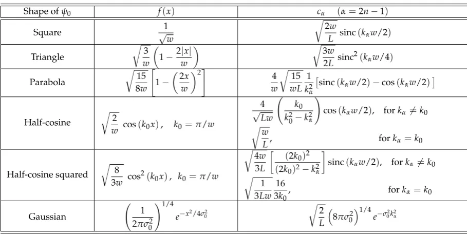
Table 1. Different functional shapes considered in this work for the (simulated) diffracted wave functionψ0and their corresponding Fourier components. The width of the Gaussian function,σ0= w/2π, has been chosen so that, in first approximation, it equals the squared half-cosine function
(moreover, with this value, the corresponding probability density has decreased to about 4% at
|x|=w/2). These wave functions are displayed in Fig.1(a).
Shape ofψ0 f(x) cα (α=2n−1)
Square √1
w
r
2w
L sinc(kαw/2)
Triangle
r
3
w
1−2|x|
w
r
3w
2L sinc 2(k
αw/4)
Parabola r 15 8w " 1− 2x w 2# 4 w r 15 wL 1 k2 α
sinc(kαw/2)−cos(kαw/2)
Half-cosine
r
2
w cos(k0x), k0=π/w
4
√
Lw k0 k2
0−k2α
!
cos(kαw/2), forkα6=k0
r
w
L, forkα=k0
Half-cosine squared
r
8 3w cos
2(k
0x), k0=π/w
r
4w
3L
(2k0)2 (2k0)2−k2
α
sinc(kαw/2), forkα6=k0
r
1 3Lw
16 3k0
, forkα=k0
Gaussian 1
2πσ02
!1/4
e−x2/4σ02
r
2
L
8πσ02
1/4
e−σ02k2α
diffusion inside the box, but also the type of recurrences that can be expected, which determines in the
228
last instance the transport properties of the box if it simulates, for instance, an optical fiber or the depth
229
of a slit to diffract matter waves (e.g., electrons, neutrons or atoms). Physically, this initial shape can be
230
related to the transmission function associated with the shutter, which does not necessarily has to be a
231
flat function all over its extension. On the contrary, it can be given in terms of a modulation function,
232
as happens when we insert optical filters for light or, in the case of matter waves, specified by the effect
233
of the potential mediating the interaction between the diffracted particle and the constituents of the
234
aperture. Analogously, as can be noticed through the functional form displayed by the time-dependent
235
wave function (13) and its recurrence time (15) [or its frequency (14)], the system massmas well as the
236
box lengthL(in relation to the dimension of the shutter or, equivalently, the space region where the
237
initial wave function is nonzero) are also going to play an important role in the subsequent evolution
238
of the wave and the type of interference features that it will develop with time. Below, the effects
239
of these three aspects on the system diffusion are going to be discussed with the aid of a series of
240
numerical simulations based on the analytical forms (18) for the probability densities, and (30) for the
241
velocity field and, by integration, the corresponding Bohmian trajectories.
242
To better understand the effects of these influential aspects and particulary to acquire a more quantitative idea of them, in the analysis we are going to consider some quantities of interest. One of them is theoverlapping probability, here defined as the overlap between the exact wave function,Ψ(x,t), and its associated series truncated at theNth term,ΨN(x,t), i.e.,
PN=
Z
Ψ∗
N(x,t)Ψ(x,t)dx= N
∑
n=1c22n−1. (31)
This quantity provides us with a direct measure of the convergence of the series and, therefore, how the above parameters influence the superposition and the subsequent interference traits developed along time. Another two quantities of interest are therelative weight c2
superposition as a function ofn, just to get an ide on the relevance of each contributing eigenfunction, and theexpectation value of the energyforΨN(x,t),
hHiN = ∑ N
n=1|c2n−1|2E2n−1
PN
, (32)
which is also a measure of convergence in terms of the energy added by each component to the
243
superposition.
244
3.1. Influence of the shape: matter-wave diffraction 245
First we are going to analyze the spreading or diffusion and subsequent interference and
246
recurrences in the position (configuration) space of a series of diffracted wavesψ0, an analysis that
247
emphasizes the relationship between such traits or phenomena and the relative curvature of the
248
diffracted function. We have chosen a series of functional forms f(x)for the initially localized wave
249
packet (see Table1) in a range that covers various intermediate functions, from the square function to
250
the Gaussian wave packet [see Fig.1(a)]. The square function constitutes a paradigm of transmission
251
function in both optics and quantum mechanics, although more realistic in the first case than in the
252
latter due to the faster propagation of light with respect to usual matter waves. The Gaussian function,
253
in many cases of physical interest, has a more convenient computationally functional form, apart from
254
being more realistic when short-range interactions with the opening boundaries are non-negligible.
255
As intermediate cases we have chosen a triangle, a parabola, a half-cosine and a half-cosine squared,
256
which present different degrees of differentiability and curvature. All these intermediate cases have
257
been chosen in such a way that they vanish atx=±w/2. As for the Gaussian function, its width has
258
been chosen in a way that, in first approximation, its functional form equals that of the half-cosine
259
squared, as can be seen in Fig.1(a) by means of the overlap of both functions for|x|.1/3. As can
260
be seen in the figure, the triangular function is quite close to these two functions, while the parabola
261
and half-cosine functions are closer between themselves. The decomposition of all these functions in
262
terms of energy eigenfunctions of the infinite square well potential can be seen in Table1in terms
263
of the genericαth coefficient, withα =2n−1. All the initial ansätze considered in Table1share a 264
general common feature worth mentioning, as can be noticed in their eigenfunction decomposition:
265
Ψ0does not depend on the system mass (m), but on the ratiow/L. However, despite this fact, the
266
dynamics displayed byΨ0is strongly dependent on the mass, since it appears in a key dynamical
267
element, namely the frequencies (14) and (19). According to the expressions for these frequencies,
268
the larger the mass, the lower the frequency (energy). These facts are related to the time-reverse and
269
mirror symmetries above discussed. Large masses and/or box lengths will imply longer recurrence
270
times, i.e., slower dynamics, as will be seen in more detail in Sec.3.2.
271
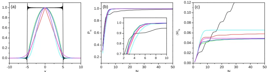
Let us now discuss in more detail some properties of the six wave functions. In Fig.1(a) we
272
observe a reconstruction of all the functions considered. A total of 500 eigenfunctions has been
273
considered in each case. As it can be seen (and is well known), the shape of each function is well
274
converged, except the square wave function due to the discontinuity atx=±w/2. This mismatch is
275
produced by the well-known Wilbraham-Gibbs phenomenon [46–48], which, in the context of Fourier
276
analysis, states that a Fourier series will display a finite increase or decrease of the value of the sampled
277
function at those points where the function has a discontinuity, independently of how many Fourier
278
components are considered in the series. Strictly speaking, although we are not performing Fourier
279
analysis, the decomposition of the function in terms of a basis set associated with a certain potential
280
function (an infinite square potential) is analogous. As a consequence, although the sum of components
281
approaches very slowly the normalization to unity, as seen in Fig.1(b), the expectation value of the
282
Hamiltonian is unbound, as shown in Fig.1(c). This is connected to fractal like features in the evolution
283
of the square function [25] each time that one looks at a time that is an irrational submultiple ofτr. This
284
behavior quickly disappears as the discontinuity at±w/2 also disappears, as can be seen in the other
285
cases shown in Figs.1(b) and (c). In Fig.1(b) the inset shows howPNapproaches the unity with a very
-10 -5 0 5 10 0.0
0.2 0.4 0.6 0.8
1.0 (a)
ψ0
(x
)
/
ψ0
(0
)
x
0 10 20 30 40 50
0.2 0.4 0.6 0.8
1.0 (b)
PN
N
0 10 20 30 40 50
0.00 0.02 0.04 0.06 0.08 0.10 0.12
〈
H
〉N
N
(c)
2 4 6 8 10
0.7 0.8 0.9 1.0
Figure 1. (a) Reconstruction of the six wave functions described in Table1with a total ofN =500 eigenfunctions each: square (black), triangle (red), parabola (green), half cosine (blue), half-cosine squared (cyan), and Gaussian (magenta). For a better comparison, all wave functions have been normalized to their value atx=0 (Ψ0(0)). In all cases:L=50,w=10, and ¯h=m=1. (b) Probability PN(31) as a function of the numberNof contributing eigenfunctions. For visual clarity, an enlargement ofPNfor lowNis shown in the inset. (c) Expectation value of the Hamiltonian (32) as a function of the numberNof eigenfunctions.
few eigenfunctions for all functions; in Fig.1(c) it is shown that, in spite of the nondifferentiability at
287
±w/2 for the triangle, the parabola and the half cosine, the expectation value of their energies remain
288
bound. In this regard, because of the nondifferentiability also atx=0, the convergence of the energy
289
for the triangle function is relatively slower than the other cases, since the number of contributing
290
eigenfunctions is larger.
291
So far we have commented on properties related to the construction of wave functions with
292
different initial shapes, which physically describe ways in which a shutter operates on an incoming
293
wave larger than its opening (e.g., a plane wave acted by a collimating slit). Let us now focus on the
294
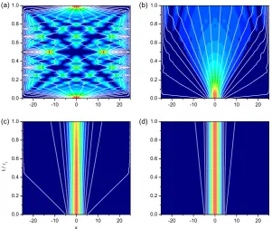
subsequent time-evolution of such waves. To that end a series of contourplots with the corresponding
295
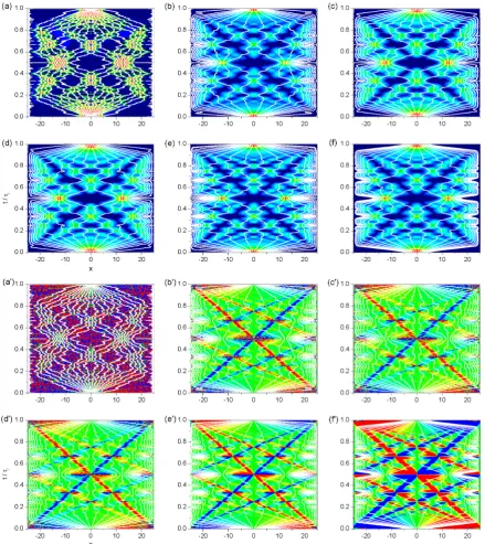
Bohmian trajectories have been represented in Fig.2for each case considered in Table1. The six
296
top panels represent the time-evolution (vertical axis; normalized to the recurrence timeτr) of the
297
corresponding probability densities, while the six bottom panels (labeled with a prime) describe the
298
evolution of the associated velocity fields. In both cases, and for each function, a set of 20 Bohmian
299
trajectories (white solid lines) is also shown, with the initial conditions evenly distributed along the
300
opening (or a bit further away for the Gaussian wave function, just to also sample the dynamics of
301
its “wings”). Perhaps such a distribution can be considered as misleading, since it is not a bona fide
302
representation or mapping of the evolution of the probability densityρ(x,t). However, the purpose 303
here is not to illustrate this behavior, which can be found elsewhere (see, for instance, [49] for diffraction
304
and interference in the open), but to get a glimpse on the features characterizing diffraction under
305
confinement conditions, which are more prominent for marginal trajectories than from those associated
306
with large values of the probability density.
307
By inspecting the behavior of the probability density, the first we notice is the presence of the two
308
kind of symmetries mentioned earlier. The space mirror symmetry displayed by the probability is
309
very apparent for the whole evolution of the wave function, fromt=0 tot=τr =397.9, although
310
the set of Bohmian trajectories reveals the specificities of the dynamics, that is, there is a fast motion
311
from some maxima to others, while avoiding those regions whereρis negligible. This is particularly 312
relevant near the boundaries of the box: although initially the trajectories spread very fast towards the
313
boundaries, after reaching them they start undergoing a series of bounces in order to avoid staying
314
close. Nonetheless, except in the case of the square function, where trajectories display fractal features
315
[26] and close to the borders they undergo very fast oscillations, in the other five cases the border
316
trajectories are relatively well-behaved, particularly in the Gaussian case. Besides, the trajectories
317
also make apparent that the system, for practical purposes, behaves as composed of two independent
Figure 2. Contour-plots showing the quantum carpets displayed by the six wave functions described in Table1along their evolution: (a) square, (b) triangle, (c) parabola, (d) cosine, (e) cosine square, and (f) Gaussian. The six upper panels represent the probability density, while the six lower panels (labeled with primes) refer to the corresponding velocity fields. Sets of quantum trajectories have been superimposed in order to illustrate the dynamical evolution of the flux in each case. In all cases:
halves, since the flux dynamics forx < 0 does not mix with that forx > 0, and vice versa. This
319
dynamical behavior is well understood if we look at the carpets corresponding to the velocity field
320
(bottom panels), characterized by the property of mirror antisymmetry, i.e.,v(−x,t) =−v(x,t). The
321
pronounced regions where the velocity field has large values are characterized by sudden and also
322
large values of the modulus of its first derivative, which provokes a fast dispersion of the trajectories.
323
On the other hand, the trajectories tend to accumulate in the regions where the first derivative of the
324
velocity field is relatively small and smooth.
325
When we examine the probability and velocity carpets along time, the second symmetry, namely
326
the time-reversal symmetry, immediately becomes apparent. After a very fast initial boost, the wave
327
function starts undergoing different recurrences by interference after having interacted with the box
328
boundaries, which generate the specific pattern of the carpet. Now, interestingly, att=τr/2, there is a
329
neat recollapse of the wave function, which gathers two features: the probability density is split up in
330
the form of a coherent superposition of two identical images of the initial density, each one centered
331
just at the center of each half of the box. If we look at the velocity carpets, what happens is that the
332
flux is eventually confined within these two localized regions att=τr/2, that is, the trajectories are
333
constrained to these two regions, like if there where two openings precisely at such positions. From
334
this time on, the behavior of the system reverts until we observe a full recollapse of the wave to its
335
initial state (neglecting the global phase factor accumulated with time, which is dynamically irrelevant,
336
as it was pointed out in Sec.2).
337
3.2. Influence of the mass: from geometric shadows to wave features 338
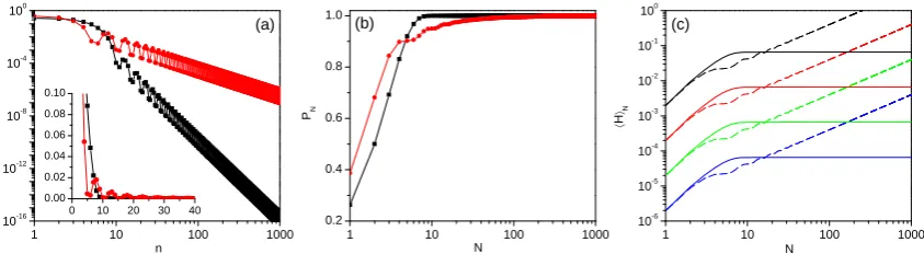
As can be seen in Table1, the system mass has no influence on the superposition itself. In
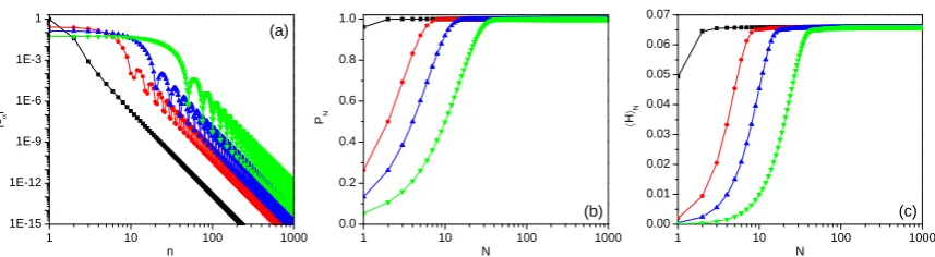
Figs.3(a) and (b) the weights|cα|2and the probabilityPNare shown for the square and half-cosine
squared wave functions. We have chosen here these two particular functions, because they both are nonzero only within the interval|x| ≤ x/2, with the particularities that the former is an example of non-differentiable function and the latter is close in behavior to the Gaussian. Since the initial spectral decomposition of the wave function does not depend on the system mass, the plots in these figures (for each function) are the same for the four masses considered in this section:m=1,m=10,
m= 100 andm= 1000. Figure3(a) allows us to observe the oscillatory behavior of the weighting
coefficients in both cases, which explains the also oscillatory behavior ofPNor the stepped structure of
hHˆiNthat we already saw in the previous section. Interestingly here, when comparing the square and the half-cosine squared functions, we notice that while the contribution of the eigenfunctions to the superposition (measured through|cα|2) decreases slowly withnfor the former, the decrease is very
fast for the latter (the same has also been observed for the other wave functions). For example, while about 10 eigenfunctions have a weight above 10−4for the half-cosine squared function, there are about 100 eigenfunctions in the case of the square function, which explains whyhHˆiNdisplays very clear steps in the latter case, while the same cannot be seen for the former [see Fig.1(c)]. The linear scale in the inset makes more apparent how, while the|cα|2coefficients are negligible beyondn=10 for the
half-cosine squared function, the same does not happen for the square function. The manifestation of this fact can be readily seen in Fig.3(b):PNis already about 1 forn≈10 for the half-cosine squared function, while for the square function it converges very slowly to 1. Furthermore, from a simple least square fitting, we have observed that the|cα|2decay asn−2for the square function and asn−6
for the half-cosine squared, which has interesting implications and an explanation for the unbound increase of the expectation value of the energy in the case of the square function. As seen in Sec.2, the eigenenergies increase withnapproximately liken2. So, if we compute the expectation value of the energy, we will have something like
hHˆi∝
∑
n
1 10 100 1000 0.2
0.4 0.6 0.8 1.0
1 10 100 1000
10-16
10-12
10-8
10-4
100
0 10 20 30 40
0.00 0.02 0.04 0.06 0.08 0.10
1 10 100 1000
10-6
10-5
10-4
10-3
10-2
10-1
100
(b)
PN
N
|cα
|
2
n
(a) (c)
〈
H
〉N
N
Figure 3. (a) Weights|cα|2associated with each one of the components (n, withα=2n−1) used in the reconstruction of wave functions with square (red circles) and half-cosine squared (black squares) wave functions (see Table1). In all cases:L=50,w=10 and ¯h=1. For a better visualization, log-scale has been used in box axes; the linear-scale plot is displayed in the inset of the figure. (b) ProbabilityPNas a function of the numberNof eigenfunctions for the two cases considered in panel (a). (c) Expectation value of the Hamiltonian,hHiNas a function of the numberNof eigenfunctions for different values of the mass:m=1 (black),m=10 (red),m=100 (green), andm=1000 (blue). Solid lines represent results for the cosine-squared wave function, while dashed lines refer to a square wave function.
withβbeing the exponents obtained from the fittings. Accordingly, for the square function, we have
hHˆi∝
∑
n
1→∞, (34)
which is unbound, while for the half-cosine squared function we obtain a convergent series,
hHˆi∝
∑
n 1
n4 =ζ(4) =
π2
90. (35)
These are precisely the behaviors observed in Fig.3(c) for each mass.
339
From a dynamical perspective, though, mass plays an important role in the time-evolution of
340
the system, as can easily be seen by inspecting the behavior of the expectation value of the energy.
341
This influence arises through the kinetic operator, thus here going likem−1, as seen in Fig.3(c) for
342
the four masses referred to above. Since the wave function is constituted by the same eigenfunctions
343
and in the same proportion (for a given initial wave function), the log-log curves forhHˆiNare always
344
parallel, decreasing in the same proportion in whichmincreases. In other words, a larger inertia
345
implies a slower propagation. This effect has an interesting manifestation in the time-evolution of
346
the wave or, equivalently, the corresponding quantum carpet. According to (16), the recurrence time
347
τr increases proportionally tom, which means that the diffraction and subsequent diffusion of the
348
wave slows down. The masses considered here increase gradually in one order of magnitude, which
349
means that the corresponding recurrence times are also going to increase in the same way. Thus, if we
350
consider as a reference the recurrence time form=1, i.e,τr =397.9, we already notice a remarkable
351
suppression of the system diffusion when the mass has been increased by just one order of magnitude,
352
as seen Fig.4(b) when compared with Fig.4(a). In Fig.4(b) we notice that all the structure of the
353
quantum carpet associated with interference is completely absent; we only observe the effect of the
354
initial diffraction undergone by the wave function and the bounces at the boundaries of the box, apart
355
from some marginal interference, which becomes relevant almost at the end of the evolution. If the
356
mass is increased by another order of magnitude, as seen in Fig.4(c), there is still some flux associated
357
with the edges of wave function that can reach the boundaries of the box, but essentially all the flux
358
remain confined within a region around the wave function, which is slightly diffracted. Finally, when
359
the mass is increased by three orders of magnitude above the reference mass, the wave function does
-20 -10 0 10 20 0.0
0.2 0.4 0.6 0.8 1.0
(a)
-20 -10 0 10 20 0.0
0.2 0.4 0.6 0.8 1.0
(b)
-20 -10 0 10 20 0.0
0.2 0.4 0.6 0.8 1.0
(c)
x
t /
r
-20 -10 0 10 20 0.0
0.2 0.4 0.6 0.8 1.0
(d)
Figure 4. Contour-plots showing the quantum carpets displayed by a half-cosine squared wave function (see Table1) along its evolution and for different values of the mass: (a)m=1, (b)m=10, (c)m=100, and (d)m =1000. A set of Bohmian trajectories with equidistant initial positions has also been superimposed in order to illustrate the dynamical evolution of the flux, particularly at the borders of the lattice. In all cases:N=200,L=50,w=10 and ¯h=1. In the first panel, for a better visualization, the contours have been taken from zero to half the maximum value of the probability density; in all cases, the transition from darker (dark blue) to lighter (red) colors indicates increasing density values.
not show much diffraction, as it is shown in Fig.4(d). In this latter case, notice that the trajectories
361
remain nearly parallel one another.
362
It is worth noting that this latter case is the quantum analog to the geometric optics limit,
363
where diffraction effects are neglected behind an opening. Consider the shutter is illuminated by
364
monochromatic light with a negligible wavelength compared to the shutter width (λw), and that
365
a screen is allocated a certain distanceL=τr/c. In a first approximation, the imaging problem atL
366
can be described by means of the geometric optics. Accordingly, there will be a spot of light just in
367
front of the shutter, with nearly its same width (if the incident radiation is a plane wave), and shadow
368
everywhere else. However, if the distance to the screen increases, a series of diffraction traits start
369
appearing because light start displaying its wave behavior. Furthermore, if a constraint is imposed on
370
its spatial diffusion (reflecting walls, e.g., mirrors) andLbecomes larger and larger, interference traits
371
will manifest and eventually we will observe the same behavior as in our case form=1 (or a periodic
372
representation of the same if the length of the box or, equivalently, the propagation time is further
373
increased). With the matter wave we have exactly the same, as seen in Fig.4, if the wave entering the
374
cavity is highly coherent. For very short times or very large masses, the system can be described in a
375
first approximation with classical mechanics, since Bohmian trajectories are going to closely behave as
376
Newtonian ones. Actually, this situation is what can be denoted as the Ehrenfest-Huygens regime [50].
377
However, as time increases or smaller masses are considered, wave-like features, like diffraction or
378
interference, become dominant in the evolution displayed by the trajectories and classical mechanics is
379
no longer a good description of the system dynamics — notice in Fig.4(d) that, if the system is left to
380
evolve up to the corresponding recurrence time (a thousand times larger), we shall observe a picture
exactly the same as in Fig.4(a). Typically, according to the standard view, wave and particle behaviors
382
are incompatible. This simple example here shows that this statement is not true, but that all depends
383
on the scale of time (or mass) considered to analyze the system. Within this context, classical mechanics
384
(or geometric optics, if we are dealing with light) is just a first-order approximation to the behavior
385
displayed by the system in the very short term, regardless of its mass — of course, another matter
386
beyond the scope of this discussion, but also very important at a fundamental level, is the whether by
387
more mass one means more complex, i.e., a many-body object.
388
3.3. Influence of the confining boundaries: interference (patterning) structure 389
To complete the analysis, the effects of the size of the box on the system have also been studied, since the influence of this parameter not only comes from the recurrence time (16) (asL2), but also through the momentakα, according to (8) (asL−1), and the relative weight|cα|2in the superposition
(as L−1). As in the previous sections, before going into detail with the dynamics, let us get some
conclusions from the corresponding superpositions. To that end, using again a half-cosine squared wave function, four different box sizes have been considered, including as a reference the previous one
L=50. These sizes range fromL=w, so that the shutter opening covers the whole box, toL=20w, which is large enough compare to the shutter opening. As can readily be seen in Fig.5(a), asLincreases the superposition becomes more and more structured, including a larger number of eigenfunctions with the same relative weight. For example, if we consider a threshold of contributions around 0.1% or
above, forL=wwe have one major contribution, which is nearly a 100% of the superposition, the
next falls below 10%, and the third drops to about 0.1%. ForL=5w, there are 9 contributions above 0.1%, with 3-4 of them close in importance, above 10%. These numbers remarkably increase with
L=10wandL=20w, as seen in the figure. Actually, the trend is that the number of eigenfunctions contributing with nearly the same weight increases withL. If we consider those contributions which differ from the first one up to 25%, i.e.,
∆1,α=
1−|cα|2 |c1|2
×100%, (36)
we find that forL=wthere is only 1, forL=5wthere are 2, forL=10wthere are 4, and forL=20w 390
there are 17, which follows a nearly quadratic dependence onL. A similar trend can also be seen in
391
case ofPNandhHˆiN, as it is shown in panels (b) and (c) of Fig.5, where an increasing number ofL
392
means that a remarkable number of eigenfunctions is needed to better represent the original wave
393
function and therefore an slower convergence to it and its energy.
394
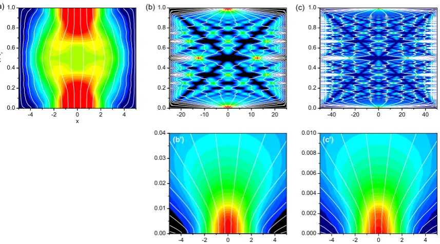
If we now go to the corresponding quantum carpets, displayed in Fig.6forL=w,L=5wand
395
L =10w, we notice an increasing degree of complexity and structuring with increasingL, which is
396
expected as the number of eigenfunctions involved, and hence the number of frequenciesωα,α0, also
397
increases. This gives rise to a highly noisy dynamics, as seen through the corresponding Bohmian
398
trajectories, which comes from the fact that interference traits become more prominent due to the
399
appearance of more profiled dips and ridges [compare panels (b) and (c)], which forces the trajectories
400
to jump relatively fast from some regions to others, since the velocity field is too large in between.
401
Nonetheless, for short times, of the order of 1/25 of theτrcorresponding to the case ofL=5wand
402
1/100 of the one corresponding toL =10w, we find a very similar early-time evolution, as seen in
403
panels (b’) and (c’), respectively, which is in correspondence with the fact that at these stages there is
404
not time enough yet to notice the fine structuring effect coming from all the main contributions (many
405
more in the latter case than in the former, as seen in the upper panels).
406
4. Concluding remarks 407
From a dynamical viewpoint, we have that the delocalization of a released matter wave is
408
analogous to the diffraction it undergoes after crossing an opening — in this latter regard, the opening
1 10 100 1000 0.00
0.01 0.02 0.03 0.04 0.05 0.06 0.07
1 10 100 1000
1E-15 1E-12 1E-9 1E-6 1E-3 1
|cα
|
2
n
(a)
1 10 100 1000
0.0 0.2 0.4 0.6 0.8 1.0
(b) PN
N
(c)
〈
H
〉N
N
Figure 5. (a) Weights|cα|2associated with each one of the components (n, withα =2n−1) used in the reconstruction of a half-cosine squared inside a box with different lengths: L = 10 (black squares)L = 50 (red circles),L = 100 (blue triangles), andL = 200 (red diamonds). For a better visualization, log-log scale has been used in both axes. (b) ProbabilityPNas a function of the numberN of eigenfunctions for the cases cases considered in panel (a). (c) Expectation value of the Hamiltonian,
hHiN, as a function of the numberNof eigenfunctions. In all cases, the shutter width isw=10 and the system massm=1 (with ¯h=1).
would act as the localizing element and its subsequent crossing would play the role of the release. On
410
the other hand, regardless of the initial physical context considered (whether a trapped atomic cloud
411
or a diffracted atomic or molecular beam), if some extra boundaries are added, the new confining
412
conditions will produce the appearance with time of a series or recurrences. The pattern that develops
413
with time is commonly known as a quantum carpet, which displays some symmetries in both space
414
and time according to the interference of the wave with the new confining boundaries. Actually,
415
at some time, a full revival of the initial state (except for a global phase factor) is observed, which
416
is repeated in time once and again unless some dissipative or decohering mechanisms act on the
417
system. This is particularly remarkable in the case of the well-known problem of the particle in a
418
one-dimensional box, assuming such a particle is nonrelativistic, spinless and with massm.
419
In this work we have focused on this classical problem with the purpose to determine which are
420
the main elements that affect the evolution of the bound diffraction process, and more specifically how
421
such elements influence the symmetry displayed by the wave function and its associated flux along
422
their evolution. To that end, we have combined the standard spectral decomposition of the initially
423
localized state in terms of coherent superposition of energy eigenstates with a Bohmian description
424
of its eventual dynamics. Indeed, the possibility to decompose the initial state in this way has been
425
profitably used to devise a simple and efficient analytical algorithm that makes easier and more
426
accurate the computation of velocity fields (flows) and trajectories, since the value of the associated
427
velocity field can be exactly obtained at each position of the configuration space.
428
As it has been shown, these two tools (spectral decomposition and Bohmian trajectories) constitute
429
two rather suitable tools to explore and analyze the problem of the formation of space-time patters
430
inside the cavity in terms of the three key elements that rule the bound diffraction process and the
431
consequent matter-wave dynamics: the shape of the initial wave function, the mass of the particle
432
considered, and the relative extension of the initial state with respect to the total length spanned by
433
the cavity. Specifically, from the spectral decomposition we have been able to identify how each one
434
of these elements contributes to the superposition that generates the corresponding localized matter
435
wave as well as to its eventual evolution; the Bohmian analysis, on the other hand, reveals aspects
436
connected to the diffraction dynamics and the subsequently developed interference traits, such as the
437
origin of the characteristic symmetries displayed by these systems or the appearance of recurrences
438
and full revivals of the initial state. Furthermore, we have also observed that, because of the presence
439
of confining boundaries, even in the cases of an increasingly large box length, no Fraunhofer-like
440
diffraction features can ever be observed at any time, as it is the case of the analogous unconstrained
-4 -2 0 2 4 0.0
0.2 0.4 0.6 0.8 1.0
x
t /
r
(a)
-20 -10 0 10 20 0.0
0.2 0.4 0.6 0.8 1.0
(b)
-4 -2 0 2 4 0.00
0.01 0.02 0.03 0.04
(b')
-40 -20 0 20 40 0.0
0.2 0.4 0.6 0.8 1.0
(c)
-4 -2 0 2 4 0.000
0.002 0.004 0.006 0.008 0.010
(c')
Figure 6. Contour-plots showing the quantum carpets displayed by a cosine-squared wave function (see Table1) along its evolution and for different values of the box size: (a)L=w, (b)L=5wand (c)
L=10w. Panels (b’) and (c’) are enlargements of the regions of (b) and (c), respectively, for the same time displayed in panel (a). A set of Bohmian trajectories with equidistant initial positions has also been superimposed in order to illustrate the dynamical evolution of the flux, particularly at the borders of the lattice. In all simulations here: N =200,w=10 andm=1 (with ¯h=1). In the first panel, for a better visualization, the contours have been taken from zero to half the maximum value of the probability density; in all cases, the transition from darker (dark blue) to lighter (red) colors indicates increasing density values.
waves. This is because of the relatively fast development of a phase field spreading through the whole
442
of the box, which becomes faster as the box length becomes larger and larger.
443
The analysis here has been applied to matter waves. However, we would like to highlight that both
444
the methodology and conclusions are also valid in the case of light propagation through optical fibers,
445
where the input (light) state can be constructed by just selecting the appropriate electromagnetic modes.
446
Actually, notice that under paraxial conditions, Helmholtz’s equation, which describes the distribution
447
of electromagnetic energy inside the fiber, acquires the form of a Schrödinger-like equation [20]. This
448
thus opens an alternative procedure to develop efficient Bohmian-based numerical methodologies to
449
explore and control the dynamics of bound quantum and optical systems in a rather simple fashion.
450
Furthermore, a rather direct extension of this work seems to be re-examining the so-called diffraction
451
in time phenomenon [8,9,13,15–17] under (time) confinement conditions [15].
452
Acknowledgments: Financial support from the Spanish MINECO (grant No. FIS2016-76110-P) is acknowledged.
453
Conflicts of Interest:The author declares no conflict of interest.
454
References 455
1. Phillips, W.D. Laser cooling and trapping of neutral atoms. Rev. Mod. Phys.1998,70, 721–741.
456
2. Grimm, R.; Weidemüller, M.; Ovchinnikov, Y.B. Optical dipole traps for neutral atoms.Adv. At. Mol. Opt. 457
Phys.2000,42, 95–170.
458
3. Zeilinger, A.; Gähler, R.; Shull, C.G.; Treimer, W.; Mampe, W. Single- and double-slit diffraction of neutrons.
459
Rev. Mod. Phys.1988,60, 1067–1073.