Node Weight Swallow Swarm Optimization
Convex Node Segmentation (Nws
2
cns) Algorithm
For Distributed 3-D Localization In Wireless
Sensor Networks (Wsns)
A.Nithya, Dr.A.Kavitha
Abstract: Localization is a significant part in the area of Wireless Sensor Networks (WSNs) with the purpose of has introduced important study significance between academia and research community. The task of establishing substantial manages of sensor nodes in WSNs is identified as localization or positioning and is a key issue in today‘s communication systems toward approximation the position of starting point of events. On the other hand, localization is issue in huge scale 3-D WSNs appropriate toward the uneven topology, for example holes in the path, of the network. Recently, spatial convex node detection method is introduced by means of Convex Coverage Support Vector Machine (CCSVM) toward handle this issue. However in CCSVM classifier, Optimization the Number of Convex Pieces becomes extremely hard task. It turns into very hard designed for although minimizing or maximizing a quantity of known criteria or property in the computational geometry. Node Weight Swallow Swarm Optimization Convex Node Segmentation (NWS2CNS) is introduced in this work for handling optimization of number of convex pieces. NWS2CNS is proposed to minimize the number of convex pieces during network segmentation in huge scale 3-D WSNs. NWS2CNS is proposed for increasing higher location accuracy which is obtained by means of using a node inertia weight toward correctly computes the acceleration coefficients. High speed of convergence, solving local extremum, and increased localization accuracy are the advantages of proposed NWS2CNS algorithm. In NWS2CNS algorithm, segmental planes are able to be categorized by means of two steps: inside boundary region and outside boundary region. Once these two steps are optimized subsequently we expand the network segmentation correctly by means of decreased localization error. The proposed localization algorithm moreover is appropriate a new 3-D coordinate transformation algorithm, which helps decreases the errors proposed by means of coordinate integration among subnetworks and increase the localization correctness.
Index TERMS: Convex partition, localization, Wireless Sensor Networks (WSNs), Swallow Swarm Optimization (SSO), and Node Weight Swallow Swarm Optimization Convex Node Segmentation (NWS2CNS).
————————————————————
1.
INTRODUCTION
Wireless Sensor Networks (WSNs) are collected of a huge number of sensor nodes by means of sensing, computing, and wireless communication abilities. They are extensively used in some of the applications like military applications, environmental monitoring, smart home, and extra areas [1]. Interestingly, the position service of WSN is a promise of significant services such as data gathering, target tracking, and data management. Simply by attaining the position of the sensor node related toward the collected data determination the information construct sense. Consequently, attaining the position data of sensor nodes turn into mainly significant in WSNs [2]. Until now, the several recent localization methods of WSNs are categorized into two types: based [3-4] and range-free [5-6]. Range-based methods make use of distance or angle estimates in their position‘s estimations, at the same time as range-free methods simply make use of connectivity data among unknown nodes and landmarks. Some of the Range-based methods are Received Signal Strength (RSS), Time of Arrival (TOA), Time Difference of Arrival (TDoA), or Angle of Arrival (AoA).
For example, the centralized localization methods [7] might be unsuccessful when the network topology of a huge scale WSN is uneven. The uneven network shapes also difficult the results of localization method. This is since the shortest path among nodes might be bent, which would result in considerable errors in path distance estimation and consequently incorrect localization [8].Regard as the issues fetched by means of the abnormality of network topology, a several methods have been introduced in recent works [9]– [10]. Tan et al [11] introduced a convex partitioning protocol in order solve the 2D/3D topology complexity challenge. Three dimensional Multidimensional Scaling Algorithm (3D-MDS) [12] is proposed and it is proficient of approximating node position in a 3D scenario. To review, the recent schemes are able to hardly work successfully and capably in a distributed way by means of connectivity data simply in a huge-scale 3D WSN of irregular topology. This work handles the above-mentioned issues by introducing a distributed 3D localization algorithm in a huge-scale 3D WSN. Particularly, as a 3D sensor network produces better, it turns into more difficult in topology on description of its close relations by means of the neighboring deployment framework. Node Weight Swallow Swarm Optimization Convex Node Segmentation (NWS2CNS) is introduced in this work for handling the optimization of number of convex pieces in large scale 3-D WSNs. NWS2CNS is introduced for increasing location accuracy which is attained by means of using a node inertia weight toward precisely compute the acceleration coefficients. Sub-optimal network partition is also performed by means of precisely recognizing the concave nodes which decomposes a 3D WSN into a number of estimated convex subnetworks.
_________________________________________
A.Nithya[1].,M.Sc.,M.Phil.,(Ph.D).,
Assistant Professor,
PSGR Krishnammal College for Women,
Coimbatore-641004.
Dr.A.Kavitha[2],
Associate Professor, Department of Computer Science,
2.
LITERATURE REVIEW
Chen et al [13] introduced a new localization schema and increase the Distance Vector (DV)-Hop algorithm by means of introducing a differential error correction scheme with the purpose is introduced to decrease the error of localization collected over numerous hops. The proposed method is able to increase accuracy of location by reducing communication traffic and time complexity. Liu et al [14] introduced a new estimation algorithm and increase the DV-Hop algorithm by means of considering the associations among the communication ranges and the hop-distances. Simulation results demonstrate that the performance of the proposed DV-Hop algorithm is superior when compared to othr methods. Liu et al [15] introduced a modified DV-Hop localization to decrease the error of localization. It makes use of a novel average hop size estimate algorithm, in which the local property of hop-size designed for a particular pair of beacon nodes is used. Results show with the purpose of the modified DV-Hop algorithm works better than the conventional DV-Hop algorithm, particularly when the contribution of local hop-size is selected practically. Pedersen et al [16] developed to introduce a Variational Message Passing (VMP) algorithm with a mean field solution toward the assessment of the posterior probabilities of the sensor positions in an R2 development. Addition toward R3 is straight-forward. VMP algorithm features significantly lesser communication overhead among sensors and predictable mean localization error of the algorithm stabilizes after around 30 iterations when compared to non-parametric methods depending on belief propagation. Noureddine et al [17] introduced a new result by means of two major steps: Initially, a new variant of the Nonparametric Belief Propagation algorithm is introduced for approximating the beliefs. This deviation is performed depending on Monte-Carlo integration by means of rejection sampling where a delimited space region is computed for each node towards to decrease the rejection ratio. This result has the merit of decreasing the quantity of communicating particles and the computation cost. Fan et al [18] introduced a distributed 3D localization scheme designed for an irregular WSN via multidimensional scaling (D3D-MDS). The D3D-MDS algorithm makes use of clusters toward remove the multihop distance errors produced by means of coordinate integration among clusters and increases the accuracy of localization. It also shows that the results with reduced computational complexity compared when compared to other centralized localization methods. Raguraman et al [19] developed a Dimensionality based Particle Swarm Optimization (DPSO) and Hybrid DPSO (HDPSO) includes every dimension of the contributing co-ordinate for particle use to achieve the optimized values in single dimension. This method performs well on random test cases in heterogeneous environments with improved network lifetime. Liu et al [20] introduced a new Approximate Convex Decomposition Localization (ACDL) protocol, by means of dependence on network connectivity information simply. Convex decomposition needs simply local information and shows with the purpose of it has low message overhead. Every convex part of the network, an enhanced MDS algorithm is introduced to calculate a relative location map. Lastly results demonstrate that the efficiency of ACDL by means of wide simulations. Fan et al [21] developed a new method which includes of
two major steps, segmentation and joint localization. In specific, the entire WSN network is divided into numerous subnetworks by means of introducing the approximate convex partitioning. A spatial convex node recognition method is introduced toward support the network segmentation, which depends on the connectivity information simply. Subsequently, every subnetwork is precisely localized by means of using the multidimensional scaling-based algorithm. Extensive simulation results show that this algorithm is able to successfully segment a complex 3-D WSN and considerably increase the localization rate when compared with other existing solutions.
3.
PROPOSED METHODOLOGY
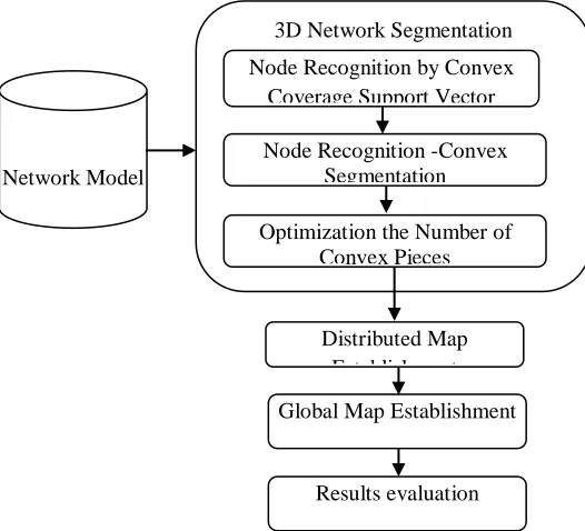
Node Weight Swallow Swarm Optimization Convex Node Segmentation (NWS2CNS) is introduced in this work for handling the optimization of no.of nodes for convex pieces for the duration of network segmentation in huge scale 3-D WSNs. High speed of convergence, escaping as of falling addicted to local extremum, and improved localization accuracy are the advantages of proposed NWS2CNS algorithm. In NWS2CNS algorithm, segmental planes are able to be categorized by means of two steps: inside boundary region and outside boundary region. Once these two steps are optimized subsequently, we expand the network segmentation precisely by means of decreased localization error. NWS2CNS is proposed for increasing the superior location accuracy which is attained by means of using a node inertia weight toward exactly computes the acceleration coefficients. The MDS algorithm is proposed toward attain qualified localization in every subnetwork. Lastly, the proposed algorithm unifies position of each and every one the subnetworks. The overall representation of the proposed work is illustrated in figure 1.
FIGURE 1. ARCHITECTURE OF THE PROPOSED
SYSTEM
Network Model
3D Network Segmentation
Node Recognition by Convex Coverage Support Vector
Distributed Map Establishment
Global Map Establishment Node Recognition -Convex
Segmentation
Optimization the Number of Convex Pieces
The proposed schema includes of the subsequent three steps:
1) Step 1: 3D Network Segmentation: Complete network decomposes a 3D WSN addicted to several predictable convex pieces. It includes of spatial concave node detection by means of classifier, segmentation and partition detection. The amount of partitions optimization is conversed in this partition moreover.
2) Step 2: Distributed Map Establishment: An advanced Multidimensional Scaling Algorithm (MDS) algorithm is used toward confine relative localization designed for every estimated convex part.
3) Step 3: Global Map Establishment: Lastly, combine each
and every one the partitions addicted to a global map and recognize the absolute coordinates of convex pieces. A process which is motivated by means of camera calibration standard of processor vision is introduced. This coordinate merging method is able to decrease the errors of coordinate integration among sub networks and increase the localization accuracy.
Step 1: Network Segmentation
Network segmentation is introduced in order to split an amount of approximate convex pieces. It includes three major steps which are concave node identification, segmentation and partition identification as follows.
1) Concave Nodes identification: A CONCAVE node is a node where the internal angle (the angle spanning transversely the sensing area) is higher than π [20].
Feature I: The spatial coverage of a concave node by means of k hops includes the hugest number of nodes, when compared with the normal boundary nodes. In a 3D WSN where nodes are evenly organized, a boundary node with the purpose of has a better coverage and indicates with the purpose of the node have more neighbors in k steps. Usually, sensor nodes are not evenly distributed in a WSN. As such, describe relative coverage rate is introduced toward hold the result of network density.
∑
(1)
{ ∑
(2)
where Biis denoted as the background distribution density of node i . is represented as the amount of neighboring node used for node i in j steps, and n is represented as the boundary neighbor amount of node i in one step.
Feature II: The highest arc length of a spatial concave node is higher than the usual boundary nodes, and the maximum arc is able to be regarding described as the route starting the left kth neighbor toward the right kth neighbor. Describing the idea of path concavity and compute the path concavity used for every candidate chosen subsequent to rough selection.
(3)
Where k is defined as a radius of k steps, dhopis represented as the average length of one step, and Arci is defined as the
longest arc length which integrates node neighbors in k steps. When (i.e., the central angle is higher than ), set node ias a concave node; else, remove node i. Convex Coverage Support Vector Machine (CCSVM) is introduced for node identification. CCSVM is extension of the previous work [22].
Step 2: Convex Segmentation
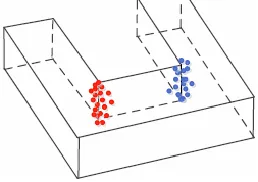
Convex segmentation used in order to decompose a WSN ‗W‘consisting of concave nodes into anumber of convex pieces. As shown in Figure 2, the original concave set is able to be divided into two concave subsets which are describedby means of red and blue nodes, correspondingly.
FIGURE 2. PRINCIPLE OF SEGMENTATION
Logically, the hop distance among red concave nodes are lesser than the step length from a red concave node toward a blue one. It recognizes with the purpose of the inter-class distance is varied from the intra-class distance. From this work we only need to set an opposite distance threshold toward classify each and every one the concave nodes.
Step 3: Optimization the Number of Convex Pieces
relates to the next circumstances. For the initial case, there is no doubt with the purpose of the segmentation step be able to terminate and two convex subnetworks be able to computed because of plane ω. On the other hand, for the next case, the number of convex subnetworks determination is four. In a restricted area, two intersected segmental planes point toward with the intention of the concave regions are very close toward each other and the direction of each plane must not be parallel. It indicates with the purpose of this area may be overly segmented. NWS2CNS algorithm is performed based on the group progress of swallows and the interaction among flock members depending on the concave nodes. NWS2CNS algorithm together with the make use of three categories of particles: Explorer Particles (epi), Aimless Particles (api), and Leader Particles (lpi), each of which has definite characters in the group depending the concave nodes optimization. The epi particles are dependable for searching the issue space depending on the concave node‘s optimization. They perform this exploring behavior for concave nodes optimization with the control of a number of parameters [23]:
1. Location of the local leader depending on the concave node‘s optimization.
2. Location of the global leader depending on the concave node‘s optimization.
3. The greatest individual experience next to the path depending on the concave node‘s optimization.
4. The earlier path depending on the concave node‘s optimization.
The particles make use of the subsequent equations for finding optimal chosen of concave nodes and ongoing the path:
( )
( )(4)
Eq. (4) describes the velocity vector variable in the path of the global leader.
* ( ) +(5)
Eqs. (5) and (6) computes the acceleration coefficient variable ( ) which straightforwardly affects individual results of every particle for best choice of concave nodes
{
( )( ) (
( )
)
( )( ) (
( )
( ) )
( ) (
( ) )
(
6)
* ( ) +(7)
{
( )( ) (
( )
)
( )( ) ( ( )
( ) )
( ) (
( ()) )
(8)
Eqs. (7) and (8) calculate the acceleration coefficient variable ( ) which directly impacts the collective experiences of each particle for optimal selection of concave nodes. These coefficients are quantified regard as
the location of each particle in relation in the direction of the greatest individual experience by means of optimal chosen of concave nodes and the global leader [23]. The opi particles contain a totally random behavior in the setting for best chosen of concave nodes. As a straightforward, this particle enhances the possibility of discovery for optimal chosen of concave nodes the particles which have not been discovered by means of the epi particles. In addition, if other particles obtain fixed in a best local position, there is optimism with the purpose of these particles save them. These particles make use of the subsequent Eq. (9) designed for random movements [23]:
* (* + ( )
() +(9)
In the proposed algorithm there are two categories of leaders: the local leader and the global leader. The particles are categorized addicted to groups. The particles in every group are frequently related for best chosen of concave nodes. Subsequently, the best particle in every group is selected and is named the local leader for greatest concave nodes chosen. Subsequently, the best particle between the local leaders is preferred and is named the global leader used for optimal concave nodes chosen. The particles modify their way and converge related in the direction of the location of these particles.
Node weight
The association of particles in the NWS2CNSbased on some constraints: the position associated toward the problem, the best individual knowledge for optimal concave nodes chosen in every particle, the location of every particle in local groups, and the learn of the best location of every particle among each and every one of the groups for best concave nodes chosen. These constraints find out the communication of every particle with further particles for optimal concave nodes selection. Subsequent to discovering appropriate best concave nodes chosen, particles tend toward meet around it. Here, one of the major significant constraints with the purpose of computes the speed of convergence is the inertia weight and it is used for optimal concave nodes chosen. From the recent work [24– 25], the node weight participates the most important part in computing the localization accuracy for optimal concave nodes chosen. In the proposed algorithm, a node weight is used with the purpose of possesses together of the optimal concave nodes chosen. Eq. (10) shows this inertia coefficient [26].
,( ) *
( )
+ -
[
( )] (10)
The present node position of the particle and expresses the node position of the particle between its group for optimal concave nodes chosen.
Step 4: Partition identification
WSN. To attain this goal, follow three major functions such as isolated nodes classification, flooding and extending.
a) Isolated nodes classification: The result of
segmentation phase is able to be giving a usual border plane among two partitions. On the other hand, it is simply an irregular boundary and shouldn‘t point to which partition these nodes truly go to every of them.
Build a thick volume area in order to check the flooding scheme penetrating as of different polyhedron. The isolated nodes are used in order to mark the execution of flooding schema. Let us assume with the purpose of there exist coordinators in every sub-network in order to take charge of partition edge collection, and lastly inform the nodes of the definite partition(s) they belong to them. The coordinators might be random node. In experimentation, each and every one the k-hop neighbors of the segmental nodes, consisting of the segmental nodes themselves, represents a thick volume area. Each and every one those k-hop neighbors are named as volume nodes. Subsequently, no substance segmental node, their neighbor connection is seen as temporary unacceptable from the neighbor matrix. These nodes subsequently are identified as isolated nodes. Subsequently it is effectively classified a sensor node into four types: boundary nodes, isolated volume nodes, isolated segmental nodes and general nodes.
b) Flooding: Selecting a definite number of common nodes
which belong to diverse polyhedron and keeping flooding used for each piece. Recall with the purpose of the number of concave areas is recognized which has been decided in the very first step of convex segmentation and the optimized phase. At lastly, each and every one common node is categorized as common nodes which identify their clustering number.
c) Extending: Segmental volume nodes are still isolated nodes and they should to be categorized toward diverse parts additionally. For this node, create those categorized common nodes expanding their boundaries. For a definite polyhedron P, if a common node, p, is about to P‘s boundary, it recovers its connection by means of volume nodes and expands one-hop toward create those one-hop neighbors in the same group by p. Subsequently, move toward one more polyhedron toward do the similar expansion. The procedure of expansion terminates until each and every one volume nodes are categorized addicted to diverse polyhedrons.
Distributed Map Establishment
Following to the network segmentation step, the 3D WSN is divided to many subnetworks. Every subnetwork is named as WSN group. Let us assume that every subnetwork, there exists a localization coordinator (must be arbitrary node), and the coordinator is in charge of the procedure of local relative map establish obtaining is as the number of sensor nodes in each subnetwork. In each subnetwork, the shortest hop count among two arbitrary adjacent nodes in the whole WSNis able to be founded via the use of the Floyd algorithm, and each and every one of these hop count distances is saved in a distance matrix called by neibMatrix.
Global Map Establishment
Subsequently obtaining the relative map of every group, requirement towards translate the distributed map hooked on a global map. The global map is recognized from integration these diverse groups. The merging method is toward discovery two together groups which have the maximum public nodes and formerly merge them hooked on one cluster [18]. When completely groups are merged into one group, the merging procedure stops and the global map establishment is finished. Finally, completely the complete coordinates of the unidentified nodes have been assessed. In algorithm, select 3D Coordinate Transformation Algorithm as the practice of merging double together clusters.
4.
SIMULATION RESULTS
The simulation results of the proposed DisLoc-NWS2CNS algorithm is shown in this section and implemented in a MATLAB 2014a. The setting of the simulation is established as follows. Firstly, entirely the sensor nodes are randomly positioned in the three-dimensional area of 100 m*100 m*100 m. Furthermore, the communication radius R is established 40 meters through 100 no. of iterations. Individually time sensor nodes are randomly positioned. Completely the sensor nodes have the identical communication range through default, represented via the use of R. Each pair of nodes is associated if the Euclidean distance among them is no higher than R. The results of proposed DisLoc-NWS2CNS algorithm are measured by the localization error ratio which is described as follows. Let d represent the distance among two neighboring nodes added constructed on the recognized coordinates, and let represent the ground-truth distance among the two neighboring nodes.
Performance Metrics
The localization accuracy, positioning coverage, and stability of the algorithms are measured by Localization Error Ratio (LER), Localized Node Proportion (LNP), and Bad Node Proportion (BNP). Bad anchor nodes denote towards unidentified nodes through a localization error greater than their communication radius R.
The location error ratio is well-defined as follows,
| |
(11)
The performance of proposed algorithm is evaluated by means of the average Localized Node Proportion (LNP), which is well-defined as follows.
(12)
BNP = bad/ localized (13)
Figure 3. Anchor nodes vs. LER (Localization Methods)
LER results of 3D localization algorithms such as DisLoc, DisLoc-CCSVM and proposed DisLoc- NWS2CNS is shown in the figure 3. DisLoc- NWS2CNS algorithm performs better than the DisLoc algorithm and DisLoc-CCSVM in terms of Localization Error. Proposed DisLoc- NWS2CNS algorithm gives lower LER of 0.3992, whereas other methods such as DisLoc-CCSVM and DisLoc produces upto0.4509 and 0.5900 for network connectivity of 4 values respectively (Table 1).
Table 1. LER vs. Localization methods(Anchor Nodes)
Anchor Nodes Disloc DisLoc-CCSVM
DisLoc- NWS2CNS
10 0.5900 0.4509 0.3992
20 0.5590 0.4419 0.3875
30 0.5531 0.4359 0.3824
40 0.5390 0.4310 0.3745
50 0.4877 0.4293 0.3720
60 0.4763 0.3980 0.3482
70 0.4634 0.3891 0.3215
80 0.4374 0.3552 0.3019
90 0.4069 0.3325 0.2948
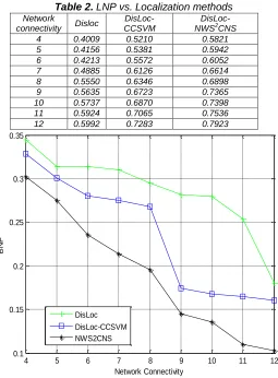
Figure 4. Network connectivity vs. LNP(Localization Methods)
Figure 4 shows the LNP of DisLoc, DisLoc-CCSVM and proposed DisLoc- NWS2CNS algorithm. The DisLoc- NWS2CNS algorithm performs better than the other two algorithms. In DisLoc- NWS2CNS scheme, when the network connectivity comes up to 12, the positioning coverage reaches 0.7923;whereas other method such as DisLoc and DisLoc-CCSVM reaches upto 0.5992 and 0.7283 values respectively (Table 2).
Table 2. LNP vs. Localization methods
Network
connectivity Disloc
DisLoc-CCSVM
DisLoc- NWS2CNS
4 0.4009 0.5210 0.5821 5 0.4156 0.5381 0.5942 6 0.4213 0.5572 0.6052 7 0.4885 0.6126 0.6614 8 0.5550 0.6346 0.6898 9 0.5635 0.6723 0.7365 10 0.5737 0.6870 0.7398 11 0.5924 0.7065 0.7536 12 0.5992 0.7283 0.7923
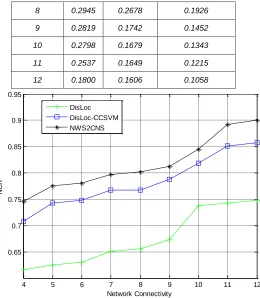
Figure 5. Network connectivity vs. BNP (Localization Methods)
Figure 5 shows the BNP results of localization algorithms are DisLoc, CCSVM and proposed DisLoc-NWS2CNS algorithm. In DisLoc-NWS2CNS scheme, when the network connectivity comes up to 12, the BNP reaches 0.1058, the other methods such as DisLoc-CCSVM, and DisLoc provides 0.1606 and 0.1800 values respectively (Table 3).
Table 3. BNP vs. Localization methods
Network
connectivity Disloc
DisLoc-CCSVM
DisLoc- NWS2CNS
4 0.3446 0.3282 0.3125
5 0.3136 0.3005 0.2852
6 0.3135 0.2804 0.2694
7 0.3101 0.2751 0.2352
10 20 30 40 50 60 70 80 90
0.25 0.3 0.35 0.4 0.45 0.5 0.55 0.6 0.65
Anchor Node Number
L
o
c
a
li
z
a
ti
o
n
e
rr
o
r
DisLoc DisLoc-CCSVM DisLoc-NWS2CNS
4 5 6 7 8 9 10 11 12
0.4 0.45 0.5 0.55 0.6 0.65 0.7 0.75 0.8
Network Connectivity
L
N
P
DisLoc DisLoc-CCSVM DisLoc-NWS2CNS
4 5 6 7 8 9 10 11 12
0.1 0.15 0.2 0.25 0.3 0.35
Network Connectivity
B
N
P
DisLoc
8 0.2945 0.2678 0.1926
9 0.2819 0.1742 0.1452
10 0.2798 0.1679 0.1343
11 0.2537 0.1649 0.1215
12 0.1800 0.1606 0.1058
Figure 6. Network Connectivity vs. Network Coverage Ratio(Localization Methods)
Network Coverage Ratio (NCR) results of the localization algorithms such as DisLoc, DisLoc-CCSVM and proposed DisLoc-NWS2CNS scheme is shown in the figure 6. The DisLoc-NWS2CNS scheme gives higher than the other algorithms. In proposed DisLoc-NWS2CNS scheme, when the network connectivity comes up to 12, the positioning coverage reaches 0.8972, other methods such as DisLoc-CCSVM, and DisLoc gives 0.8573 and 0.7476 gives network connectivity of 12 respectively (Table 4).
Table 4. Network Coverage Ratio vs. Localization methods
Network connectivity
Disloc CCSVM DisLoc- NWSDisLoc- 2CNS
4 0.6159 0.7084 0.7482
5 0.6251 0.7431 0.7725
6 0.6297 0.7482 0.7852
7 0.6509 0.7668 0.7942
8 0.6559 0.7677 0.8039
9 0.6735 0.7877 0.8125
10 0.7380 0.8181 0.8431
11 0.7427 0.8508 0.8843
12 0.7476 0.8573 0.8972
5.
CONCLUSION AND FUTURE WORK
In this work, DisLoc with Node Weight Swallow Swarm Optimization Convex Node Segmentation (NWS2CNS)
protocol is proposed for 3D Wireless Sensor Networks (WSNs). Through correctly recognizing the concave nodes in the topology, suggestion primary decomposes a 3D WSN addicted to a amount of approximate convex subnetworks. At firstly, a spatial convex node identification schema is developed by Convex Coverage Support Vector Machine (CCSVM) towards support the network segmentation, which depends on the connectivity data only. At that pointNWS2CNS is proposed for optimal convex node chosen. In NWS2CNS algorithm, swallows take high swarm intelligence is used for concave nodes optimization, their searching speed is quick, consequently they are able toward fly long distances in order toward immigrate from one node in the direction of another and also, they fly in excessive colonies. At this point, one of the utmost significant parameters with the purpose of regulate the speed of convergence is based on the inertia weight designed for optimum concave nodes choice. The node weight plays the major important role in computing the results for optimal concave nodes chosen. DisLoc- NWS2CNS works in a manner with purpose is distributed with higher accuracy and lesser computation time. From the simulation results it is demonstrated that the proposed DisLoc-NWS2CNSgives higher localization accuracy when compared to existing methods. In the future work a fuzzy control is introduced for tuning of acceleration coefficients.
6.REFERENCES
[1] di Flora, C., Ficco, M., Russo, S. and Vecchio, V., 2005, Indoor and outdoor location based services for portable wireless devices. In 25th IEEE International Conference on Distributed Computing Systems Workshops ,pp. 244-250.
[2] Han, G., Xu, H., Duong, T.Q., Jiang, J. and Hara, T., 2013. Localization algorithms of wireless sensor networks: a survey. Telecommunication Systems, 52(4), pp.2419-2436.
[3] Chen, H. (2008). Novel centroid localization algorithm for threedimensional wireless sensor networks. In Proc. of the 4th international conference on IEEE wireless communications (pp. 1–4).
[4] Liu, K., Wang, S., & Zhang, F. (2005). Efficient localized localization algorithm for wireless sensor networks. In Proc. 5th international conference on computer and information technology (pp. 21–23). [5] Shu, J., Liu, L., & Chen, Y. (2009). A novel
three-dimensional localization algorithm in wireless sensor networks, wireless communications, networking and mobile computing. In Proc. 5th international conference on wireless communications (pp. 24–29).
[6] Zheng, S., Kai, L., & Zheng, Z. H. (2008). Three dimensional localization algorithm based on nectar source localization model in wireless sensor network. Application Research of Computers, 25(8), 2512–2513.
[7] S. Lederer, Y. Wang, and J. Gao, ―Connectivity-based localization of large-scale sensor networks with complex shape,‖ ACM Trans. Sensor Netw., vol. 5, no. 4, p. 31, 2009.
[8] M. Li and Y. Liu, ―Rendered path: Range-free localization in anisotropic sensor networks with
4 5 6 7 8 9 10 11 12 0.65
0.7 0.75 0.8 0.85 0.9 0.95
Network Connectivity
NCR
holes,‖ IEEE/ACM Trans. Netw., vol. 18, no. 1, pp. 320–332, Feb. 2010.
[9] ZhangS., G. Tan, H. Jiang, B. Li, and C. Wang, ―On the utility of concave nodes in geometric processing of large-scale sensor networks,‖ IEEE Trans. Wireless Commun., vol. 13, no. 1, pp. 132– 143, 2014.
[10] JinM., S. Xia, H. Wu, and X. Gu, ―Scalable and fully distributed localization with mere connectivity,‖ in Proc. IEEE INFOCOM, 2011, pp. 3164–3172. [11] TanG., H. Jiang, S. Zhang, Z. Yin, and A.-M.
Kermarrec, ―Connectivitybasedand anchor-free localization in large-scale 2D/3D sensor networks,‖ACM Trans. Sensor Netw., vol. 10, no. 1, p. 6, Nov. 2013.
[12] Shang Y. and W. Ruml, ―Improved MDS-based localization,‖ in Proc.IEEE INFOCOM, vol. 4. Mar. 2004, pp. 2640–2651.
[13] Chen, H.; Sezaki, K.; Deng, P.; So, H.C. An Improved DV-Hop Localization Algorithm with Reduced Node Location Error for Wireless Sensor Networks. IEICE Trans. Fundam. 2008, 91, 2232– 2236.
[14] Liu, M.; Bao, Y.; Liu, H. An Improvement of DV-Hop Algorithm in Wireless Sensor Networks. J. Microcomput. Inf. 2009, 25, 128–129.
[15] Liu, K.; Yan, X.; Hu, F. A modified DV-Hop localization algorithm for wireless sensor networks. In Proceedings of the IEEE International Conference on Intelligent Computing and Intelligent Systems, Shanghai, China, 2009; Volume 3, pp. 511–514.
[16] Pedersen, C.; Pedersen, T.; Fleury, B.H. A variational message passing algorithm for sensor self-localization in wireless networks. In Proceedings of the IEEE International Symposium on Information Theory Proceedings, St. Petersburg, Russia, 2011; pp. 2158–2162.
[17] Noureddine, H.; Gresset, N.; Castelain, D.; Pyndiah, R. A new variant of Nonparametric Belief Propagation for self-localization. In Proceedings of the 17th International Conference on Telecommunications, Doha, Qatar, 2010; pp. 822– 827.
[18] FanJ., B. Zhang, and G. Dai, ―D3D-MDS: A distributed 3D localization scheme for an irregular wireless sensor network using multidimensional scaling,‖ Int. J. Distrib. Sensor Netw., vol. 2015, no. 7, pp. 1–10, 2015.
[19] Raguraman, P., Ramasundaram, M. and Balakrishnan, V., 2018. Localization in wireless sensor networks: A dimension based pruning approach in 3D environments. Applied Soft Computing, 68, pp.219-232.
[20] Liu, W., Jiang H., W. Liu, and C. Wang, ―An approximate convex decomposition protocol for wireless sensor network localization in arbitrary-shaped fields,‖ IEEE Trans. Parallel Distrib. Syst., vol. 26, no. 12, pp. 3264–3274, Dec. 2015.
[21] Fan, J., Hu, Y., Luan, T.H. and Dong, M., 2017. DisLoc: A convex partitioning based approach for distributed 3-D localization in wireless sensor
networks. IEEE Sensors Journal, 17(24), pp.8412-8423.
[22] Nithya A. and Dr.A. Kavitha, ―Convex Coverage Support Vector Machine (CCSVM) Classifier and Distributed 3-D Localization in Wireless Sensor Networks (WSNs)‖, Journal Advanced Research in Dynamical and Control Systems ,Volume 11 ,Issue 5 , pp. 33-43.
[23] Neshat Mehdi, SepidnamGhodrat, Sargolzaei Mehdi. Swallow swarm optimization algorithm: a new method to optimization. Neural Comput Appl 2013;23(2):429–54.
[24] Feng CS, Cong S, Feng XY. A new adaptive inertia weight strategy in particle swarm optimization. In: IEEE Congress on evolutionary computation, CEC 2007; 2007. p. 4186–90.
[25] Li HR, Gao YL. Particle swarm optimization algorithm with exponent decreasing inertia weight and stochastic mutation. 2009 Second international conference on information and computing science. IEEE; 2009. p. 66–9.