http://www.sciencepublishinggroup.com/j/ijdst doi: 10.11648/j.ijdst.20170301.11
ISSN: 2472-2200 (Print); ISSN: 2472-2235 (Online)
A Hesitant Fuzzy Based Medical Diagnosis Problem
Bahram Farhadinia
Department of Mathematics, Quchan University of Advanced Technology, Quchan, Iran
Email address:
[email protected], [email protected]
To cite this article:
B. Farhadinia. A Hesitant Fuzzy Based Medical Diagnosis Problem. International Journal on Data Science and Technology. Vol. 3, No. 1, 2017, pp. 1-7. doi: 10.11648/j.ijdst.20170301.11
Received: February 5, 2017; Accepted: March 19, 2017; Published: April 18, 2017
Abstract.
In this paper, we refine the definition of weighted hesitant fuzzy set (WHFS), the concept that allows the membership of a given element is defined in terms of several possible values together with their importance weight, and then introduce some correlation measures for WHFSs. To illustrate the application of proposed correlation measures for WHFSs, we give a practical example in medical diagnosis.Keywords:
Weighted Hesitant Fuzzy Set, Correlation Measure, Medical Diagnosis Problem1. Introduction
A new generalization of fuzzy set called hesitant fuzzy set (HFS) (Torra (2010)) has received great attention in handling decision making problems where the decision makers have some hesitations among several possible memberships for an element to a set. However, HFS (Torra (2010)) has its inherent drawbacks, because it expresses the membership degrees of an element to a given set only by possible values without emphasizing on the importance of each possible value. In many practical decision making problems, the information provided by decision makers who are familiar with the area might often be described by the same preferences. In such situations, the value repeated several times is more important than that appeared only one time. Thus, the importance of possible membership degrees (i. e., their repetition rate) should be considered in improving the definition of HFS. To consider this fact, Zhang and Wu (2014) introduced the concept of a weighted hesitant fuzzy set, denoted hereafter by (Z-WHFS).
In this contribution, we will show that Zhang and Wu’s definition of union, intersection, addition and multiplication operations for Z-WHFS have not been correctly set up. This motivates us to modify and emend a fault of WHFS definition proposed by Zhang and Wu (2014) so as not only the modified definition of WHFS is acceptable in accordance with the well-known axioms for mathematical operations, but also it allows that all information measures are to be defined reasonably as well as those defined for HFSs Farhadinia
(2014a)-Farhadinia (2014e), and Farhadinia and Ban (2013). In this paper, we develop some correlation measures for WHFSs and then, the proposed correlation measures are applied to a medical diagnosis problem.
The present paper is organized as follows: Section 2 introduces some concepts related to WHFSs. Section 3 is presented a number of correlation measures of WHFSs. Section 4 shows the application of correlation measures in medical diagnosis problems. This paper is concluded in Section 5.
2. WHFS Conceptions
Definition 2.1. (Torra (2010)) Let X be a reference set, a HFS A on X is defined in terms of a function h (x) when applied to X returns a subset of [0, 1], i. e.
A = 〈x, h (x)〉x ∈ X ,
where h (x) is a set of some different values in [0, 1], representing the possible membership degrees of the element x ∈ X to A.
For convenience, we call h (x) a hesitant fuzzy element (HFE) (Xia and Xu (2011)) and denoted briefly by h .
If, for two HFEs h , h , L(h ) ≠ l(h ), then l =
max L(h ), l(h ) . To have a correct comparison, the two HFEsh andh should have the same length l. If there are fewer elements in h than in h , an extension of h should be considered optimistically/pessimistically by repeating its maximum/minimum element until it has the same length with
h .
Hereafter, we assume that all HFEs have the same length N, and let h = ∪ hσ( ) throughout the paper.
As can be seen from Definition 2.1, HFS expresses the membership degrees of an element to a given set only by several real numbers between 0 and 1 of equal importance, while in many real-world situations assigning exact values without importance weight to the membership degrees does
not describe properly the imprecise or uncertain decision information. Thus, it seems to be difficult for the decision makers to rely on the present form of HFSs for expressing uncertainty of an element. To overcome the difficulty associated with the present form of HFSs, Zhang and Wu (2014) have attempted to introduce the concept of weighted hesitant fuzzy set (Z-WHFS) in which the membership degrees of an element to a given set can be expressed by several possible values together with their importance weight.
Definition 2.2. (Zhang and Wu (2014)) Let X be the universe of discourse. A Zhang and Wu’s representation of weighted hesitant fuzzy set (Z-WHFS) on X is defined as
w = 〈x, w (x)〉: x ∈ X = !〈x,γ ∈ w (x) #γ , w∪ $% & 〉 ∶ x ∈ X(, (1)
where w (x) is a set of some different values in [0, 1], denoting all possible membership degrees of the element x ∈ X to the set w , w$γ ∈ )0,1,is the weight of γ such that∑γ. ∈/0.($)w$γ = 1 for any x ∈ X. Zhang and Wu (2014) called w (x) =∪γ. ∈/0.($) #γ , w$γ & a weighted hesitant fuzzy element (Z-WHFE). A Z-WHFE is conveniently denoted byw =∪γ. ∈/0. #γ , wγ & . Zhang and Wu (2014) defined for three Z-WHFEs w =∪% ∈/0 #γ, w% & , w =∪% ∈/01 #γ , w%1& and w =∪% ∈/02 #γ , w%2& some operations as follows: w 3=γ ∈ w∪ #1 − γ, w%& ; (2)
w ∪ w =γ ∈ w ∪, γ ∈ w #max γ1, γ2 , w%1. w%2& ; (3)
w ∩ w =γ ∈ w ∪, γ ∈ w #min γ1, γ2 , w%1. w%2& . (4)
w :=γ ∈ w∪ #γ;, w%& ; (5)
λw =γ1 ∈ w ∪, γ2 ∈ w #1 − (1 − γ); , w %& ; (6)
w ⊕ w =γ ∈ w ∪, γ ∈ w #γ + γ − γ γ , w%1. w%2& ; (7)
w ⊕ w =γ ∈ w ∪, γ ∈ w #γ γ , w%1. w%2& . (8)
By taking the above mathematical operations into consideration, one can easily find that Zhang and Wu (2014) were careless about their definition of operations because such definitions inherit some fundamental disadvantages (see, Farhadinia (2017)).
Here, consider the Z-WHFE w = 〈0.7,0.6〉, 〈0.8,0.4〉 . Then,
w ⊕ w = 〈0.91,0.36〉, 〈0.94,0.48〉, 〈0.96,0.16〉 ≠ 2w = 〈0.91,0.6〉, 〈0.96,0.4〉 ;
w ⊕ w = 〈0.49,0.36〉, 〈0.56,0.48〉, 〈0.64,0.16〉 ≠ w 2
= 〈0.49,0.6〉, 〈0.64,0.4〉 .
Here, in order to avoid the disadvantages arising from Zhang and Wu’s definition of WHFS and mathematical operations on WHFSs, we redefine a weighted hesitant fuzzy set as follows.
w = 〈x, w (x)〉: x ∈ X = F〈x,1 ≤ j ≤ L∪ $F〈 hI( )(x), wI( ) (x)〉J 〉 ∶ x ∈ XJ, (9)
Where w (x), referred to as the weighted hesitant fuzzy element (WHFE), is a set of some different values in [0, 1],denoting all possible membership degrees of the element x ∈ X to the set w , wI( ) (x) ∈ )0, 1, is the weight of hI( ) (x) such that ∑ KL wI( ) (x) = 1 for any x ∈ X. It is interesting to note that if we take wI( ) (x) = ⋯ = wI(KL) (x) = KL for any x ∈ X, then the WHFS w is reduced to a typical HFS. Hereafter, for the convenience of representation, we denote the WHFE w (x) by w =∪ KLF〈hI( ), wI( ) 〉J. Assumption 2.2. Notice that the number of values in different WHFEs may be different. Suppose thatl(w (x)) stands for the number of values in w (x). Hereafter, the following assumptions are made: (A1) All the first component of elements in each w (x) are arranged in increasing order, and then hσ( ) (x) is referred to as the jth largest value in w (x). (A2) If, for some x ∈ X, l(w (x)) ≠ l(w (x)), then L$= max Fl Nw (x)O , l(w (x))J. To have a correct comparison, the two WHFEs w (x) and w (x) should have the same length L$. If there are fewer elements in w (x) than in w (x), an extension of w (x) should be considered optimistically by repeating the maximum first component of elements associated with zero weight until it has the same length with w (x) This kind of extension is quite reasonable since the added element with zero weight is meant to be an element that does not really exist. Throughout this paper, we assume that all WHFEs have the same length N, and let w =∪ 〈hσ( ), wσ( ) 〉 . Definition 2.4. Let w =∪ 〈hI( ), wI( ) 〉 , w =∪ F〈hI( ), wI( ) 〉Jand w =∪ F〈hI( ), wI( ) 〉J be three WHFEs. Then, some operations on the WHFEsw , w and w are defined as the following: w 3Q ∪ 〈 R S(T),/ S(T)〉 ; (10)
w ∪ w =1 ≤ j ≤ N F〈maxFh∪ I( ), hI( ) J, #wWWWWWWWWWWWWWWWWWWW〉J;I(V)+ wI(V)& (11)
w ∩ w =1 ≤ j ≤ N F〈minFh∪ I( ), hI( ) J, #wWWWWWWWWWWWWWWWWWWW〉J;I(V)+ wI(V)& (12)
w :=1 ≤ j ≤ N F〈h∪ I( ):, wI( )〉J ; (13)
λw =1 ≤ j ≤ N 〈1 − (1 − h∪ I( ));, wI( )〉 ; (14)
w ⊕ w =1 ≤ j ≤ N F〈h∪ I( )+ hI( ) − hI( )hI( ), (wWWWWWWWWWWWWWWWWWWW〉J;I(V)+ wI(V)) (15)
w ⊕ w =1 ≤ j ≤ N F〈h∪ I( ) hI( ) , (wWWWWWWWWWWWWWWWWWWW〉J,I(V)+ wI(V))
In the above formulas, (wWWWWWWWWWWWWWWWWWWWσ(V)+ wσ(V)) for 1 ≤ j ≤ N, referred to as the normalized weights, are determined in two steps: (i) We first calculate the weight of jth component of the binary operation w ⨀w by simply adding the weights wσ( ) and wσ( ) for 1 ≤ j ≤ N; (ii) After the whole components of w ⨀w are to be obtained, their weights are considered again and then normalized.
Example 2.1. Suppose that
w = 〈0.2,0.1〉, 〈0.4,0.3〉, 〈0.5,0.6〉 and w = 〈0.3,0.5〉, 〈0.7,0.5〉 are two given WHFEs. Bearing Assumption 2.1 in mind, w should be first extended as w = 〈0.3,0.5〉, 〈0.7,0.5〉, 〈0.7,0.0〉 . Then, one gets
w ∪ w = Y〈max 0.2,0.3 ,(0.1 + 0.5)2 〉 , 〈0.7,0.4〉, 〈0.7,0.3〉Z ;
w ∩ w = Y〈min 0.2,0.3 ,(0.1 + 0.5)2 〉 , 〈0.4,0.4〉, 〈0.5,0.3〉Z ;
(w ∪ w ) ∪ w = Y〈max max 0.2,0.3 , 0.2 ,((0.1 + 0.5) + 0.1)3 〉 , 〈0.7,1.13 〉 , 〈0.7,1.23 〉Z ;
(w ∩ w ) ∩ w = Y〈min min 0.2,0.3 , 0.2 ,((0.1 + 0.5) + 0.1)3 〉 , 〈0.4,1.13 〉 , 〈0.5,1.23 〉Z ;
w 1:= 〈0.2;, 0.1〉, 〈0.4;, 0.3〉, 〈0.5;, 0.6〉 ;
λw = 〈1 − 0.8;, 0.1〉, 〈1 − 0.6;, 0.3〉, 〈1 − 0.5;, 0.6〉 ;
w ⊕ w = 〈0.44,0.3〉, 〈0.82,0.4〉, 〈0.85,0.3〉 ; w ⨂w = 〈0.06,0.3〉, 〈0.28,0.4〉, 〈0.35,0.3〉 .
Theorem 2.1. Farhadinia (2017) Let
w =∪ 〈hI( ), wI( ) 〉 , w =∪ F〈hI( ), wI( ) 〉J and w =∪ F〈hI( ), wI( ) 〉J be three WHFEs. Then, all operations w 13, w ∪ w ,w ∩ w , w
1
:, λw , w ⊕ w , w ⨂w given in Definition 2.4 are also WHFEs.
Theorem 2.2. Farhadinia (2017) Let
w =∪ 〈hI( ), wI( ) 〉 , w =∪ F〈hI( ), wI( ) 〉J
and w =∪ F〈hI( ), wI( ) 〉J be three WHFEs. Then,
#w 3&;= (λw )\ ; Nw :O
\
= λ#w 3& ; (16)
(w ∪ w )\= w 1 3∩ w 2 3 ; (w ∩ w )\= w 1 3∪ w 2 3 ; (17)
(w ⊗ w )\= w 1 :⊗ w 2: ; λ(w ⊕ w ) = λw 1⊕ λw 2 ; (18)
(w ⊕ w )\= w 1 3⊗ w 23 ; (w ⊗ w ) \= w 13 ⊕ w 2 3 ; (19)
w ⊕ w = w 2⊕ w 1 ; w ⊗ w = w ⊗ w ; (20)
w ∪ w = w ∪ w ; w ∩ w = w ∩ w ; (21)
w ∪ (w ∪ w ) = (w ∪ w ) ∪ w ; w ∩ (w ∩ w ) = (w ∩ w ) ∩ w (22)
w ∪ w = w ; w ∩ w = w ; (23)
w ⊕ w = 2w ; w ⊗ w = w 2 (24)
3. Correlation Measures for WHFSs
Definition 3.1. A real-valued function ^ is called a correlation measure for WHFSs, if for WHFSs w , w_ on X, ^ satisfies the following properties:
(^2) ^(w , w_) = ^(w_, w ) ;
(^3) ^(w , w_) = 1 `a w = w_. By assuming that
w = 〈x, w (x)〉: x ∈ X = F〈x,1 ≤ j ≤ b F〈 h∪ I( )(x), wI( ) (x)〉J 〉 ∶ x ∈ XJ, (25)
w_= 〈x, w _(x)〉: x ∈ X = F〈x,1 ≤ j ≤ b F〈 h∪ _I( )(x), w_I( ) (x)〉J 〉 ∶ x ∈ XJ, (26)
we define the following correlation measure formulas for any two WHFSs w and w_ as
^c d e f1(w , w_) = ∑ N 1
g∑gTj1 /.S(T) ($h) .S(T)($h) /iS(T) ($h) iS(T)($h)O k
hj1
l∑ Nkhj1 g1∑gTj1( /.S(T) ($h) S(T). ($h))2Ol∑ Nhj1k g1∑gTj1( /iS(T) ($h) S(T)i ($h))2O
, (27)
In order to equip the WHFS theory with further correlation measures, we presented two other correlation measures for WHFSs by extending Jaccard (1901)’s and Dice (1945)’s correlation measures defined on the vector space as follows:
ρw H F S2(w , w_) = qr(1N r wI( ) (xs) h I( )(xs) w_I( ) (xs) h_I( )(xs)) t
sQ t
sQ
u /
Y∑ ( ∑ w wtsQ Q I( ) (xs) h I( )(xs)x +
∑ ( ∑ w wtsQ Q _I( ) (xs) h_I( )(xs)x − ∑ N ∑ wsQt Q I( ) (xs) h I( )(xs) w_I( ) (xs) hI( )_ (xs)OZ, (28)
ρw H F S3(w , w_) = ∑ N 1
g∑gTj1 /.S(T) ($h) .S(T)($h) /iS(T) ($h) iS(T)($h)O k
hj1
∑khj1Ng1∑gTj1( /.S(T) ($h) .S(T)($h))2Oy∑khj1Ng1∑gTj1( /iS(T) ($h) S(T)i ($h))2O.
(29)
Theorem 3.1. Farhadinia (2017) The measure functions
ρWHFSi((w , w_) (i = 1,2,3) given respectively by (27)-(29) are correlation measures for WHFSs w and w_.
4. WHF Information Used in Medical
Diagnoses
In this portion, we implement the following medical diagnosis problem to illustrate the efficiency of the correlation measures for WHFSs.
Example 4.1. Consider the set of diagnoses D = {Viral fever, Malaria, Typhoid, Stomach problem, Chest problem}. The aim here is to assign a patient with the given values of the symptoms, S = {Temperature, Headache, Cough, Stomach pain, Chest pain} to one of the aforementioned diagnoses. Three medical experts El, (l = 1, 2, 3) are invited to provide their possible assessment of diagnoses with respect to symptoms. For each diagnosis with respect to each symptom, all of the medical experts provide anonymously their evaluated values. As an example, for the diagnosis ”Viral fever” with respect to the symptom ”Temperature”, the evaluation value provided by
medical experts E1 and E3 is 0.5; and E2’s evaluation value is 0.7. In this regard, and noting that the weights of three medical experts are unknown, the evaluation of ”Viral fever” with respect to ”Temperature” can be represented by a WHFE as
w (V iralfever, Temperature) = w = !〈0.5,23〉 , 〈0.7,13〉(.
Note that the characteristics of the diagnosis ”Viral fever”
with respect to the
symptoms ”Headache”, ”Cough”, ”Stomach pain”, ”Chest pain”, denoted respectively by WHFEs w , (j = 2, 3, 4, 5), form the WHFS w which is indicated in the first row of Table 1. The results evaluated for other diagnoses with respect to symptoms arecontained in a weighted hesitant fuzzy decision matrix, shown in Table 1.
Table 1. Symptoms characteristic for the considered diagnoses.
Temperature Headache Cough Stomach pain Chest pain
Viral fever !〈0.5,2
3〉 , 〈0.7,13〉( !〈0.3,33〉( !〈0.4,13〉 , 〈0.6,3〉(2 !〈0.3,23〉 , 〈0.4,13〉( !〈0.6,23〉 , 〈0.7,13〉(
Malaria !〈0.4,1
3〉 , 〈0.7, 2
3〉( !〈0.5,
2 3〉 , 〈0.8,
1
3〉( !〈0.5,
3
3〉( !〈0.2,
2 3〉 , 〈0.3,
1
3〉( !〈0.7,
1 3〉 , 〈0.8,
2 3〉(
Typhoid !〈0.3,2
3〉 , 〈0.4,13〉( !〈0.5,13〉 , 〈0.6,23〉( !〈0.1,3〉 , 〈0.4,2 13〉( !〈0.6,33〉( !〈0.5,23〉 , 〈0.7,13〉(
Stomach
problem !〈0.5,
2 3〉 , 〈0.7,
1
3〉( !〈0.5,
2 3〉 , 〈0.7,
1
3〉( !〈0.7,
3
3〉( !〈0.4,
2 3〉 , 〈0.5,
1
3〉( !〈0.5,
1 3〉 , 〈0.8,
2 3〉(
Chest problem !〈0.2,2
3〉 , 〈0.3,13〉( !〈0.4,23〉 , 〈0.7,13〉( !〈0.4,3〉 , 〈0.6,1 23〉( !〈0.3,23〉 , 〈0.4,13〉( !〈0.4,33〉(
Table 2. Symptoms characteristic for the considered patients.
Temperature Headache Cough Stomach pain Chest pain
Al !〈0.4,3
3〉( !〈0.5,23〉 , 〈0.7,13〉( !〈0.6,13〉 , 〈0.7,3〉(2 !〈0.2,23〉 , 〈0.4,13〉( !〈0.1,13〉 , 〈0.2,23〉(
Bob !〈0.6,2
3〉 , 〈0.7,13〉( !〈0.5,13〉 , 〈0.8,23〉( !〈0.5,3〉 , 〈0.6,2 13〉( !〈0.3,33〉( !〈0.4,23〉 , 〈0.5,13〉(
Joe !〈0.2,2
3〉 , 〈0.3,13〉( !〈0.5,33〉( !〈0.2,23〉 , 〈0.4,3〉(1 !〈0.6,13〉 , 〈0.7,23〉( !〈0.5,23〉 , 〈0.7,13〉(
Ted !〈0.4,3
3〉( !〈0.4,23〉 , 〈0.7,13〉( !〈0.3,13〉 , 〈0.4,3〉(2 !〈0.7,23〉 , 〈0.8,13〉( !〈0.5,23〉 , 〈0.6,13〉(
As can be seen from Tables 1 and 2, all WHFEs are not in the same size. To circumvent this issue, we implement Assumption 2.6. In this regard, The WHFEs with fewer elements are extended optimistically by repeating the maximum first component of elements associated with zero weight until it has the same length with others. For example, the WHFE
w (V iralfever, Temperature) : = w = F〈0.3,ƒƒ〉J is extended to F〈0.3,ƒƒ〉 , 〈0.3,0〉J.
During the process of deriving a diagnosis for each patient, the degree of dependence between the rows of Tables 1 and 2 should be analyzed. For instance, the first rows of Tables 1 and 2 which are regarded as the following two WHFSs
Al = hTemperature, !〈0.4,33〉 , 〈0.4,0〉( , 〈Headache, !〈0.5,23〉 , 〈0.7,13〉(〉 , 〈Cough, !〈0.6,13〉 , 〈0.7,13〉(〉,
〈Stomachpain, !〈0.2,23〉 , 〈0.4,13〉(〉 , 〈Chestpain, !〈0.1,13〉 , 〈0.2,23〉(〉 ;
V iralfever = ‰〈Temperature, , !〈0.5, 2
3〉 , 〈0.7,13〉(〉 , 〈Headache, !〈0.3,33〉 , 〈0.3,0〉(〉 , 〈Cough, !〈0.3,13〉 , 〈0.6,23〉(〉 , 〈Stomachpain, !〈0.3,23〉 , 〈0.4,13〉(〉 , 〈Chestpain, !〈0.6,23〉 , 〈0.7,13〉(〉 Š,
are taken into account to determine the correlated degree of Al and viral fever.
In order to proceed, we apply the correlation measure
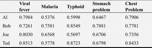
ρWHFS1 to determine the degree of dependence between diagnoses and patients. The results obtained by the use of these correlation measures are shown in Table 3.
Table 3. Values of ^WHFS1 for each patient to the considered set of possible
diagnoses.
Viral
fever Malaria Typhoid
Stomach problem
Chest Problem
Al 0.7984 0.5376 0.5998 0.6467 0.7906
Bob 0.7261 0.7581 0.8549 0.7881 0.7781
Joe 0.8030 0.6568 0.5697 0.6706 0.7356
Ted 0.8513 0.5778 0.8723 0.6798 0.8433
By comparing the results listed in Table 3, we observe that AL and Joe suffer from ”Viral fever”, Bob and Ted from ”Typhoid”.
Table 3 present the same result for all correlation measures.
5. Conclusion
In this contribution, we modified and emended a fault of WHFS definition so as it is acceptable in accordance with the well-known axioms for mathematical operations. We believe many future works can be developed by the use of the findings of this contribution which support the decision makers in making decisions effectively in WHFS-structured MAGDM problems.
Acknowledgements
References
[1] Zhang Zh., Wu Ch. (2014), Weighted hesitant fuzzy sets and their application to multi-criteria decision making, British Journal of Mathematics and Computer Science 4, 1091-1123.
[2] Torra V. (2010), Hesitant fuzzy sets, International Journal of Intelligent Systems 25, 529-539.
[3] Farhadinia B. (2014a), Correlation for dual hesitant fuzzy sets and dual interval-valued hesitant fuzzy sets, International Journal of Intelligent Systems 29, 184-205.
[4] Farhadinia B. (2014b), Distance and similarity measures for higher order hesitant fuzzy sets, Knowledge-Based Systems 55, 43-48.
[5] Farhadinia B. (2013a), A novel method of ranking hesitant fuzzy values for multiple attribute decision-making problems, International Journal of Intelligent Systems 28, 752-767. [6] Farhadinia B. (2013b), Information measures for hesitant
fuzzy sets and interval-valued hesitant fuzzy sets, Information Sciences 240, 129-144.
[7] Farhadinia B. (2014e), An efficient similarity measure for intuitionistic fuzzy sets, Soft Computing 18, 85-94.
[8] Farhadinia B., Ban A. I. (2013d), Developing new similarity measures of generalized intuitionistic fuzzy numbers and generalized interval-valued fuzzy numbers from similarity measures of generalized fuzzy numbers, J. Mathematical and Computer Modelling 57, 812-825.
[9] Farhadinia B. (2017), Utility of correlation measures for weighted hesitant fuzzy sets and weighted interval-valued hesitant fuzzy sets in medical diagnosis problems, submitted to Iranian Journal of Fuzzy Systems.
[10] Xia M., Xu Z. (2011), Hesitant fuzzy information aggregation in decision making, International Journal of Approximate Reasoning 52, 395-407.
[11] Jaccard P. (1901), Distribution de la flore alpine dans le Bassin des Drouces et dans quelques regions voisines, Bulletin de la Socit Vaudoise des Sciences Naturelles 37, 241-272. [12] Dice L. R. (1945), Measures of the amount of ecologic