Video Streaming Analysis in Vienna LTE System Level Simulator

(1)

Video Streaming Analysis in Vienna LTE System Level

Simulator

Zakaria Ye

LIA/CERI University of Avignon 84000, Avignon, France

Tania Jiménez

Rachid El-Azouzi

ABSTRACT

The demand for multimedia services in mobile communica-tion is increasing day by day due to the proliferacommunica-tion of end devices. To overcome the future needs of data communi-cation on mobile devices, the 3rd Generation Partnership Project (3GPP) has introduced a new technology which is known as Long Term Evolution (LTE) UMTS. In this pa-per, we study video streaming behavior on the LTE network. For this purpose, we use the Vienna LTE System Level Sim-ulator which implements network features that correspond to our goal. We consider the parameters that may affect the users experience on a network and define ten scenarios for our simulations. We finally search for methods to fit the video streaming data traffic on the LTE network and exhibit its long range dependence.

Keywords

Video streaming, long term evolution, simulations

1. INTRODUCTION

Over the last few years, cellular networks have attested a rapid growth of multimedia applications, particularly video streaming applications. This growth is due to the prolifera-tion of the end devices and the multimedia content providers like Netflix, Youtube and the video sharing platforms we can find on the social networks. The current networks, i.e., 3G and previous, suffer from this traffic load due to the band-width limitation which is the main constraint of the network operators. To overcome the future needs of data communi-cation on mobiles devices, the 3rd Generation Partnership Project (3GPP) has introduced a technology known as Long Term Evolution (LTE) of Universal Mobile Telecommunica-tions System (UMTS). The LTE performance requirements are a high data rate and spectrum efficiency for both down-link and updown-link transmission, a low latency, a high cell ca-pacity. The major features that distinguish LTE from 3G are the flat-IP archtecture for the core network and the

air-interface. Its main motivation is to guarantee the quality of services (QoS) of the mobile users.

Quality of Experience (QoE) has taken an important in-terest in the performance evaluation of multimedia traffic. Hence the satisfactory QoE to video consumers becomes a key objective for LTE system design. In this paper, we are interested to characterize properties of video streaming traf-fic over LTE. For this purpose, we simulate using the Vienna LTE System Level Simulator. The Vienna LTE simulator implements the different modules of the LTE technology with an abstract physical layer which catches its essential characteristics and decreases the computational level.

The first step towards defining scenarios for the streaming simulations is to understand how the streaming works: We have a video file stored in a media server. When a streaming user requests a video, this video file is divided into chunks transmitted to the user. The user holds a buffer (the play-out buffer), where the video packets are stored to be played. The main component in this procedure is the base station called eNodeB in the LTE technology. The eNodeB hold a buffer for every user within its cell where the upcoming packets from the media server are stored to be transmit. Between the media server and the eNodeB, the streaming packets are transmitted smoothly. That means, in a regular manner. This is not the case for the transmission between the eNodeB and the user because of the air interface. Hence this link becomes the bottleneck for the streaming packets and introduces jitter which degrades the QoS of the stream-ing applications.

2. MOTIVATIONS

Video streaming analysis over wireless networks has been studied for many years. The oldest papers use the video streaming simulation over previous networks architecture us-ing tools such as ns-2, OPNET or OMNET++:

In [1] authors developed a new ns-2 module providing a RTP and RTCP implementation. A model of H.264 video stream-ing is developed usstream-ing the OPNET modeler in [2]. Authors in [3] simulated and compared the delay, packet loss, jitter and throughput of the video streaming over an ADSL and a WiMAX networks.

There are some recent papers that deal with the video stream-ing over the LTE networks. Most of them focus on

(2)

ing. In [4] the performance comparison of three scheduling algorithms is performed while authors in [5] and [6] proposed a scheduling framework for adaptive video and a quality op-timized downlink scheduling respectively. The packet loss modeling is performed for the video streaming over the LTE networks in [7]. In [8] authors performed simulations using ns-3 but they did not model the video traffic, they presented users throughputs as simulation results.

To the best of our knowledge, this paper is the first attempt to address the video streaming traffic modeling since the first release of the Long Term Evolution in 2008. We decide to use the Vienna LTE Simulator that implements only LTE because it was open source and it is easy to customize it.

Our main motivation is to be able to compare theoretic mod-els with the simulation modmod-els. These theoretic modmod-els are used in queueing theory for the computation of some metrics such as the QoS and the quality or experience (QoE).

We also study the Long Range Dependence (LRD) of the video traffic because it exhibits the bursty nature of the video traffic. This traffic is often wrongly modeled as an exponential distribution [9], the LRD shows that the inter-arrivals are not independent.

The rest of this paper is organized as follows: In section 3 we overview the Long Term Evolution. Section 4 presents the Vienna LTE System Level Simulator and section 5 describes the parameters of the simulations, the video traffic modeling and the results. Section 6 concludes this paper.

3. LTE SYSTEM MODEL

The Long Term Evolution (LTE) standard, specified by the 3rd Generation Partnership Project (3GPP) in release 8, is the next step forward in cellular 3G services. LTE offers significant improvements over previous technologies such as Global System for Mobile communications (GSM), Univer-sal Mobile Telecommunications System (UMTS) and High-Speed Packet Access (HSPA) by reforming the core network and introducing a novel physical layer. The main reasons of these changes in the Radio Access Network (RAN) sys-tem design are the need to provide higher spectral efficiency, lower delay and more multi-user flexibility than the currently deployed networks [10].

The architecture of the LTE standard is simpler than those of the previous technologies because it is based on all-IP network. There is the core network and the Radio Access Network which consists of a set of eNodeBs (Bases Stations) and Users Equipements (UEs) which communicate through the air interface. Our work is focused on the RAN layer. There is the interoperability between the LTE network and W-CDMA, GSM systems and non-3GPP systems. Then multimode UEs will support handover to and from these other systems and legacy technologies such as HSPA+ and Enhanced EDGE will continue to operate within the new data infrastructure.

As said before, the LTE introduces a novel physical layer which employs some advanced technologies that are new to cellular applications. These include Orthogonal Frequency Division Multiplexing (OFDM) and Multiple Input Multiple Output (MIMO) data transmission. In addition, the LTE physical layer uses Orthogonal Frequency Division Multiple

Access (OFDMA) on the downlink (DL) and Single Carrier-Frequency Division Multiple Access (SC-FDMA) on the up-link (UL) [11].

We will just consider the downlink channel in this paper be-cause the simulator does not implement the uplink channel but this does not affect our results.

OFDM is a modulation technique. When information is transmitted over a wireless channel, the signal can be dis-torted due to the multipath. Multipath is caused by signal reflection of buildings, vehicules and other obstructions. The multipath effect can cause delays between symbols which results to inter-symbol interference (ISI). OFDM eliminates ISI in the time domain in the following way: OFDM sys-tems break the available bandwidth into many narrower sub-carriers and transmit the data in parallel streams. Each subcarrier is modulated using varying levels of QAM mod-ulation, e.g. QPSK, 16QAM, 64QAM or possibly higher orders depending on signal quality. Each OFDM symbol is therefore a linear combination of the instantaneous sig-nals on each of the subcarriers in the channel. Also OFDM symbols are generally much longer than symbols on single carrier systems of equivalent data rate. Then OFDM symbol is preceded by a cyclic prefix (CP), which is used to effec-tively eliminate ISI. The sub-carriers are very tightly spaced to make efficient use of available bandwidth, yet there is no interference among adjacent sub-carriers (Inter Carrier In-terference or ICI).

(3)

(and hence overall system capacity) and increased data rates for individual users [12]. MIMO has different modes. The spatial diversity exploits the independent fading of different signal paths between the various transmit and receive anten-nas to improve the reliability of a communication link. The spatial multiplexing takes advantage of multipath propaga-tion to create a number of independent transmission chan-nels between the transmitter and receiver, which enables two or more different signal streams to be transmitted si-multaneously. The closed loop feedback and precoding en-ables a transmitter to take advantage of information about the transmission channel, provided by the receiver. The standard exploits the flexibility of MIMO by including the different operating modes and the system is able to switch between them to suit different operating circumstances. With its new system architecture and novel technologies, the LTE system aims to achieve a high throughput and small latency for different services including multimedia applica-tions. We are particularly interested in the video streaming.

4. VIENNA LTE SYSTEM LEVEL

SIMULA-TOR

The Vienna LTE System Level Simulator of the Institute of Telecommunications at the Vienna University of Tech-nology, is an open source software developped in MATLAB using the Object-oriented programming (OOP) capabilities that have been introduced with the release 2008a. The work has been funded by A1 Telekom Austria AG and the Chris-tian Doppler Laboratory for Wireless Technologies for Sus-tainable Mobility. The simulator is available in [13]. The project first develops a link level simulator before upgrad-ing it to a system level simulator. While link-level simula-tions allow for the investigation of issues such as Multiple Input Multiple Output (MIMO) gains, Adaptive Modula-tion and Coding (AMC) feedback, modeling of channel en-coding and deen-coding, system level simulations focus more on network-related issues such as scheduling, mobility han-dling, interference management or signals propagation [14]. Then in system level simulations, the physical layer is ab-stracted from link level results and network performance is studied. To have an overview of the simulator, a schematic block diagram is proposed in Fig.: 1.

The core of the simulator has two parts: a link measurement model and a link performance model. The link measure-ment model abstracts the measured link quality to reduce the computational complexity by pregenerating a lot of pa-rameters (eNodeBs, UEs, schedulers, resource block grids, pathloss and shadow fading maps, UEs fast fading...) be-fore entering the main loop of the simulation. Then these parameters can be re-used during the simulation. The link quality model contains three (3) parts: (i) the macroscopic pathloss between the eNodeBs and the UEs due to the dis-tance and the antenna gain, (ii) the shadow fading due to the obstacles between the eNodeBs and the UEs and (iii) the small-scale fading or fast fading which models the time-dependant process of the channel. The pathloss, shadow fading and fast fading are combined to compute the SINR. On the other hand, the link performance model determines the BLER (Block Error Ratio) at the receiver given a cer-tain resource allocation and Modulation and Coding Scheme (MCS). 15 different MCSs are defined, driven by 15 Channel

base-station deployment antenna gain pattern tilt/azimuth

Link-measurement model

Link-performance model

throughput error rates error distribution link adaptation strategy

precoding micro-scale fading macro-scale fading antenna gain shadow fading interference

structure

mobility management

power allocation strategy resource scheduling

strategy traffic model

network layout

Figure 1: Schematic block diagram of the LTE sys-tem level simulator [14]

Quality Indicator (CQI) values. The CQIs use coding rates between 0.0762 and 0.9258 combined with QPSK, 16-QAM and 64-QAM modulations.

The simulator contains a main matlab file which defines the path of a simulation, it can be summarized in the pseudo-code below [14]:

foreach simulated TTIdo move UEs

if UE outside ROIthen

reallocate UE randomly in ROI foreach eNodeBdo

receive UE feedback after a given feedback delay schedule users

foreach UEdo

1- channel state→link quality model→SINR 2- SINR, MCS→link perf. model→BLER 3- send UE feedback

(4)

5. VIDEO STREAMING ANALYSIS

We perform simulations using the video streaming traffic and different network parameters that affect the dynamics of the mobile communication networks.

Then we use statistical methods to fit the video data traffic using standard density functions.

5.1 Simulation Setup

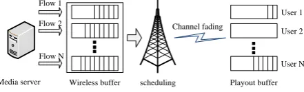
The system model contains three (3) main components. The media server, the base station (eNodeB) and the users. Fig. 2 shows the system architecture with N streaming users. The mobile users request streaming service from servers and the media streams are transmitted by the eNodeB over a fast fading channel. The streaming flow spans a wired link be-tween the media server and the eNodeB. In this link the streams are transmitted in a regular manner. The streams span again a wireless link, between the eNodeB and the mo-bile user, which represents the bottleneck of the transmission because of the channel fading. Each mobile user is associ-ated with only one flow. The system is composed of two types of buffers, the wireless buffer at the eNodeB and the playout buffer at the user side.

Media server Flow 1

Flow 2

Flow N

Wireless buffer scheduling Playout buffer Channel fading

User 2 User 1

User N

Figure 2: Media streaming system in LTE networks

The wireless buffer and the playout buffer work in a tandem way, which means that the departure process of a user in the former is exactly the arrival process in the latter. How-ever, they work at the different time scales and at different layers. The wireless buffer works at the bit level due to the bit loading in the lower layers, and the playout buffer works at the video frame level.

The video streaming server model is integrated in the Vi-enna LTE simulator, in the trafficModel module. Table 1 shows the video traffic model parameters. Each video frame is splited into 8 packets (slices) where packet sizes and inter-arrival between packets follow a truncated Pareto distribu-tion of parameters α and K. K represents the minimal packet size and the minimal inter-arrival between packets. We fix the packet size to 120 bytes and the inter-arrival to 0ms. We assume that the media streams always have back-logged packets in the wireless buffer. This assumption holds due to two reasons: [15] First the online movies are usually very large, ranging from 100MB to 1GB. Second, most of Internet streaming servers use HTTP protocol (over TCP) to deliver streaming packets. TCP congestion control mech-anism exploits the available bandwidth by pumping as more packets as possible to the wireless buffer. Therefore, we can simply regard the wireless buffers to be always saturated.

Information types

Distribution Distribution parameters Inter-arrival time

between the be-ginning of each frame

Deterministic (based on 100fps)

10 ms

Number of packet in a video-frame

Deterministic 8

Video-packet size Truncated Pareto (Max= 120 bytes)

K=120, α

=1.2 Inter-arrival

time between video-packets in a video-frame

Truncated Pareto

(Mean= 0ms,

Max= 0ms)

K=0,α=1.2

Table 1: Video traffic model parameters

For this reason, we fix the inter-arrival between the begin-ning of each frame to 10ms. The media server sends a frame to the eNodeB every 10ms, that is why the inter-arrival be-tween packets are fixed to 0ms because one frame contains 8 packets. This configuration corresponds to a rate of 100fps on the wired link.

We consider a network with a system frequency of 2.14Ghz

and a bandwidth of 20M hz. It is a macro-cells network with 7 eNodeBs. The distance between neighboring eNodeBs is 500m. Each eNodeB covers 3 sectors where a sector is a part of a cell. We use this topology because most of the operators use three sectors sites and by sectoring we gain better control of interference issues. As we said in sec-tion 4, the propagasec-tion model combines the pathloss model, the shadow fading and the channel model. For the channel model, we use theWinner II+based channel from the Win-ner project (one should download and put these files in the simulator before running it). It is a more complete model which covers all the propagation scenarios. The winner+ channel follows a geometry-based stochastic channel mod-eling approach, which allows the creation of an arbitrary double directional radio channel model [16].

(5)

pathloss and environ-ment

shadow fading

channel model

antenna model

number of users (per cell)

walking model

user speed (km/h)

scheduler trans. modes

nRX and nTX

scenario 1

X claussen winner+ kathrein 150 straight 5 alphafair MIMO 2x2

scenario 2

TS36942 urban

X winner+ kathrein 150 straight 5 alphafair MIMO 2x2

scenario 3

TS36942 urban

claussen X kathrein 150 straight 5 alphafair MIMO 2x2

scenario 4

TS36942 urban

claussen winner+ X 150 straight 5 alphafair MIMO 2x2

scenario 5

TS36942 urban

claussen winner+ kathrein X straight 5 alphafair MIMO 2x2

scenario 6

TS36942 urban

claussen winner+ kathrein 150 X 5 alphafair MIMO 2x2

scenario 7

TS36942 urban

claussen winner+ kathrein 150 straight X alphafair MIMO 2x2

scenario 8

TS36942 urban

claussen winner+ kathrein 150 straight 5 X MIMO 2x2

scenario 9

TS36942 urban

claussen winner+ kathrein 150 straight 5 alphafair X 2x2

scenario 10

TS36942 urban

claussen winner+ kathrein 150 straight 5 alphafair MIMO X

Table 2: Simulation parameters

constant speed. When the users are out of the ROI, they are reallocated randomly in the ROI. The handover is not implemented in the simulator. But for our scenarios it is not important because we assume that the users will not leave their eNodeB during the simulation time.

The schedulers which support the video streaming traffic are alphaFair and constrained. They are variants of the proportional fair scheduler. The PF scheduler assigns radio resources taking into account both the experienced channel quality and the past user throughput. The goal is to maxi-mize the total network throughput and to guarantee fairness among flows. For the PF scheduler, the metricωi,jis defined

as the ratio between the instantaneous available data rate (i.e.,ri,j) and the average past data rate. That is, with

refer-ence to thei-th flow in thej-th sub-channel: ωi,j=ri,j/R¯i

whereri,j is computed by the AMC module considering the

CQI feedback that the UE hosting the i-th flow have sent for thej-th sub-channel; and ¯Ri is the estimated average

data rate. In the Vienna simulator, theav window param-eter sets the number of TTIs used to compute the average throughput ¯Ri. The αparameter controls the fairness for

the alphaFair scheduler whereas the constrained scheduler uses the two parameters: α and β where β represents the priority of a UE.

The length of the simulation (in TTIs) must be set at the beginning. We do simulations of 5000 and 10000 TTIs. One weakness of the Vienna simulator is definitely the duration of the simulation. Indeed, one simulation of 10000 TTIs, 7 eNodeBs, 50 UEs per sector can take one week.

The simulator has up to four (4) transmission modes: the

Single Input Single Output (SISO) mode and the Multiple Input Multiple Output (MIMO) mode which includes the transmission diversity, the open loop and the close loop (ex-ploits the feedback) spatial multiplexing. nTX and nRX denote the number of antennas of the transmitter and the receiver respectively. For the downlink, the supported an-tenna configurations are: 4x2, 2x2, 1x2, 1x1. We do simula-tions by varying all the parameters mentioned above. Table 2 shows the different scenarios. For each scenario, we vary one parameter while fixing the others.

5.2 Fitting Methods

Each eNodeB holds a buffer for every mobile user where the data is stored before the transmission. For the simulations, we consider the different types of traffic mentioned above: Video streaming, FTP, HTTP, VoIP and Gaming. These traffic types are mixed in the following way [17]: Video (20%), FTP (10%), HTTP (20%), VoIP (30%) and Gam-ing (20%).

The eNodeB schedules the users within its cell every TTI. Each user is allocated a given number of resource blocks. Based on the resource blocks, the order of modulation and the coding rate, the eNodeB computes theTransportBlock size (in bits) which carry the user data.

When doing the analysis we consider only the video stream-ing users: At the end of each simulation, we extract the video streaming users traces from the raw simulation trace which includes all the traffic users.

(6)

reassembled into group of pictures or ”frames” according to the codec of the source.

For the traffic modelling purpose, we consider the video frames inter-arrivals, i.e. the time (in seconds) between the reception of two consecutive frames. The inter-arrival times are very important in multimedia applications. Indeed it gives an idea of the network performances and the quality of the video when playing. Then we analyse the behavior of the video traffic data using the inter-arrivals. We plot the autocorrelation function, the empirical probability density function (PDF) and the empirical cumulative distribution function (CDF) of the traffic data and we use two statistical methods: the Maximum Likelihood Estimation (MLE) and the Kalmogorov Smirnov test (KS-test) to fit the data. We work with the functions of the MATLAB statistical toolbox. The histogram bars width is computed by the Sturges’s rule. It gives the best width where the range of the data is break into k intervals of width ∆beach. k and ∆bare basically the trial and the error and are given by

k= [1 +log2(n)] ∆b=

max−min k

where [.] is the floor of a real number, n is the number of inter-arrivals in the data, min and max are the smallest and the greatest of the inter-arrival times respectively. We plot the empirical cumulative distribution function using the Matlabstairs function. The MLE and the KS-test are used for both the empirical PDF and the empirical CDF fitting. For this purpose we consider the following twelve (12) can-didate distributions: Normal, Lognormal, Gamma, Logistic, Loglogistic, Rician, Weibull, Nakagami, Extreme Value, In-verse Gaussian, t Location-Scale and Birnbaum-Saunders.

MLE is a method to estimate distribution parameters. Con-sidering an observed sampleX1, X2, ..., Xnand a

hypothe-sized family with probability mass functionpθ(xj) =Pθ(X=

xj) whereθ is the unknown parameter to be estimated, the

method consists of finding the value ofθ that makesL(θ) as big as it can be whereL(θ) is the likelihood function and is given bypθ(X1)pθ(X2)...pθ(Xn). The number of the

esti-mated parameters can be one, two or even three depending on the distribution. The Matlabmlefunction takes as input parameters the sample data, the hypothesized distribution and a parameterα. The value ofαfixes the confidence in-terval for the estimated parameters. We setαto 0.01 which corresponds to 99% confidence level. The estimated param-eters are used to plot the PDF and the CDF of the fitting distributions over the histograms and the empirical CDF of the users inter-arrival times.

To check how good is the fitting, we use the Kalmogorov-Smirnov (K-S) Test [18]. The K-S goodness-of-fit test is employed to determine the best fit among several distribu-tions [19]. The null hypothesish0 implies that data samples follow a given distribution and the alternative hypothesish1 states the opposite. The goal of the test is to check whether to accept or reject the hypothesis h0 and to quantify the decision. Then the approach is to examine whether the em-pirical distribution (emem-pirical CDF) of a set of observations is consistent with a random sample from an assumed theo-retical distribution. The estimated parameters from themle function are used with thekstest2 which returns 0 if the fit is good enough or 1 otherwise.

We conclude that Rician and Logistic distributions fit the data better than the others.

The autocorrelation function measures the dependence be-tween two inter-arrival times. It tests whether the data ex-hibit long-range dependence or not. We use the Matlab autocorrfunction to plot the autocorrelation function of the inter-arrival times.

5.3 Simulation Results

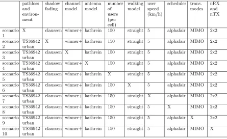
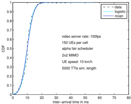
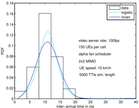
Figures 3 and 4 show the cumulative distribution function and the probability density function of the video streaming inter-arrival times, i.e., the time between the reception of two consecutive frames where the arriving time of a frame is the arriving time of the last packet of this frame. The inter-arrival time is called the jitter which is an important metric of the quality of service (QoS). A large jitter involves a bad QoS. For the video streaming applications, the media player has a deterministic rate which is the number of frames displayed per second (fps). There exist three main frame rate standards, 24 fps, 25 fps and 30 fps. For a rate of 25 fps, a frame is displayed every 40 ms. We can see on figure 4 that most of the inter-arrival times lay in the interval 10ms−20ms. This scenario corresponds to 150 users within a cell of diameter 500m.

These results confirm not only the performances of the LTE technology but also their importance for network provision-ing, predicting utilization of network resources, and for plan-ning network developments.

The fitting distributions are also an important result because we need to use theoretical models for research purpose. Of-ten it is difficult to work directly with the traffic traces of the content providers because they are not always accessible for confidentiality purpose; or simply because it is not practical. Then we develop mathematical models based on traditional queuing theory to compute streaming relative metrics such as the quality of service and the quality of experience.

0 10 20 30 40 50 60 70 80 0

0.1 0.2 0.3 0.4 0.5 0.6 0.7 0.8 0.9 1

inter−arrival time in ms

CDF

video server rate: 100fps 150 UEs per cell alpha fair scheduler 2x2 MIMO UE speed: 10 km/h 5000 TTIs sim. length

data logistic rician

(7)

0 5 10 15 20 25 30 35 40 0

0.02 0.04 0.06 0.08 0.1 0.12 0.14 0.16 0.18

inter−arrival time in ms

PDF

video server rate: 100fps

150 UEs per cell

alpha fair scheduler

2x2 MIMO

UE speed: 10 km/h

5000 TTIs sim. length data logistic rician

Figure 4: Probability density function of the inter-arrival times

Figure 5 shows the inter-arrival times autocorrelation

func-0 5 10 15 20

−0.5 0 0.5 1

Lag

Sample Autocorrelation

Sample Autocorrelation Function

Figure 5: Interarrival times autocorrelation function

tion. It computes the autocorrelation coefficients and plots them as a function of the lag. If the data are independent (uncorrelated) then the correlations should be near zero for all lags. We can see in the figure that the coefficients are not close to zero for many lags, that exhibit the long range dependence of the video streaming inter-arrival times.

6. CONCLUSIONS

In this paper, we consider the video streaming applications over the Long Term Evolution (LTE) networks. Our pur-pose is to analyze the video traffic data through the dynam-ics of the LTE networks. We use the Vienna LTE System Level Simulator for our study. Simulations were running with different values for the parameters: the pathloss, the users speed, the network layout, the transmission modes.

The video server was integrated to the simulator. Other types of traffic were also present. We process the simulation traces: For this purpose we consider the inter-arrival times of the streaming users because they are very important in the multimedia applications. They give an idea about the performances of the network. The best representation of the data is their distributions, i.e., the probability distribu-tion funcdistribu-tion and the cumulative distribudistribu-tion funcdistribu-tion. We use statistical methods like Maximum Likelihood Estimation and the Kalmogorov Smirnov test to fit the traffic data. We plot the PDF, the CDF and the fitting distributions using some functions of the statistical toolbox of MATLAB. We also plot the autocorrelation function which shows the long range dependance of the inter-arrival times.

From the plots, we can see that most of the inter-arrival times are in the interval 10ms-20ms. Knowing that the mean service time of the video playbacks is 40ms, that con-firms the high performance of the LTE networks.

Our results can be used to analyse the quality of experience of the video streaming applications and the quality of service of the LTE networks.

As future works, we plan to do the same simulations with ns-3, in order to compare the performances of the two sim-ulators.

ACKNOWLEDGMENT

This work has been carried out in the framework of IDE-FIX project, funded by the ANR under the contract number ANR-13-INFR-0006.

7. REFERENCES

[1] Mario Montagud, Fernando Boronat, and Vicent Vidal. Simulation platform for video streaming evaluation. pages 397–401, sept. 2010.

[2] Doggen Jeroen and Van der Schueren Filip. Design and simulation of a h.264 avc video streaming model. March 2008.

[3] Ahmed Bilal and Arshad M. Junaid. Simulation and comparative analysis of video streaming over adsl & wimax network.

[4] Biswapratapsingh Sahoo. Performance comparison of packet scheduling algorithms for video traffic in LTE

cellular network.IJMNCT, 3, June 2013.

[5] Jiasi Chen, Rajesh Mahindra, Mohammad Amir

Khojastepour, Sampath Rangarajan, and Mung Chiang. A scheduling framework for adaptive video delivery over cellular networks. pages 389–400. ACM, 2013.

[6] Xiaolin Cheng and Prasant Mohapatra. Quality-optimized downlink scheduling for video streaming applications in lte

networks. InGLOBECOM, pages 1914–1919. IEEE, 2012.

[7] Moustafa M Nasralla, CTER Hewage, and Maria G Martini. Subjective and objective evaluation and packet loss modeling for 3d video transmission over lte networks.

InTelecommunications and Multimedia (TEMU),

International Conference on, pages 254–259. IEEE, 2014. [8] Abdurrahman Fouda and al. Real-time video streaming

over ns3-based emulated lte networksk.IJECCT, 4, May

2014.

[9] Yuedong Xu, Eitan Altman, Rachid El-Azouzi, Majed Haddad, Salah-Eddine Elayoubi, and Tania Jimenez. Analysis of Buffer Starvation With Application to

Objective QoE Optimization of Streaming Services.IEEE

(8)

[10] E. Dahlman, S. Parkvall, J. Skold, and P. Beming.3G Evolution: HSDPA and LTE for Mobile Broadband. Academic Press, 2th edition, 2007.

[11] J. Zyren and Dr. W. McCoy.Overview of the 3GPP Long

Term Evolution Physical Layer, July 2007. [12] http://www.unwiredinsight.com/2013/lte-mimo. [13]

https://www.nt.tuwien.ac.at/downloads/featured-downloads/.

[14] J. C. Ikuno, M. Wrulich, and M. Rupp. System level

simulation of Lte networks.IEEE VTC2010-Spring, May

2010.

[15] Y. Xu, E. Altman, R. El-Azouzi, S. Elayoubi, and M. Haddad. Qoe Analysis of Media Streaming in Wireless

Data Networks.Springer Berlin Heidelberg, 2:343–354, May

2012.

[16] http://www.ist-winner.org/phase 2 model.html.

[17] IEEE Working Group 802.20 Permanent Document.Traffic

Models for IEEE 802.20 MBWA System Simulations, July 2003.

[18] Bozidar Vujicic, Nikola Cackov, Svetlana Vujicic, and Ljiljana Trajkovic. Modeling and characterization of traffic

in public safety wireless networks. InIn Proc. of SPECTS,

pages 214–223, 2005.

Video Streaming Analysis in Vienna LTE System Level Simulator